Estimation of Leaf Area Index Using DEIMOS-1 Data: Application and Transferability of a Semi-Empirical Relationship between two Agricultural Areas

 , ,
, ,  and
and
Abstract
: This work evaluates different procedures for the application of a semi-empirical model to derive time-series of Leaf Area Index (LAI) maps in operation frameworks. For demonstration, multi-temporal observations of DEIMOS-1 satellite sensor data were used. The datasets were acquired during the 2012 growing season over two agricultural regions in Southern Italy and Eastern Austria (eight and five multi-temporal acquisitions, respectively). Contemporaneous field estimates of LAI (74 and 55 measurements, respectively) were collected using an indirect method (LAI-2000) over a range of LAI values and crop types. The atmospherically corrected reflectance in red and near-infrared spectral bands was used to calculate the Weighted Difference Vegetation Index (WDVI) and to establish a relationship between LAI and WDVI based on the CLAIR model. Bootstrapping approaches were used to validate the models and to calculate the Root Mean Square Error (RMSE) and the coefficient of determination (R2) between measured and predicted LAI, as well as corresponding confidence intervals. The most suitable approach, which at the same time had the minimum requirements for fieldwork, resulted in a RMSE of 0.407 and R2 of 0.88 for Italy and a RMSE of 0.86 and R2 of 0.64 for the Austrian test site. Considering this procedure, we also evaluated the transferability of the local CLAIR model parameters between the two test sites observing no significant decrease in estimation accuracies. Additionally, we investigated two other statistical methods to estimate LAI based on: (a) Support Vector Machine (SVM) and (b) Random Forest (RF) regressions. Though the accuracy was comparable to the CLAIR model for each test site, we observed severe limitations in the transferability of these statistical methods between test sites with an increase in RMSE up to 24.5% for RF and 38.9% for SVM.1. Introduction
In the recent years, the use of satellite sensor data has become more common in precision agriculture technologies [1], and various operational services are being developed within the Global Monitoring for Environment and Security (GMES) initiative [2]. In this context, the data users (i.e., farmers, large and small scale agri-businesses) are mostly interested in monitoring the spatial distribution of some crop characteristics over the growing season and time-series of satellite acquisitions at high spatial resolution are a major source of information.
A key vegetation parameter attracting most interest is the Leaf Area Index (LAI), defined as the total one-sided area of green leaf area per unit ground surface area [3]. LAI is used to derive agronomical indicators for various crop management purposes. For instance, LAI maps are used in agro-meteorological models to derive the crop water needs (an example of operative application is given in Irrisat) [4], to monitor the nitrogen status and to apply fertilizer with variable rates (e.g., FarmSat), as input in crop models to derive agronomical variables [5,6]. On a larger scale, LAI and other biophysical variables are used for example for yield predictions at administrative level [7–9]. A general overview of remote sensing contributions to agriculture is given in [10].
Two groups of techniques have been commonly applied for the estimation of the LAI from optical satellite sensor data using semi-empirical/statistical approaches (i.e., vegetation indices, VI) or physical based approaches of leaf-canopy radiative transfer model (RTM) inversion [11,12]. Most of the empirical or statistical equations, such as regressions between spectral reflectance, vegetation indices (VI) or shape indices (e.g., red edge) and field measurements [13–15], employ data in two or more wavebands, usually red and near-infrared [16,17]. VIs are often the only option for the retrieval of LAI with limited spectral information (such as in the case of DEIMOS-1 data with only three spectral bands).
A prerequisite for the quantitative analysis of time-series of satellite sensor data is to perform radiometric and atmospheric corrections [18], if possible using reliable instantaneous atmospheric measurements (such as aerosol optical thickness, water vapor content) and/or the spectral reflectance of known ground targets either derived from ground measurements (surface and/or atmospheric conditions) or from consolidated library data [19,20]. Several approaches have been proposed for performing atmospheric corrections. An operative procedure is based on the use of look-up-tables (LUT) with pre-calculated atmospheric RTM simulations for different satellite sensor types [20,21]. However, model assumptions and simplifications often lead to inaccuracies in the estimated top-of-canopy (TOC) reflectance measurements [22].
The inherent inaccuracy of TOC reflectance data can be accounted for by using image-specific calibration procedures to estimate LAI. A typical example is the use of soil line-based VIs in place of intrinsic VIs [23]: in this case the image-specific tuning of the soil line slope parameter can be used to increase the consistency in the analysis of atmospherically corrected products, especially for time-series datasets.
In this study, the application of image-specific calibration procedures to estimate LAI was tested. We used satellite time-series from DEIMOS-1 data, an operational satellite in the DMC constellation, acquiring radiance in three spectral bands (green, red and near-infrared) at 22 m spatial resolution. DEIMOS-1 satellite is equipped with a wide-image-swath sensor (630 km), providing a large coverage and overlap between scenes and therefore increasing the revisit time and the probability of capturing cloud-free images. Considering the available spectral resolution of the sensor, we selected a simple LAI retrieval approach based on a VI using the CLAIR model [24]. This approach has been tested using canopy reflectance model data [24], field-based reflectance measurements [25] and satellite data in a number of studies [4,26].
The main goal of this work was to evaluate different operational strategies to identify the parameters of the semi-empirical CLAIR model to estimate LAI. Within this main goal, we assessed the transferability of the model parameters between test sites. For comparison, two relatively novel statistical methods were also investigated using Random Forest (RF) and Support Vector Machine (SVM) regressions.
In addressing these issues, the study provides recommendations for deriving consistent time-series maps of LAI in operational frameworks at moderate (22 m) spatial resolution with limited spectral information. Other statistical LAI mapping approaches are presented in other papers of this special issue [27].
2. Materials and Methods
2.1. Overview
The described methodology provides an operational perspective to identify the parameters of the semi-empirical CLAIR model [24,28] for deriving consistent time-series LAI maps. A set of DEIMOS-1 satellite sensor data were acquired over two agricultural regions in Southern Italy and Eastern Austria during one growing season. Contemporaneous field estimates of LAI were collected for a number of fields and crops. Using this dataset, three operational procedures were tested (Table 1). First, we considered a test site specific application based on seasonal average (constant) values of the CLAIR model parameters, namely the soil line slope, the WDVI∞ (representing the asymptotically limiting value for the Weighted Difference Vegetation Index (WDVI) when LAI tends to infinity) and the α extinction and scattering coefficient. Secondly, we derived the model parameters for each satellite acquisition separately. Finally, we tested an intermediate solution based on an image-specific estimation of the parameters that can be extracted directly from the images (i.e., soil line slope and WDVI∞) and on a seasonal average (constant) value of the parameter that requires contemporaneous field measurements (i.e., the α coefficient). Additionally, we evaluated the transferability of local models between the two test sites. For comparison, two other statistical methods to estimate LAI were also investigated: Random Forest (RF) and Support Vector Machine (SVM) regressions.
2.2. Field Experimental Campaigns
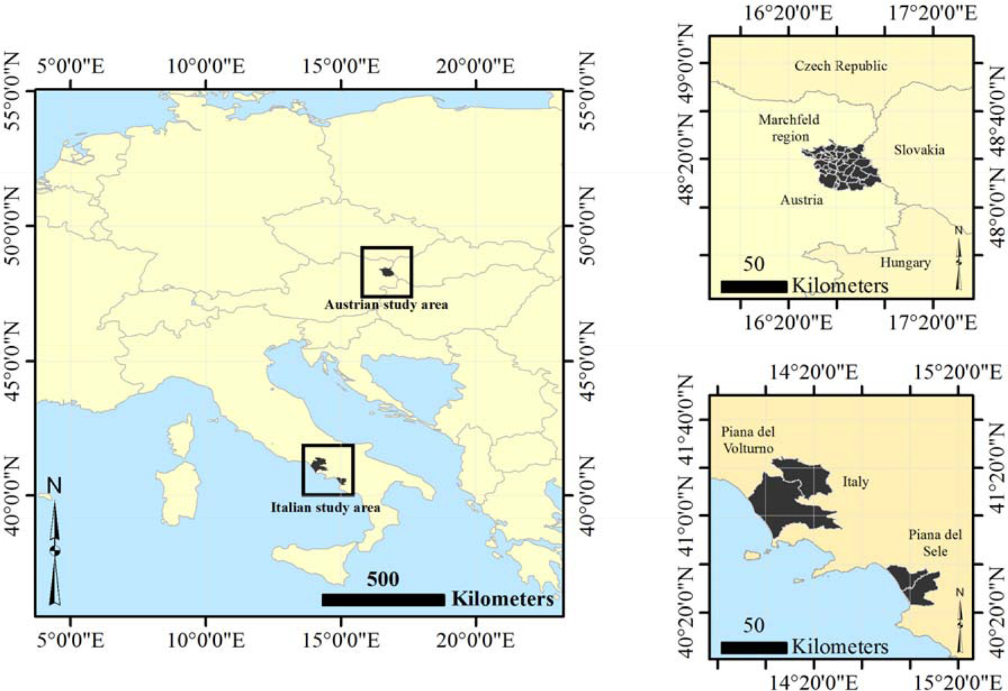
The field and satellite data used in this study were acquired in the context of two field campaigns carried out in two agricultural regions located in Southern Italy and in Eastern Austria during the 2012 growing season. The Italian field campaign was undertaken at the 500 km2 ‘Piana del Sele’ and at the 3820 km2 ‘Piana del Volturno’ sites in the Campania region of Southern Italy (Figure 1) (Lat. 40.52°N, Long. 15.00°E). The two sites are large agricultural regions and are characterized by irrigated agriculture (mainly forage crops, fruit trees and vegetables) with an average field size of about 2 ha [29]. The first site is characterized by very different soil types including Mollisols, Alfisols, Inceptisols and Entisols [30] according to the United States Department of Agriculture (USDA) soil taxonomy; the second plain is an alluvial formation with soil types varying from Entisols to Vertisols [31]. The average annual precipitation is about 800 mm, mostly concentrated during the winter months, with dry and warm summers. Maximum reference evapotranspiration rates, generally occurring during the second half of July, range between 3 and 5 mm/d [32].
The Austrian field campaign was undertaken at the 1000 km2 ‘Marchfeld region’ in Lower Austria (Lat. 48.20°N, Long. 16.72°E). The dominant soil types are Chernozem and Fluvisol, based on the Food and Agriculture Organization (FAO) World Soil Classification. The general soil conditions are characterized by a humus-rich A horizon and a sandy C horizon, followed by fluvial gravel from the former river bed of the Danube [33]. The region is characterized by a semi-arid climate with an average annual precipitation of 500–550 mm that can drop to 300 mm making it the driest region of Austria. Precipitation during the growing season (April–September) is 200–440 mm. Irrigation in Lower Austria has made it possible to establish a variety of crops thus contributing to the importance of Marchfeld in agricultural production. About 65000 ha of the area in Marchfeld are used for agricultural production. The main crops are vegetables (11%), sugarbeet (10%) and potatoes (7%).
Within these two large and relatively flat regions, LAI was estimated within 400 m2 elementary sampling units (ESU) that were relatively homogeneous in terms of both vegetation type and growth stage. The center of each ESU was geo-located by means of a GPS, with an accuracy of ±3–5 m.
For the Italian case study, LAI was sampled within ESUs over a period of three months (July–September 2012) in correspondence of each satellite acquisition for a total of 74 multi-temporal measurements comprising 11 ESUs (5 alfalfa and 6 maize fields in ‘Piana del Sele’) and 8 ESUs (3 alfalfa and 5 maize fields in ‘Piana del Volturno’). LAI values within the 19 ESUs ranged between 0.2 and 4.9 with a mean of 2.4 and a standard deviation of 1.2.
LAI in the ‘Marchfeld region’ was sampled within 55 ESUs for a range of crops including maize (10 ESUs), sugarbeet (7 ESUs), vineyards (7 ESUs), carrots (5 ESUs) and other crops (26 ESUs). LAI values within the 55 ESUs ranged between 0.1 and 5.8 with a mean of 2.2 and a standard deviation of 1.36. A summary of the field and satellite data acquisitions is given in Table 2.
LAI was estimated using the Plant Canopy Analyzer LAI-2000 [34]. Measurements were made during early morning and late afternoon under diffuse light conditions to minimize the effects of direct sunlight otherwise leading to LAI underestimation [35]. A view cap of 180 degrees was used to physically limit the sensor field-of-view and thus to reduce interference due to the presence of an operator. There are some limitations in this type of indirect measurements technique [36]. On the one hand, the LAI-2000 sensor does not distinguish photosynthetically active leaf tissue from other plant elements, such as stems, flowers or senescent leaves. This leads to overestimated LAI. On the other hand, the ‘clumping effect’, i.e., non-random positioning of canopy elements, is also neglected by the measurement device causing LAI underestimation. Hence, some compensation can be assumed [37]. The LAI recorded using the LAI-2000 sensor represents a measure close to the effective Plant Area Index (‘PAIe’) for reasons discussed above [37]. The average LAI, resulting from three replications of one above-canopy and nine below-canopy measurements, was taken as representative measure for each ESU. The three replications (for a total of 27 measurements) were sampled randomly within the ESU. The same sampling protocol was used in Austria and in Italy and throughout the three months field campaigns.
2.3. Satellite Data
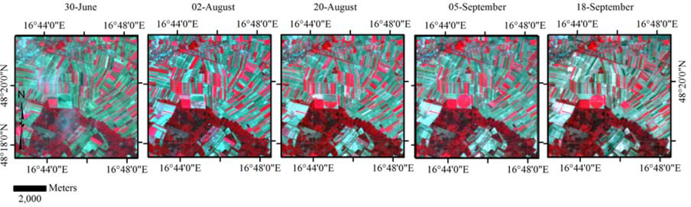
Multispectral data were acquired from DEIMOS-1, a satellite in the DMC constellation. The sensor records radiance in three broad spectral bands corresponding to green, red, and near-infrared parts of the electromagnetic spectrum at a ground sampling distance (GSD) of 22 m. Five and eight scenes were acquired during the 2012 growing season (Table 2) for the Austrian and for the Italian case studies, respectively. Satellite images were provided orthorectified to sub-pixel accuracy (∼10 m) using ground control points and the Shuttle Radar Topography Mission (SRTM v3) data as digital elevation model. The image data were atmospherically corrected by using ATCOR-2 [20]. For the Austrian test site, during the image acquisition campaign, five reference measurements of ground spectral reflectance (bare soils, dry and dense vegetation) were taken in correspondence of one satellite acquisition (August 2nd). A subset of these measurements was used to perform the atmospheric correction. The other subset was used to validate the results of the correction algorithm. The atmospheric correction for the other images in the time-series was cross-checked by observation of pseudo-invariant targets within the study area [19]. A similar procedure was used for the Italian test site and the accuracy of the atmospheric correction was checked against a set of reference pixels containing identifiable pseudo-invariant ground targets (i.e., asphalt, sea water, concrete and sand) with known reflectance values from a spectral library [20].
2.4. Estimation of Leaf Area Index
In this study, we selected a simple semi-empirical model and two statistical methods to estimate LAI. In all cases, we used the TOC (atmospherically corrected) reflectance data. Regarding the semi-empirical model, two spectral bands (red and near-infrared) were used to calculate the Weighted Difference Vegetation Index (WDVI), which was related to LAI through an inverse exponential relationship using the CLAIR model [24,28]. Regarding the statistical methods two models were applied: the first based on a regression tree algorithm using Random Forest (RF) and the second based on a linear kernel Support Vector Machine (SVM) regression.
2.4.1. Semi-Empirical Estimation of LAI with the CLAIR Model
The CLAIR model is based on an inverse exponential relationship between LAI and the WDVI, which was derived using field spectral radiometer data experimentally [24,28]. This relationship is built upon a simplified reflectance model of the light extinction through the vegetation canopy. The WDVI is calculated from the reflectance in red (ρred) and near-infrared (ρnir) as follows:
Different values of the parameters in Equation (2) can be found in the literature. For instance, Clevers [25] reported an α value ranging between 0.252 and 0.53 and WDVI∞ ranging between 68.6 and 57.9 for vegetative and generative growth stages of barley respectively.
In this study, we visually selected about 40–60 sample points of bare soils within each of the acquired satellite image data and the reflectance of these points was used for calculation of the soil line slope. The soil line slope was then used to calculate the WDVI. The WDVI∞ value was extracted for each image. Then, we derived the α coefficient using an unconstrained nonlinear optimization method, which minimizes the Root Mean Square Error (RMSE) (our cost function) between measurements and predictions of LAI values. An initial α value of 0.35 was used as first guess based on previous campaigns for the Italian test site. We checked different starting values, which always converged at the same final result.
We tested three different procedures (Table 1) to derive a set of α and WDVI∞ values to be applied throughout the growing season. Firstly we considered a test site specific estimation of the empirical parameters of Equations (1) and (2) obtaining one seasonal average (constant) value of the soil line slope and of WDVI∞. The α coefficient was derived using the pooled set of LAI measurements acquired during the three months campaign. In this way, the time-series field and satellite datasets were considered as a unique dataset. This procedure was repeated independently for each of the two test sites under investigation. In this case, we would perform field measurements for each new test site only during the first year or during short field campaigns before the operational activities. Once calibrated, the model parameters could be applied to the newly acquired images, without further need for field work.
The second procedure consisted in deriving a set of image-specific model parameters for each new satellite acquisition. In this case, we calibrated the α coefficient using only the LAI measurements acquired in correspondence of each acquisition. To avoid introducing biases related to measurements taken on different dates, we did not consider antecedent measurements. This procedure represents the most intensive and time consuming approach, in which we would need field campaigns for each new satellite overpass for the estimation of image-specific α coefficients. Similarly, we would extract a certain number of points from each image in order to calculate the soil line slope and the WDVI∞.
Differently, a constant α value to be applied throughout the growing season for each test site was considered as third procedure. This represents an intermediate solution in terms of resources required since we retain the same approach of the second case for deriving image-specific soil line slope and WDVI∞ values.
These three procedures reflect possible practical approaches for applying the CLAIR model in order to derive time-series of LAI maps in nearly real-time (48 h from satellite acquisitions) and for operational campaigns. For instance, the CLAIR model has been used to derive LAI for the calculation of crop water requirements in irrigation advisory services [4].
Considering the feasible size of the field datasets for this kind of analysis (74 and 55 measurements for Italy and Austria, respectively), the validation of the model performance was achieved by resampling the field dataset using a bootstrapping approach with 200 repetitions [39] in order to provide an unbiased estimation of the model accuracy [40]. To quantify the model prediction accuracies we used the following statistical measures: RMSE, the coefficient of determination (R2) between measured and predicted LAI and the confidence intervals.
2.4.2. Statistical Based Approaches for the Estimation of LAI: Support Vector Machine (SVM) and Random Forest (RF) Regression
A second group of techniques were applied for the estimation of LAI based on statistical models established using (1) a least-squares version of a support vector machine (SVM) regression and (2) a regression tree using Random Forest (RF) algorithm.
SVMs have been developed in the framework of statistical learning theory by Vapnik [41] for classification purposes and have been recently extended to regression problems [42]. SVMs have been applied for the estimation of LAI in previous studies [43–46] providing satisfactory results. A comprehensive tutorial for SVM regression was provided by [47]. In this study we used a SVM implemented by [48] as a Matlab toolbox. We selected a linear kernel function, which provided better results compared to polynomial or radial basis functions.
RF is an ensemble algorithm developed by Breiman [49]. It consists of several regression trees; each tree is trained on a bootstrap sample of the training dataset and the majority vote is taken for the RF prediction. Random subsets of input variables are used to train the regression tree. The algorithm provides an internal unbiased estimate of the error using the so-called ‘out-of-bag’ (OOB) samples. RF has been successfully used in several classification problems but limited application to biophysical vegetation parameters retrieval can be found in the literature [50,51]. In this study we used a Matlab implementation of RF [52] with a default set of model parameters (no. of trees = 500; no. of input variables randomly chosen at each split = 2).
For both SVM and RF, the regressions were established using LAI measurements and atmospherically corrected reflectance values in green, red and near-infrared bands. Additionally, date-specific WDVI and WDVI∞ values were used as input variables. This set of variables provided the most stable and accurate results compared to using seasonal average of WDVI and WDVI∞ values or reflectance only. In the case of SVM, we first optimized the regularization parameter γ of SVM model using a simplex search method and a leave-one-out cross validation approach with the experimental LAI dataset. Then, two models (one for each test site) were applied to the experimental datasets to calculate RMSE and R2. In the case of RF, the model performance was calculated using the RMSE obtained from the average OOB Mean Square Error (MSE) over 500 trees. A pseudo-coefficient of determination (pseudo-R2) was calculated as follows: 1 − MSE/variance (LAI).
3. Results and Discussion
3.1. Identification of the CLAIR Model Parameters and LAI Estimation Accuracy
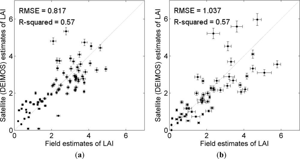
Procedure 1: the soil line slope and of the asymptotic limiting value for the WDVI (WDVI∞), along with the dates for field campaigns and satellite acquisitions are presented in Table 3. The α coefficient was derived using a bootstrap approach with 200 resampling of the experimental LAI dataset. The RMSE and R2 between measured and predicted LAI and the corresponding α coefficient were taken as the median values of the 200 bootstrap estimations. Prediction accuracies are presented in Table 4. The scatterplots between field and satellite estimates of LAI are shown in Figure 3. Applying this first procedure resulted in a RMSE of 0.817 and a R2 of 0.57 for the study region in Italy. For Austria, the RMSE was 1.037 and R2 was 0.57. It can be observed that the distance from the 1:1 line increases with higher values of both measured and estimated LAI. In addition, the variation of the actual estimates increases along with the LAI-value, an effect which was greatly reduced for the study region in Italy by using the second procedure. As expected, the RMSE for the Austrian case study was higher given the larger variability of the crop types in this area compared to Italy.
Procedure 2: the LAI measurements from the last two field campaigns (31/07 and 07/08, 13/08 and 10/09) and the corresponding image data for the Italian test site were combined in a single dataset due to a limited number of field measurements. Similarly, the LAI and image data from the last campaign (07/09 and 21/09) for the Austria test site were combined. The number of LAI measurements used for each image-specific calibration, including LAI statistics (minimum, maximum and mean values) is provided in Table 2.
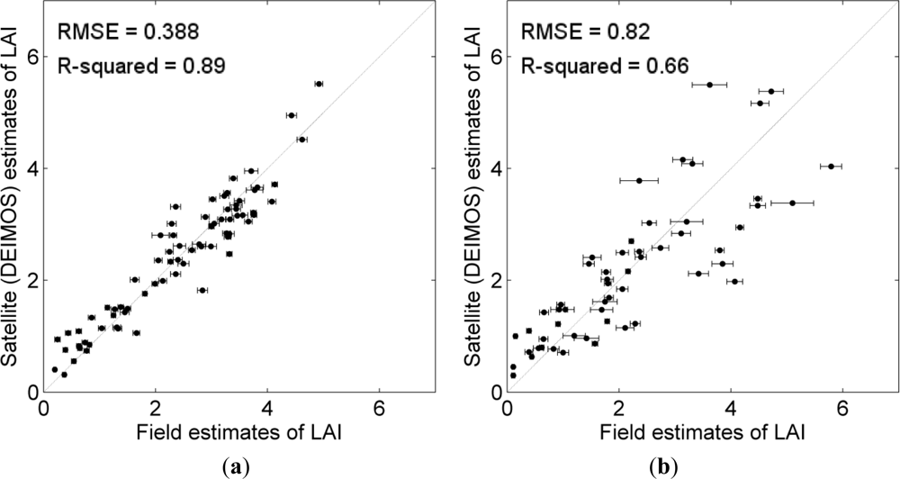
The scatterplots between field and satellite estimates of LAI are shown in Figure 4. Varying the soil line slope and thus WDVI values helped to improve WDVI based LAI estimation. Using the parameters (soil line slope and WDVI∞) listed in Table 3 resulted in an RMSE of 0.388 and R2 of 0.89 for the test site in Italy (Table 4). In addition, the higher variation of LAI estimation could be reduced when compared to the first procedure. For the Austrian test site the RMSE was 0.82 and R2 was 0.66. Analyzing the data presented in Table 4, we noticed that the range of variability of the α values (0.08) in the Austria test site is greater than the Italian one (0.04). This explains the larger RMSE observed in Austria as a consequence of the large crop variability in this area. In spite of this, larger errors are observed only for LAI values greater than 3.
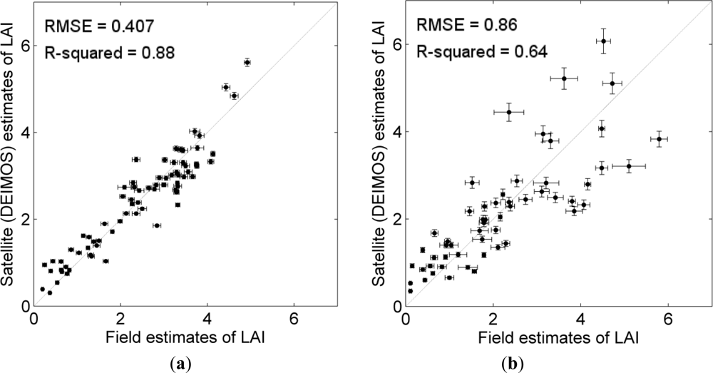
Procedure 3: results are presented in Table 4 and in Figure 5. A constant α coefficient value throughout the growing seasons and image-specific variation of soil line slope and WDVI∞ resulted in a RMSE of 0.407 and R2 of 0.88 for Italy and a RMSE of 0.86 and R2 of 0.64 for the Austrian test site. No substantial changes in the performance of the LAI estimation were observed when comparing this procedure to the full image-specific procedure. The slight increase in the RMSE is compensated by the reduced field work requirements of this approach.
3.2. Parameterization of Support Vector Machine and Random Forest (RF) Regressions and LAI Estimation Accuracy
The results of the SVM tuning provided a γ value of 0.5435 and 0.2998 for Italy and Austria, respectively. The application of tuned models (one for each test site) to the experimental datasets resulted in a RMSE of 0.394 and 0.785 for the Italian and for the Austria test sites, respectively. R2 resulted in 0.86 for Italy and 0.69 for Austria. The application of the RF regression achieved a RMSE (OOB) of 0.502 ± 0.027 and R2 of 0.82 for the Italian case study and a RMSE of 0.860 ± 0.017 and R2 of 0.63 for the Austrian case study. Compared to the CLAIR model performance, SVM achieved comparable accuracy for procedures 2 (Figure 4) and 3 (Figure 5) with image-specific soil line slope and WDVI∞ values. On the contrary, RF reported slightly lower accuracies for the Italian case study. However, the error estimates obtained from the OOB samples might be more realistic compared to the RMSE estimates for SVM.
3.3. Transferability of LAI Estimation Models from One Test Site to Another
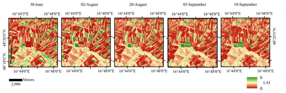
To test the transferability of the CLAIR model parameters from one test site to another we used the results obtained from the procedure 3 (see Table 1) based on image-specific soil line slope and WDVI∞, seasonal- and test site-specific α coefficients. An example of the LAI time-series maps derived with this procedure is presented in Figure 6.
The reciprocal exchange of the calibrated models resulted in a RMSE of 0.412 and R2 of 0.88 for the Italian test site. The RMSE for the Austrian test site was 0.855 with R2 of 0.64. Both datasets responded a slight LAI underestimation starting from measured LAI values of 2.3 and higher. Percentage variations in the RMSE compared to test site specific models were lower than 0.5%.
Similarly, we tested the transferability of the SVM and RF regressions between test sites. The application of RF models provided a RMSE of 0.747 when transferring to Italian case study and a RMSE of 0.906 for the Austrian case study. In this case, we observed poorer prediction power compared to test site specific models, with a percentage increase in the RMSE up to 24.5%.
The mutual application of the SVM regression models provided a RMSE of 0.783 and of 0.808 for the Italian and Austrian case study respectively, with a percentage increase of the RMSE up 38.9% compared to test site specific models. A summary of the results is provided in Table 5.
4. Conclusions
In this study, we described a methodology to derive consistent time-series of Leaf Area Index (LAI) maps using an exponential relationship (CLAIR model) between LAI and the soil-line based Weighted Difference Vegetation Index (WDVI). The study analyzed different procedures for estimating the CLAIR model parameters (soil line slope, WDVI∞ and α coefficient) and highlighted the operational aspects of these approaches. We tested a seasonal average (constant) and an image-specific tuning to increase the consistency in the analysis of atmospherically corrected time-series images. Additionally, we applied two other statistical methods based on Random Forest (RF) and Support Vector Machine (SVM) regressions. These two algorithms, applied in several remote sensing problems have proved particularly useful in recent years for land cover classification. However, few studies can be found in the remote sensing literature for their application to biophysical parameter prediction problems.
The experimental analysis was conducted using a set of DEIMOS-1 satellite sensor data acquired over two agricultural regions in Southern Italy and Eastern Austria. In particular, these data were acquired in the context of two satellite-based irrigation advisory services; LAI maps are used as input in agro-meteorological models to derive crop water needs. This information is delivered directly to the farmers for water management purposes in nearly real time. The Italian case study represents already an operational service, while the Austrian site is a test-bed for further development and testing transferability of models and procedures from different environments, agricultural and management practices. Although limited to one satellite type only, this dataset offered the possibility to evaluate the transferability of the model parameters from one test site to another. This is particularly relevant in case no field measurements are available.
Using the CLAIR model with an image-specific tuning of the soil line slope and WDVI∞ and a constant α coefficient value provided the most accurate and consistent results (RMSE = 0.407 and 0.86 for Italy and Austria respectively). Notably, this approach has the minimum requirements for fieldwork. Considering this procedure, we also evaluated the transferability of the local model parameters between the two test sites observing a decrease in estimation accuracies smaller than 0.5%. RF and SVM regressions provided comparable results for each test site. However, we observed severe limitations in the transferability of these statistical methods between test sites with an increase in RMSE up to 24.5% for RF and 38.9% for SVM.
This work indicates that the CLAIR model can provide satisfactory accuracy if an adequate model parameterization is performed; results achieved here (with a limited number of spectral inputs) do not justify the use of advanced regression techniques (such as RF and SVM) compared to simple and robust semi-empirical relationships. One advantage of the semi-empirical model used in this study is that its parameters have a physical denotation and it is possible to interpret and explain the model behavior. In addition, it has the advantage of not requiring a priori crop map information. This additional layer could be used, if available, to perform a crop specific calibration of the extinction and scattering coefficient (α). However, this would require additional fieldwork to achieve a statistically significant number of measurements for each crop type.
Acknowledgments
The study was supported by the Austrian Space Application Programme (ASAP) in the context of the project ‘EO4Water—Application of Earth observation technologies for rural water management’ ( www.eo4water.com) and by the ‘Irrigation Advisory Services’ of Campania Region, Italy ( www.irrisat.it).
References
- Lee, W.S.; Alchanatis, V.; Yang, C.; Hirafuji, M.; Moshou, D.; Li, C. Sensing technologies for precision specialty crop production. Comput. Electron. Agric 2010, 74, 2–33. [Google Scholar]
- NEREUS. The Growing Use of GMES across Europe’s Regions; NEREUS: Bruxelle, 2012. [Google Scholar]
- Bréda, N.J.J. Ground-based measurements of leaf area index: A review of methods, instruments and current controversies. J. Exp. Bot 2003, 54, 2403–2417. [Google Scholar]
- D’Urso, G.; Richter, K.; Calera, A.; Osann, M.A.; Escadafal, R.; Garatuza-Pajan, J.; Hanich, L.; Perdigão, A.; Tapia, J.B.; Vuolo, F. Earth Observation products for operational irrigation management in the context of the PLEIADeS project. Agric. Water Manage 2010, 98, 271–282. [Google Scholar]
- Jégo, G.; Pattey, E.; Liu, J. Using Leaf Area Index, retrieved from optical imagery, in the STICS crop model for predicting yield and biomass of field crops. Field Crops Res 2012, 131, 63–74. [Google Scholar]
- Casa, R.; Varella, H.; Buis, S.; Guérif, M.; De Solan, B.; Baret, F. Forcing a wheat crop model with LAI data to access agronomic variables: Evaluation of the impact of model and LAI uncertainties and comparison with an empirical approach. Eur. J. Agron 2012, 37, 1–10. [Google Scholar]
- Rembold, F.; Atzberger, C.; Rojas, O.; Savin, I. Using low resolution satellite imagey for yield prediction and yield anomaly detection. Remote Sens. 2013. under review.. [Google Scholar]
- Doraiswamy, P.C.; Sinclair, T.R.; Hollinger, S.; Akhmedov, B.; Stern, A.; Prueger, J. Application of MODIS derived parameters for regional crop yield assessment. Remote Sens. Environ 2005, 97, 192–202. [Google Scholar]
- Ma, G.; Huang, J.; Wu, W.; Fan, J.; Zou, J.; Wu, S. Assimilation of MODIS-LAI into the WOFOST model for forecasting regional winter wheat yield. Math. Comput. Model, 2011. in press.. [Google Scholar]
- Atzberger, C. Advances in remote sensing of agriculture: Context description, existing operational monitoring systems and major information needs. Remote Sens 2013, 5, 949–981. [Google Scholar]
- Baret, F.; Buis, S. Estimating Canopy Characteristics from Remote Sensing Observations: Review of Methods and Associated Problems. In Advances in Land Remote Sensing; Liang, S., Ed.; Springer: New York, NY, USA, 2008; pp. 173–201. [Google Scholar]
- Dorigo, W.A.; Zurita-Milla, R.; De Wit, A.J.W.; Brazile, J.; Singh, R.; Schaepman, M.E. A review on reflective remote sensing and data assimilation techniques for enhanced agroecosystem modeling. Int. J. Appl. Earth Obs. Geoinf 2007, 9, 165–193. [Google Scholar]
- Atzberger, C.; Guérif, M.; Baret, F.; Werner, W. Comparative analysis of three chemometric techniques for the spectroradiometric assessment of canopy chlorophyll content in winter wheat. Comput. Electron. Agric 2010, 73, 165–173. [Google Scholar]
- Cho, M.A.; Skidmore, A.K.; Atzberger, C. Towards red edge positions less sensitive to canopy biophysical parameters for leaf chlorophyll estimation using properties optique spectrales des feuilles (PROSPECT) and scattering by arbitrarily inclined leaves (SAILH) simulated data. Int. J. Remote Sens 2008, 29, 2241–2255. [Google Scholar]
- Darvishzadeh, R.; Atzberger, C.; Skidmore, A.K.; Abkar, A.A. Leaf Area Index derivation from hyperspectral vegetation indicesand the red edge position. Int. J. Remote Sens 2009, 30, 6199–6218. [Google Scholar]
- Chen, J.M.; Pavlic, G.; Brown, L.; Cihlar, J.; Leblanc, S.G.; White, H.P.; Hall, R.J.; Peddle, D.R.; King, D.J.; Trofymow, J.A.; et al. Derivation and validation of Canada-wide coarse-resolution leaf area index maps using high-resolution satellite imagery and ground measurements. Remote Sens. Environ 2002, 80, 165–184. [Google Scholar]
- Wang, Y.J.; Woodcock, C.E.; Buermann, W.; Stenberg, P.; Voipio, P.; Smolander, H.; Hame, T.; Tian, Y.H.; Hu, J.N.; Knyazikhin, Y.; Myneni, R.B. Evaluation of the MODIS LAI algorithm at a coniferous forest site in Finland. Remote Sens. Environ 2004, 91, 114–127. [Google Scholar]
- Liu, J.; Pattey, E.; Jégo, G. Assessment of vegetation indices for regional crop green LAI estimation from Landsat images over multiple growing seasons. Remote Sens. Environ 2012, 123, 347–358. [Google Scholar]
- Hadjimitsis, D.G.; Clayton, C.R.I.; Retalis, A. The use of selected pseudo-invariant targets for the application of atmospheric correction in multi-temporal studies using satellite remotely sensed imagery. Int. J. Appl. Earth Obs. Geoinf 2009, 11, 192–200. [Google Scholar]
- Richter, R. Correction of satellite imagery over mountainous terrain. Appl. Opt 1998, 37, 4004–4015. [Google Scholar]
- Liang, S.; Member, S.; Fang, H.; Chen, M. Atmospheric correction of Landsat ETM+ land surface imagery. I. Methods 2001, 39, 2490–2498. [Google Scholar]
- Laurent, V.C.E.; Verhoef, W.; Clevers, J.G.P.W.; Schaepman, M.E. Estimating forest variables from top-of-atmosphere radiance satellite measurements using coupled radiative transfer models. Remote Sens. Environ 2011, 115, 1043–1052. [Google Scholar]
- Baret, F.; Guyot, G. Potentials and limits of vegetation indices for LAI and APAR assessment. Remote Sens. Environ 1991, 35, 161–173. [Google Scholar]
- Clevers, J.G.P.W. Application of a weighted infrared-red vegetation index for estimating leaf Area Index by Correcting for Soil Moisture. Remote Sens. Environ 1989, 29, 25–37. [Google Scholar]
- Clevers, J.G.P.W.; Vonder, O.W.; Jongschaap, R.E.E.; Desprats, J.F.; King, C.; Prévot, L.; Bruguier, N. A semi-empirical approach for estimating plant parameters within the RESEDA-project. Int. Arch. Photogramm. Remote Sens. Spat. Inform. Sci. 2000, XXXIII, 272–279. [Google Scholar]
- Vuolo, F.; Atzberger, C.; Richter, K.; D’Urso, G.; Dash, J. Retrieval of Biophysical Vegetation Products from RapidEye Imagery. In ISPRS TC VII Symposium—100 Years ISPRS; Wagner, W., Szekely, B., Eds.; ISPRS: Vienna, Austria, 2010; Volume XXXVIII, pp. 281–286. [Google Scholar]
- Capodici, F.; D’Urso, G.; Maltese, A. Investigating the relationship between X-band SAR data from COSMOS-Skymed satellite and NDVI for LAI detection. Remote Sens. 2012. under review.. [Google Scholar]
- Clevers, J.G.P.W. The derivation of a simplified reflectance model for the estimation of leaf area index. Remote Sens. Environ 1988, 25, 53–69. [Google Scholar]
- De Michele, C.; Vuolo, F.; D’Urso, G.; Marotta, L.; Richter, K. The Irrigation Advisory Program of Campania Region: From research to operational support for the Water Directive in Agriculture. Proceedings of 33rd International Symposium on Remote Sensing of Environment (ISRSE), Stresa, Italy, 4–8 May 2009.
- Bonfante, A.; Alfieri, M.; Basile, A.; De Lorenzi, F.; Fiorentino, N.; Menenti, M. The Evaluation of the Climate Change Effects on Maize and Fennel Cultivation by Means of an Hydrological Physically Based Model: The Case Study of an Irrigated District. Proceedings of EGU General Assembly 2012, Vienna, Austria, 22–27 April 2012; p. 7807.
- Coppola, E.; Capra, G.F.; Odierna, P.; Vacca, S.; Buondonno, A. Lead distribution as related to pedological features of soils in the Volturno River low Basin (Campania, Italy). Geoderma 2010, 159, 342–349. [Google Scholar]
- Sequino, V.; Zucaro, R.; D’Alterio, D.; Valente, M.; Frunzio, M.; Iavarone, V.; Belmare, E.; Serpico, G. Stato dell’irrigazione in Campania, 1999, 109.
- Richter, K.; Rischbeck, P.; Eitzinger, J.; Schneider, W.; Suppan, F.; Weihs, P. Plant growth monitoring and potential drought risk assessment by means of Earth observation data. Int. J. Remote Sens 2008, 29, 4943–4960. [Google Scholar]
- LI-COR. LAI-2000 Plant Canopy Analyzer Instruction Manual Lincoln; LI-COR Inc.: Lincoln, NE, USA, 1992. [Google Scholar]
- Leblanc, S.G.; Chen, J.M. A practical scheme for correcting multiple scattering effects on optical LAI measurements. Agric. Forest Meteorol 2001, 110, 125–139. [Google Scholar]
- Welles, I.J.; Norman, J.M. Instrument for indirect measurement of canopy architecture. Agron. J 1991, 83, 818–825. [Google Scholar]
- Garriques, S.; Shabanov, N.V.; Swanson, K.; Morisette, J.T.; Baret, F.; Myneni, R.B. Intercomparison and sensitivity analysis of Leaf Area Index retrievals from LAI-2000, AccuPAR, and digital hemispherical photography over croplands. Agric. Forest Meteorol 2008, 148, 1193–1209. [Google Scholar]
- Baret, F.; Jacquemoud, S.; Hanocq, J.F. The soil line concept in remote sensing. Remote Sens. Rev 1993, 7, 65–82. [Google Scholar]
- Steyerberg, E.W.; Harrell, F.E.; Borsboom, G.J.; Eijkemans, M.J.; Vergouwe, Y.; Habbema, J.D. Internal validation of predictive models: Efficiency of some procedures for logistic regression analysis. J. Clin. Epidemiol 2001, 54, 774–81. [Google Scholar]
- Richter, K.; Atzberger, C.; Hank, T.B.; Mauser, W. Derivation of biophysical variables from Earth observation data: Validation and statistical measures. J. Appl. Remote Sens 2012, 6, 063557. [Google Scholar]
- Vapnik, V. The Nature of Statistical Learning Theory; Springer-Verlag: New York, NY, USA, 1995. [Google Scholar]
- Vapnik, V.; Golowich, S.E.; Smola, A.J. Support Vector Method for Function Approximation, Regression Estimation and Signal Processing. In Advances in Neural Information Processing Systems 9—Proceedings of the 1996 Neural Information Processing Systems Conference (NIPS 1996); Mozer, M., Jordan, M. I., Petsche, T., Eds.; MIT Press: Cambridge, MA, USA, 1997; pp. 281–287. [Google Scholar]
- Yang, X.; Huang, J.; Wu, Y.; Wang, J.; Wang, P.; Wang, X.; Huete, A.R. Estimating biophysical parameters of rice with remote sensing data using support vector machines. Sci. China. Life Sci 2011, 54, 272–81. [Google Scholar]
- Wang, F.; Huang, J.; Lou, Z. A comparison of three methods for estimating leaf area index of paddy rice from optimal hyperspectral bands. Precis. Agr 2011, 12, 439–447. [Google Scholar]
- Camps-Valls, G.; Munoz-Mari, J.; Gomez-Chova, L.; Richter, K.; Calpe-Maravilla, J. Biophysical parameter estimation with a semisupervised Support Vector Machine. IEEE Geosci. Remote Sens. Lett 2009, 6, 248–252. [Google Scholar]
- Verrelst, J.; Muñoz, J.; Alonso, L.; Delegido, J.; Rivera, J.P.; Camps-Valls, G.; Moreno, J. Machine learning regression algorithms for biophysical parameter retrieval: Opportunities for Sentinel-2 and -3. Remote Sens. Environ 2012, 118, 127–139. [Google Scholar]
- Smola, A.; Schölkopf, B. A tutorial on support vector regression. Statist. Comput 2004, 14, 199–222. [Google Scholar]
- Suykens, J.A.K.; Van Gestel, T.; De Brabanter, J.; De Moor, B.; Vandewalle, J. Least Squares Support Vector Machines; World Scientific Pub.Co.: Singapore, 2002. [Google Scholar]
- Breiman, L. Random Forests. Mach. Learn 2001, 45, 5–32. [Google Scholar]
- Powell, S.L.; Cohen, W.B.; Healey, S.P.; Kennedy, R.E.; Moisen, G.G.; Pierce, K.B.; Ohmann, J.L. Quantification of live aboveground forest biomass dynamics with Landsat time-series and field inventory data: A comparison of empirical modeling approaches. Remote Sens. Environ 2010, 114, 1053–1068. [Google Scholar]
- Le Maire, G.; Marsden, C.; Nouvellon, Y.; Grinand, C.; Hakamada, R.; Stape, J.-L.; Laclau, J.-P. MODIS NDVI time-series allow the monitoring of Eucalyptus plantation biomass. Remote Sens. Environ 2011, 115, 2613–2625. [Google Scholar]
- Liaw, A.; Wiener, M. Classification and regression by randomForest. R News 2002, 2, 18–22. [Google Scholar]


| Procedures | Soil Line Slope | WDVI∞ | α |
|---|---|---|---|
| 1 | constant | Constant | constant |
| 2 | image-specific | image-specific | image-specific |
| 3 | image-specific | image-specific | constant |
| Transferability | image-specific | image-specific | constant |
| Field Campaign Dates | Satellite Acquisition Dates | No. of Samples | LAI | ||
|---|---|---|---|---|---|
| Min | Max | Mean | |||
| Italy | (Sele // Volturno) | ||||
| 04/07 | 04/07 // 07/07 | 11 | 0.20 | 3.32 | 1.32 |
| 11/07 | 10/07 // 13/07 | 12 | 0.25 | 3.77 | 1.78 |
| 17/07 | 20/07 // 20/07 | 12 | 0.39 | 4.62 | 2.36 |
| 26/07 | 29/07 | 12 | 0.44 | 4.08 | 2.72 |
| 31/07 | 05/08 | 7 | 1.63 | 3.39 | 2.95 |
| 07/08 | 11/08 | 7 | 0.63 | 4.13 | 2.95 |
| 13/08 | 18/08 | 10 | 0.74 | 4.92 | 3.16 |
| 10/09 | 09/09 | 3 | 2.43 | 2.84 | 2.68 |
| Austria | (Marchfeld) | ||||
| 04/07 | 9 | 0.44 | 4.48 | 2.18 | |
| 02/08 | 20 | 0.11 | 4.52 | 1.75 | |
| 22/08 | Coincident with field campaigns | 10 | 0.15 | 3.31 | 1.82 |
| 07/09 | 6 | 1.79 | 5.79 | 2.83 | |
| 21/09 | 10 | 0.93 | 5.10 | 2.96 | |
| EO Acquisition Dates | Soil Line Slope | WDVI∞ | |
|---|---|---|---|
| Italy | (Sele // Volturno) | ||
| Seasonal average | 1.35 | 0.518 | |
| Seasonal Min-Max | 1.24–1.42 | 0.469–0.588 | |
| Image 1 | 04/07 // 07/07 | 1.37 // 1.33 | 0.493 // 0.488 |
| Image 2 | 10/07 // 13/07 | 1.38 // 1.32 | 0.50 // 0.495 |
| Image 3 | 20/07 // 20/07 | 1.37 // 1.42 | 0.469 // 0.538 |
| Image 4 | 29/07 | 1.33 // 1.37 | 0.56 |
| Image 5 | 05/08 | 1.33 // 1.38 | 0.485 |
| Image 6 | 11/08 | 1.24 / 1.38 | 0.588 |
| Image 7 | 18/08 | 1.30 // 1.38 | 0.48 // 0.525 |
| Image 8 | 09/09 | 1.31 | 0.54 |
| Austria | (Marchfeld) | ||
| Seasonal average | 1.47 | 0.596 | |
| Seasonal Min-Max | 1.41–1.64 | 0.57–0.61 | |
| Image 1 | 04/07 | 1.64 | 0.57 |
| Image 2 | 02/08 | 1.41 | 0.61 |
| Image 3 | 22/08 | 1.47 | 0.60 |
| Image 4 | 07/09 | 1.43 | 0.60 |
| Image 5 | 21/09 | 1.41 | 0.60 |
| Procedure | Case Study | Dataset | RMSE | R2 | α |
|---|---|---|---|---|---|
| 1 | Italy | Combined image 1–8 | 0.82 ± 0.01 | 0.58 | 0.32 ± 0.01 |
| Austria | Combined image 1–5 | 1.04 ± 0.03 | 0.58 | 0.39 ± 0.02 | |
| 2 | Italy | Image 1 | 0.23 ± 0.02 | 0.95 | 0.34 ± 0.02 |
| Image 2 | 0.24 ± 0.01 | 0.96 | 0.35 ± 0.01 | ||
| Image 3 | 0.24 ± 0.01 | 0.97 | 0.37 ± 0.01 | ||
| Image 4 | 0.49 ± 0.03 | 0.75 | 0.34 ± 0.02 | ||
| Image 5 & Image 6 | 0.44 ± 0.02 | 0.74 | 0.33 ± 0.01 | ||
| Image 7 & Image 8 | 0.54 ± 0.03 | 0.82 | 0.36 ± 0.02 | ||
| Austria | Image 1 | 0.79 ± 0.05 | 0.66 | 0.32 ± 0.03 | |
| Image 2 | 0.85 ± 0.03 | 0.64 | 0.40 ± 0.04 | ||
| Image 3 | 0.53 ± 0.04 | 0.78 | 0.32 ± 0.02 | ||
| Image 4 & Image 5 | 0.97 ± 0.04 | 0.54 | 0.32 ± 0.02 | ||
| 3 | Italy | Combined image 1–8 | 0.41 ± 0.004 | 0.88 | 0.35 ± 0.01 |
| Austria | Combined image 1–5 | 0.86 ± 0.01 | 0.64 | 0.34 ± 0.02 | |
| LAI Estimation Methods | Transferability | RMSE | R2 | Variations in RMSE (%) Compared to Test Site Specific Models |
|---|---|---|---|---|
| CLAIR model | IT with AT model | 0.412 | 0.88 | +0.2% |
| AT with IT model | 0.855 | 0.64 | −0.5% | |
| Random Forest | IT with AT model | 0.747 | 0.75 | +24.5% |
| AT with IT model | 0.906 | 0.61 | +4.6% | |
| Support Vector Machine | IT with AT model | 0.783 | 0.79 | +38.9% |
| AT with IT model | 0.808 | 0.69 | +2.3% |
Share and Cite
Vuolo, F.; Neugebauer, N.; Bolognesi, S.F.; Atzberger, C.; D'Urso, G. Estimation of Leaf Area Index Using DEIMOS-1 Data: Application and Transferability of a Semi-Empirical Relationship between two Agricultural Areas. Remote Sens. 2013, 5, 1274-1291. https://doi.org/10.3390/rs5031274
Vuolo F, Neugebauer N, Bolognesi SF, Atzberger C, D'Urso G. Estimation of Leaf Area Index Using DEIMOS-1 Data: Application and Transferability of a Semi-Empirical Relationship between two Agricultural Areas. Remote Sensing. 2013; 5(3):1274-1291. https://doi.org/10.3390/rs5031274
Chicago/Turabian StyleVuolo, Francesco, Nikolaus Neugebauer, Salvatore Falanga Bolognesi, Clement Atzberger, and Guido D'Urso. 2013. "Estimation of Leaf Area Index Using DEIMOS-1 Data: Application and Transferability of a Semi-Empirical Relationship between two Agricultural Areas" Remote Sensing 5, no. 3: 1274-1291. https://doi.org/10.3390/rs5031274