Mapping the Spatial Distribution of Winter Crops at Sub-Pixel Level Using AVHRR NDVI Time Series and Neural Nets


Abstract
: For large areas, it is difficult to assess the spatial distribution and inter-annual variation of crop acreages through field surveys. Such information, however, is of great value for governments, land managers, planning authorities, commodity traders and environmental scientists. Time series of coarse resolution imagery offer the advantage of global coverage at low costs, and are therefore suitable for large-scale crop type mapping. Due to their coarse spatial resolution, however, the problem of mixed pixels has to be addressed. Traditional hard classification approaches cannot be applied because of sub-pixel heterogeneity. We evaluate neural networks as a modeling tool for sub-pixel crop acreage estimation. The proposed methodology is based on the assumption that different cover type proportions within coarse pixels prompt changes in time profiles of remotely sensed vegetation indices like the Normalized Difference Vegetation Index (NDVI). Neural networks can learn the relation between temporal NDVI signatures and the sought crop acreage information. This learning step permits a non-linear unmixing of the temporal information provided by coarse resolution satellite sensors. For assessing the feasibility and accuracy of the approach, a study region in central Italy (Tuscany) was selected. The task consisted of mapping the spatial distribution of winter crops abundances within 1 km AVHRR pixels between 1988 and 2001. Reference crop acreage information for network training and validation was derived from high resolution Thematic Mapper/Enhanced Thematic Mapper (TM/ETM+) images and official agricultural statistics. Encouraging results were obtained demonstrating the potential of the proposed approach. For example, the spatial distribution of winter crop acreage at sub-pixel level was mapped with a cross-validated coefficient of determination of 0.8 with respect to the reference information from high resolution imagery. For the eight years for which reference information was available, the root mean squared error (RMSE) of winter crop acreage at sub-pixel level was 10%. When combined with current and future sensors, such as MODIS and Sentinel-3, the unmixing of AVHRR data can help in the building of an extended time series of crop distributions and cropping patterns dating back to the 80s.1. Introduction
Maps showing the spatial distribution of various crops are required for planning purposes, research and for assessing agricultural production [1,2]. Preferably, information regarding cropping patterns and intensities should also be made available for past decades, for assessing, for example, impacts of agricultural policies on land use. A plethora of possible uses of such information is reviewed in Atzberger [1]. Solutions for combining and homogenizing existing crop masks over large areas are illustrated in [3]. Historically, crop maps are generated by supervised classification of high resolution images. The images are generally acquired at key phenological stages for optimizing class separability. These approaches are labor and cost intensive, and require amounts of cloud-free high spatial resolution imagery. This impedes an operational implementation over large areas and in multiple years [4]. Data availability—particularly if specific crop stages need to be imaged—is often insufficient [5]. Additionally, these methods are usually affected by misclassification errors which can lead to strong bias in area estimates [6,7]. A good example of such approaches is described in Edlinger et al.[8], where the spatio-temporal development of irrigation systems in Uzbekistan is reconstructed from time series of Landsat imagery. Although generally feasible, the problems mentioned have limited the possibility of automatically updating land cover maps over large areas at regular (annual) intervals [9]. For example, for the US, it is expected that the Landsat-based National Land Cover Database (NLCD) will result in a six-year delay between data collection and product availability [10].
Low resolution images, on the other hand, are easily processed on a regional scale, and provide consistent information at high temporal frequency and cover large areas at low costs [11]. Additionally, low resolution data is available from the 1980s onward. Several current and planned missions such as MODIS, SPOT-VGT, Proba-V or Sentinel-3 ensure data continuity for the next 10–20 years. Classifications derived from such data can be updated at annual intervals as demonstrated by Lunetta et al. (2010) [12]. However, because of sub-pixel heterogeneity, the application of traditional hard classification approaches faces intrinsic methodological limitations and may result in significant errors in the estimated crop areas [9,13].
At the regional level, crop area estimations were significantly improved since the introduction of the MODIS sensor with 250 m ground resolution [9–15]. Not surprisingly, in these studies, the best results were obtained for agricultural areas such as the central plains of the United States and the Don River basin in Russia, where typical field sizes are large.
To address sub-pixel heterogeneity common for many areas of the world with fragmented landscapes, Quarmby et al. (1992) [16] used linear mixture model (LMM) techniques to coarse resolution data. Hansen et al. (2002) [17] used the continuous field algorithm for mapping vegetative traits, such as tree cover, using MODIS data. In the continuous field approach, each coarse resolution pixel is characterized as 0 to 100 percent cover of a vegetation class, ameliorating the primary limitation of coarse spatial resolution data [9].
Several authors combined high resolution images with NOAA AVHRR 1-km imagery to improve sub-pixel crop monitoring capabilities [18,19]. However, insufficient contrast between endmembers often leads to unstable solutions, resulting in inaccurate fraction images [4]. On the other hand, too few endmembers will fail to correctly represent the input signature.
A probabilistic linear unmixing approach with MODIS spectral/temporal data was developed and tested by Lobell and Asner (2004) [4]. The approach estimates sub-pixel fractions of crop area based on the temporal reflectance signatures throughout the growing season. In this approach, endmember sets are constructed using Landsat data to identify pure pixels, mainly located within large fields. Rather than defining endmembers with a single spectrum, endmembers are defined as a set of spectra which represent the full range of potential variability. The uncertainty in endmember fractions arising from endmember variability can then be quantified using Monte Carlo techniques. The performance of the proposed approach was assessed over Mexico and the Southern Great Plains and varied depending on the scale of comparison. Coefficients of determination ranged from greater 80% for crop cover within areas over 10 km2 to roughly 50% for estimating crop area within individual MODIS pixels.
Several studies by Rembold and Maselli used Spectral Angular Mapping (SAM) for measuring inter-annual crop area changes based on NDVI time series from NOAA-AVHRR [20,21]. The studies found that it was feasible to derive relatively accurate inter-annual winter crop acreage changes for the region of Tuscany, Italy. However, good results could be obtained only by estimating the crop acreage changes of single years from the average of a high number (7) of reference years. The results were significantly worse by using less or single years of reference data.
Regression tree analysis was used by Chang et al. (2007) [9] for the percentage of the corn and soybean area mapping using 500-m MODIS time series dataset. The strength of the regression tree is its use as a data mining tool. Numerous phenological measures and data transformations may be input to such a model to identify which ones are the most useful for crop-type discrimination.
Neural networks (NN) are powerful modeling tools, as they can learn and represent any kind of (non-linear) relationship between (a set of) input variables and (one or several) output variables, provided that enough nodes are used in the so-called hidden layer [22,23]. Lunetta et al. (2010) [12] used MODIS 16-day composite data to develop annual cropland and crop-specific map products for the Laurentian Great Lakes Basin. For the categorization of cropland and crop types, a multi-layer neural network classifier was used. Training pixels were identified using visual interpretation of MODIS-NDVI temporal profiles. The research included the application of an automated protocol to first filter the NDVI data to remove poor (corrupted) data values and then estimate the missing data using a discrete Fourier transformation technique. Atkinson et al. (1997) [22] showed how NN can be used for unmixing single date (5 wavebands) AVHRR imagery to map sub-pixel proportional land cover. The use of neural nets for estimating sub-pixel land cover from temporal signatures was investigated by Karkee et al. (2009) [24]. Braswell et al. (2003) [25] demonstrated that network based non-linear regression offers significant improvement relative to linear unmixing for estimation of sub-pixel land cover fractions in the heterogeneous disturbed areas of Brazilian Amazonia. The improvement was related to the fact that linear unmixing assumes the existence of pure sub-pixel classes (endmembers) with fixed reflectance signatures. The neural network approach proposed by Braswell et al. (2003) [25] estimates non-linear relationships between each land cover fraction and spectral-directional reflectances, without making assumptions about the physics of sub-pixel mixing.
In Verbeiren et al. (2008) [26] monthly standard maximum value compositing (MVC) of SPOT-VGT (between March and October) were used in neural nets to model the area fraction images (AFI) of eight classes in 2003 for Belgium. Relatively good results were obtained, especially if the initial (pixel-based) results were aggregated to coarser regional levels. The portability across growing seasons was investigated by Bossyns et al. (2007) [27] in an accompanying paper on the same dataset. The NNs were trained on data of one growing season and then applied to SPOT-VGT of the training year plus three additional seasons. High and stable accuracies of the estimated AFI’s were obtained for the training data. For example, at regional level, the R2 for winter wheat of the training years was ∼0.8 (0.67–0.87). On average, however, this value decreased by 0.45 units when the networks were applied to different seasons, probably because of a too high inter-annual variability of the endmembers.
To better cope with the natural year-to-year variability of NDVI profiles of vegetated surfaces, Atzberger and Rembold (2009) [28] trained networks with AVHRR time series. The target variable represented the sub-pixel winter crop fractional coverage. To permit the net distinguishing for various proportions of non-arable land within the mixed pixels (e.g., forested areas, urban land, etc.), available CORINE land cover information was used as additional input. A positive impact was demonstrated regarding the concurrent use of ancillary information and the applied temporal smoothing algorithm. In-season predictions improved compared to the work of Rembold and Maselli [20,21] using the same dataset and linear prediction models. The current paper is an extension and refinement of the mentioned paper. The main objective of the research is to test if neural networks can be fed with low resolution AVHRR imagery and additional ancillary information (derived from CORINE land cover) to estimate the spatio-temporal distribution of sub-pixel fractional winter crop coverages. The research is based on a multi-annual leave-one-out (bootstrapping) approach evaluated over an eight-year dataset acquired between 1988 and 2001. For this time period, reference information is available.
2. Material
The methodology was tested over the Tuscany region in Central Italy. The choice was driven mainly by the availability of satellite imagery and accurate agricultural statistics. The region is covered by a consistent NOAA-AVHRR data time series taken in the period from 1986 to 2001. For this period, eight Landsat scenes (TM/ETM+) are available in the study area, which can be used for the retrieval of reference data. An area frame sampling method [29] has been regularly applied since 1988 to measure the extent of the main crops in Tuscany. The selected test area is also interesting because of its challenging environmental setting with relatively small field sizes and changing cropping patterns.
2.1. Geography and Environmental Features of the Study Area
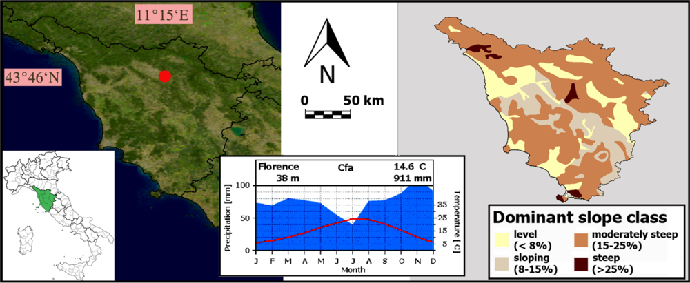
Tuscany is situated between 9°–12° East longitude and 44°–42° North latitude, covering circa 2 × 10⁶ ha (Figure 1). From an environmental point of view, Tuscany is peculiar for its extremely heterogeneous morphological and climatic features. The topography ranges from flat areas near the coastline and along the principal river valleys to hilly and mountainous zones towards the Apennine chain. Approximately two-thirds of the region is covered by hilly areas, one-fifth by mountains and only one-tenth by plains and valleys (Figure 1(right)). From a climatic viewpoint, Tuscany is influenced by its complex orographic structure and by the direction of the prevalent air flows (from West/Northwest). As a result, the climate ranges from typically Mediterranean to temperate warm or cool according to the altitudinal and latitudinal gradients and the distance from the sea. The average climatic conditions for the city of Florence are depicted in Figure 1(center).
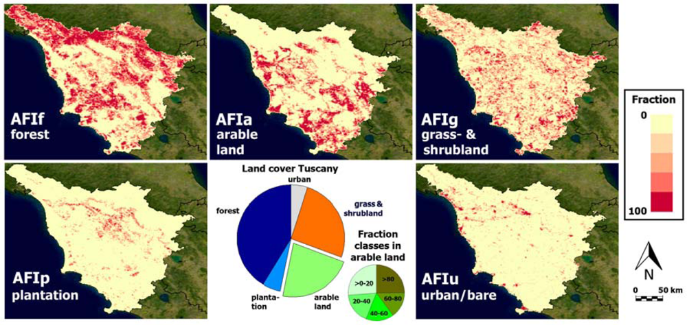
The land use of Tuscany is predominantly agricultural where the land is relatively flat (slope < 15%) (Figure 2) and where soil organic carbon content is high. In hilly and mountainous areas, mixed agricultural and forestry dominate. The main agricultural cover types are cereal crops in the plains and olive groves and vineyards on the hills. The upper mountain zones are almost completely covered by pastures and forests. Cropland is spread over the coastal zones, the inner plain and gently sloping hilly areas, covering approximately 20% of the land surface (Figure 2). The prevalent cereal is durum wheat, with an average planted area of 110,000 ha and with a mean growing cycle from November to the end of June (Figure 3). In areas with low percentage of arable land, forests and plantations occupy the main remaining area. When arable land dominates, the remaining area is mainly occupied by grass- and shrubland, in addition to urban land. Tuscany’s land cover and land use association is further detailed in Table 1.
2.2. Data
2.2.1. Reference Information on Winter Crop Areas
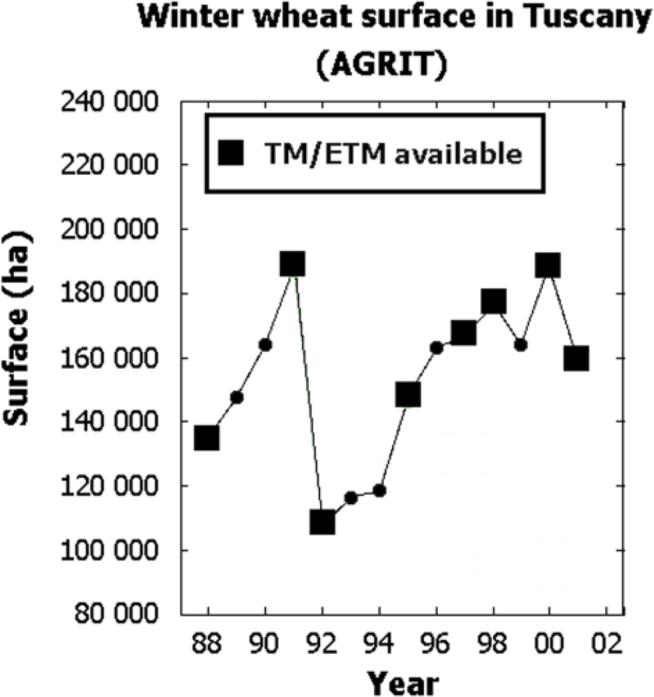
Wheat area estimates of Tuscany for the period 1988–2001 were obtained from the AGRIT project [30,31]. These statistics are produced annually through an area frame sampling method, which guarantees high estimation accuracy at the regional scale. At the regional level, the error for the main crops is generally lower than 10% [31]. In what follows, we use the term “winter crop area” as a synonym for the wheat area. The term “summer crop” designs the remaining crop land within the CORINE class “arable land.” Figure 4 displays the AGRIT winter crop area for the region of Tuscany between 1988 and 2001. A considerable variability can be seen, mainly as a direct result of European agricultural policies, market prices and weather conditions.
The land cover classification of Tuscany produced by the CORINE project was used (i) for deriving high resolution reference maps showing the spatial distribution of winter crops and (ii) as secondary input for the neural net. The Tuscan Regional Service for Cartography provided the necessary data. Data came in the form of a digitized map with a nominal scale of 1:100,000. The methodologies used for the production of the map, as well as its main features, are described by Annoni and Perdigao [5].
2.2.2. High Resolution Images
High resolution images were used for spatializing and disaggregating the statistical information provided by the AGRIT statistics. The high resolution dataset consisted of eight Landsat frames (192/30), six taken by the Thematic Mapper (TM) (1988, 1991, 1992, 1995, 1997 and 1998) and two by the Enhanced Thematic Mapper (ETM+) (2000, 2001). All of them were acquired during the month of August and were cloud free over the main agricultural areas.
The Landsat TM/ETM+ scenes were first georeferenced by a nearest neighbor resampling algorithm using about 120 control points selected on a land/water mask derived from the CORINE map. TM Bands 4 (nIR) and 3 (Red) were corrected for atmospheric effects and converted into reflectance images following the method proposed by Gilabert et al. (1994) [32]. The reflectances of these two bands were used to compute a high resolution NDVI image for every training year. The years for which Landsat TM/ETM+ imagery was available are highlighted in Figure 4 (large squares).
2.2.3. Low Resolution Images
The Joint Research Centre (JRC-MARS) of the European Commission owns the most elaborate archive of NOAA-AVHRR 1km data over the pan-European continent. The raw data were first collected by JRC itself, and since 2001, by VITO (Belgium). In 2008, all historical data were reprocessed with new procedures, which resulted in an unique archive of 29 years as described in Weiss et al. (2010) [33]. For this study, the AVHRR time series from 1988 to 2001 was used. The only recently updated NOAA AVHRR calibration coefficients [34] were not used.
3. Methods
3.1. Smoothing of Low Resolution AVHRR Data
Time series from AVHRR and other low to medium resolution sensors require a careful filtering/smoothing before they can be applied within quantitative studies [10]. The standard maximum value compositing (MVC) only corrects for major disturbances. To filter such data, a number of smoothing techniques are available [35,36]. For the current study, the Whittaker filter was chosen [37]. The Whittaker smoother is very fast and easy to parameterize, as it gives continuous control over smoothness with only one parameter. It also handles easily (large stretches of) missing values. In a recent comparative analysis of Atkinson et al. (2012) [38] the filter compared well with competing approaches, including Fast Fourier Transform (FFT), double logistics and asymmetric Gaussian functions.
Since the noise in the NDVI time series is negatively biased, a modified version of the original Whittaker smoother was used for this study [39,40]. Negatively biased noise results for example from undetected (sub-pixel) clouds and poor atmospheric conditions, depressing the observed NDVI values. The modifications ensured that the smoothed curves approach the upper envelope of the data. Similar techniques were suggested, for example, by Beck et al. (2006) [36] amongst others.
For providing crop acreage information not later than September–October of the current year, the filtered AVHRR data dekads 7–13 and 17–25 were extracted as inputs to the neural net (highlighted in Figure 3). During dekads 14–16, winter and “summer” crop signatures strongly overlap. These dekads were therefore excluded from the modeling. Only this reduced subset was used in the study.
3.2. Use of CORINE Data and Generation of Reference Abundance Maps Using Landsat Imagery
In the proposed approach, CORINE data was used twofold: (1) as network input (in addition to the AVHRR NDVI time series), and (2) for the generation of reference data. Using general land cover information as input (e.g., primary cover types), we take into account that (spatial) variations in the abundance of non-agricultural classes influence the observed temporal signature of two pixels, even if their respective winter/summer crop acreage is identical. The generation of reference data with high spatial resolution (e.g., abundance maps of winter crop acreages; AFIw) is necessary to validate the proposed methodology, as well as for network training (Figure 5).
For using CORINE data as network input, the 42 CORINE land cover classes were grouped into five environmentally meaningful categories with more or less similar NDVI profiles [5]. In addition to the “arable land” class, the following four primary cover types were derived: “forests,” “pastures,” “tree plantations” and “urban areas” [41] (Figure 2). For the study, we assumed that these five primary classes remain stable over the time period covered by the low resolution dataset (1988–2001). In addition, within each coarse resolution pixel, the sum of these five classes sum up to unity.
The fractional coverage of winter crops within the coarse resolution AVHRR grid was generated using available TM/ETM+ images from eight years (1988, 1991, 1992, 1995, 1997, 1998, 2000 and 2001) and splitting/disaggregating the CORINE “arable land” class into “winter crops” and remaining (“summer”) crops. To achieve this splitting, a simple NDVI thresholding approach was applied to each individual TM/ETM+ image. The rationale for this operation was that winter crop fields are almost bare in August, while other fields with summer crops (maize, sunflower, etc.) but also fallows and pastoral areas are in a “green” phase (Figure 3). Hence, any bare soil in August belongs to the class “winter crop.” The class “summer crop,” on the other hand is a mixture of typical summer crops with other classes.
As outlined, a NDVI threshold was optimized for each high resolution TM/ETM+ image to find the most appropriate cutting point distinguishing between bare soils and vegetation. To derive the spatial distribution of winter crops within the CORINE class “arable land,” for each TM/ETM+ image, different NDVI thresholds were systematically evaluated (0.1 ≤ threshold ≤ 0.25). For each threshold, the resulting (total) winter crop acreage was compared with the official AGRIT statistics. The threshold minimizing the difference between the reference information and the calculated winter crop acreage was retained and used to derive the high resolution winter crop masks.
The six categories identified in the eight training dates (five CORINE categories plus “winter crops”) were spatially degraded by pixel averaging to produce abundance images (i.e., area fraction images) with the same spatial resolution as the AVHRR images (Figure 2). Out of these maps, only the winter crop abundance maps (AFIw) were different for each date, as the other (CORINE) categories were assumed to be stable over time. The inter-annual variability of the reference winter crop acreages is shown in Figure 6 for all AVHRR pixels with at least 2 percent arable land.
It has to be noted that the TM/ETM+ frame 192/30 does not cover the entire region of Tuscany. Some small areas in the northern part of the region are not covered by the frame. These areas were therefore removed from the analysis, which corresponded to masking out 3.3% of the “arable land” class. The resulting error was regarded insignificant for the current study.
3.3. Neural Networking
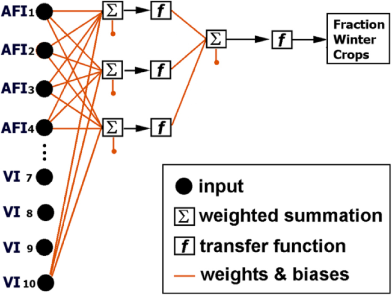
Network training consists in confronting a randomly initialized neural net of a given structure (topology) with training samples (= inputs + targets). In an iterative way, the values of weights and biases in the network are adjusted so as to minimize the error between the network output and the presented reference targets (here: winter crop abundances at pixel level). Once trained, even very large input datasets can be processed efficiently to produce the requested outputs [42,43].
For the present study, a simple NN with one hidden and one output layer was used (Figure 6). The output layer represented the winter crop fraction within a coarse resolution pixel and had thus only one node. Twenty-one input nodes were selected for modeling: 5 (inter-annually constant) abundance values derived from the CORINE data (e.g., arable land, forest, tree plantations, pasture and urban) (Figure 2), plus 16 nodes covering the NDVI profiles of the winter growing season (from dekad 7 to dekad 25), excluding the dekads 14–16 (Figure 3). The number of nodes in the hidden layer was set to 3, resulting in a compact 21-3-1 network architecture. Alternative architectures with a larger number of hidden nodes were evaluated [28] but resulted in overfitting problems.
For network training the resilient backpropagation algorithm was used within Matlab programming environment (The Mathworks Inc., Natick, MA, USA, 1994–2011). To achieve good generalization properties of the network, the early stopping technique described in Demuth and Beale (2003) [44] was applied. The training samples were split into three subsets with 50% (training), 25% (test) and 25% (validation) of the total available pattern. The training set was used for computing the gradient and updating the weights and biases. The error on the test set was monitored during the training process. When the network began overfitting the data, the test error started to rise. At this point, the training was stopped automatically and the actual weights at the minimum of the test error were returned. Nets trained in this way were subsequently used for estimating the target variable of the training and validation datasets.
For unbiased statistical results, a leave-one-out setting was chosen. For predicting the spatial distribution of winter crop fractional coverages, samples of seven out of eight years were used to train the net, which subsequently was applied to the left-out year, producing cross-validated results (Table 2). The cross-validated estimates of the sub-pixel winter crop abundances were then compared with the available TM/ETM+-derived reference information (each images each with 10,485 pixels containing arable land). Network portability across years was investigated in an accompanying paper [45] revealing good results.
4. Results
The (21-3-1) network was trained in a leave-one-out (jacknife) mode. Eight different nets were trained, each time using training vectors of seven out of the available eight years (Table 2). The left-out image was then predicted by the trained network. Statistics describing the accuracy of the spatialization of the predicted winter crop abundances for Tuscany are shown in Table 3 for each of the eight years of the dataset. To ease interpretation, the results are also summarized in Figure 7. The cross-validated statistics refer to the accuracy with which the (spatial distribution) of the abundance images has been modeled as compared to the Landsat TM/ETM+ -derived reference (AFIw) dataset. Figure 8 illustrates the findings for the year 2000 in form of a scatterplot between reference abundances and modeled results.
On average (median), 79 percent of the spatial variability of the (sub-pixel) winter crop abundances was explained by the network approach. The spatial distribution of winter crops was not equally well predicted across the eight years. The cross-validated coefficient of determination (R2cv) ranged between 0.70 (1988) and 0.82 (2000). The cross-validated RMSE values were around ∼10% (of winter crop area) and significantly higher than those obtained on the training samples (<9%) (not shown). Sometimes significant offsets were observed (see also large mean bias errors in Table 3).
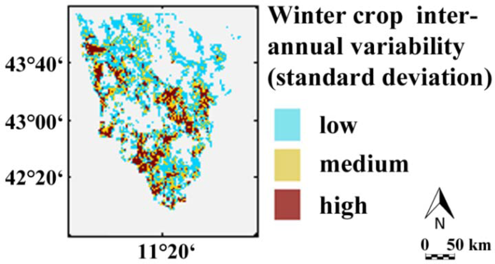
Maps of estimated winter crop abundances are shown in Figure 9 for the four most contrasting years of the eight-year dataset (cross-validated results). High winter crop acreages were reported for 1991 and 2000, whereas fewer winter crops were grown in 1988 and 1992 (Figure 4). This general tendency is well depicted by the estimates, as well as the general spatial distribution. The two maps at the top of Figure 9 report the inter-annual standard deviation (STD) of the winter crop area (AFIw) at the spatial resolution of NOAA-AVHRR. Again, it can be seen that the overall pattern is well represented by modeled maps, with albeit a significant underestimation of areas with high inter-annual variability (in red). This confirms the findings presented in Figure 8, where the regression line between reference information and estimated AFIw was < 1.
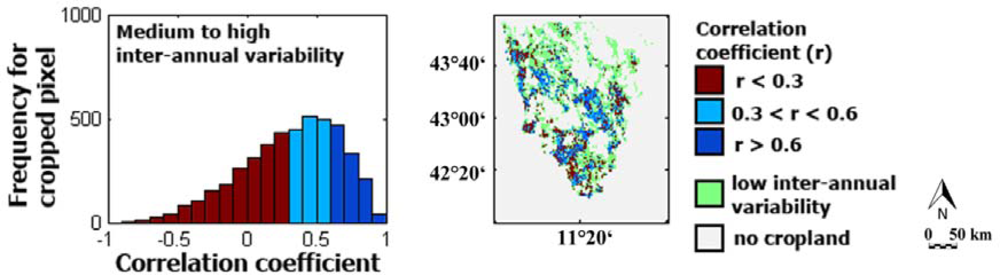
Results regarding the inter-annual variability of the retrieved sub-pixel estimates of AFIw are summarized in Figure 10. The map shows the multi-annual correlation coefficient between the reference winter crop fraction from high resolution imagery and the unmixing results. Only those AVHRR pixels are shown for which CORINE indicates arable land (≥2% arable land within the 1 km pixel) and where the inter-annual variability in the reference winter crop area (STD) was sufficiently high (≥5%). The corresponding frequency distribution is shown in the left panel. Inconsistent results appear. In some areas, the neural net performed acceptably well. However, low (or even negative) correlations were frequently obtained in the plains of Tuscany (indicated by red colors). In these areas, a high inter-annual variability of “summer crop” signatures can be observed. This variability prevented the net to correctly learn the relation between winter crop acreage and the NDVI temporal signature. In addition, quantitative interpretation of satellite data at pixel level is potentially confounded by errors in registration, as well as from adjacency effects [25]. Spatial averaging can minimize these problems, trading off resolution for overall accuracy. In this respect, the presented sub-pixel fractional cover estimates represent an extreme test case.
5. Discussion
The objective of this research was to evaluate the potential of simple neural networks for unmixing coarse resolution time series. For testing purposes, AVHRR NDVI data covering the time period between 1988 and 2001 at 1 km spatial resolution were unmixed for mapping the winter crop distribution in Tuscany, Italy. Encouraging results were obtained despite an environmentally complex and diverse study area, in addition to a limited amount of input data. An accompanying paper demonstrated the network portability across growing seasons [45]. The success relates partly to the compact network architecture selected for the study. Indeed, only three nodes were used in the hidden layer, albeit training samples could be predicted with higher accuracy if more complex networks were used [28]. The compact network guarantees robustness. In neural networking, overfitting and overspecialization problems increase with the number of nodes in the hidden layer. With only three nodes in the hidden layer—and receiving additional information regarding the fractional coverage of the five primary land cover classes (e.g., forest, plantation, urban, grassland and arable land)—a good compromise was found between network flexibility and robustness.
Past studies demonstrated the potential of using NDVI time series to study vegetation dynamics and (land cover) changes. The importance of image temporal frequency for accurately detecting forest changes was documented by Lunetta et al. (2004) [46]. The utility of NDVI time series is limited, however, by the availability of high-quality (e.g., cloud-free) data [10]. To cope with this critical factor, the AVHRR NDVI 1 km data used in the current study were pre-processed using a method developed by Eilers (2003) [37] and Atzberger and Eilers (2011) [39,40]. Pre-processing resulted in a filtered (anomalous data removed), cleaned (excluded and missing values estimated) and smoothed uninterrupted data stream supporting the neural networking. The quality of the selected smoother for filtering remotely sensed time series was confirmed in a recent study by Atkinson et al. (2012) [38], demonstrating that the smoother yields internally consistent data well representing the phenology of various vegetation cover types. In the conference paper of [28] using the same data as for the current study, a positive effect of the filtering was noted when compared to results using the original AVHRR data.
One problem which could not be solved relates to the class of “summer” crops. This broad class—defined as arable land which is not winter crop—can show a high inter-annual (and spatial) variability. This could be clearly seen both in the inner and coastal plains of Tuscany. In these areas, it is known that the proportion, composition and phenology of summer crops have a high inter-annual variability. Attempts were made to minimize the negative effects related to the mentioned variability of temporal “summer” crop signatures by excluding time stamps in the NDVI time series where winter and summer crops strongly overlap. Future research should focus on methods for deriving more detailed information regarding the different summer crops, instead of using one class merging quite different crops together.
Thus far, the utility of time series derived from radiometrically improved sensors such as MODIS or SPOT-VGT was not assessed. Possibly, some improvements could be made. Such improvements would come at the cost, however, of much shorter time series. Only by using data from NOAA AVHRR, would it be possible to globally monitor cropping patterns back to the eighties of the last century. The study demonstrated that it is possible to base such an analysis on internally consistent NDVI profiles from AVHRR starting in 1988 if a suitable filter is applied to smooth the data prior to data analysis. The use of a different low resolution input dataset would probably have resulted in different results. For example, Yin et al.[47] observed differences in satellite-derived NDVI trends over Inner Mongolia using SPOT-VGT and NOAA AVHRR datasets. In the study of Meroni and colleagues (2012) [48], it was demonstrated that vegetation products derived from the same sensor (SPOT-VGT) can differ, depending on the applied pre-processing. Such issues, however, were not part of the studied research questions.
Several studies pointed out that the primary limitation for crop-type mapping is not the input data or the employed unmixing algorithm, but the presence of high-quality training information for model calibration [9]. In this respect, it has to be mentioned that the current study did not evaluate the quality of the high resolution reference information derived from official AGRIT statistics and Landsat TM/ETM+ data. Implicitly, it was assumed that the spatialization of the regional (AGRIT) statistic—and the statistic itself—were accurate. If this assumption fails, the net will be trained and evaluated against erroneous data. To overcome this problem, it would be necessary to acquire some ground truth through field studies. This was beyond the scope of the present study.
6. Conclusions
The study evaluated the performance of neural networks for mapping the spatial distribution of winter crops using low resolution imagery and ancillary information. The strength of the neural net is its speed in processing large amounts of data and its capability to integrate remotely sensed time series and ancillary information derived from existing land cover maps. The selected backpropagation network was useful in deriving reasonable estimates of sub-pixel winter crop acreages from AVHRR time series. Sub-pixel winter crop acreages (0 to 100%) were estimated with cross-validated R2 of around 0.8 and RMSE of 10%. The results were improved compared to an earlier study using the same dataset but based on spectral angular mapping (SAM) of temporal NDVI profiles [21]. Although the performance of the neural nets decreased when applied to different growing seasons, the drop in accuracy was not as strong as found, for example, by Bossyns et al. (2007) [27].
We attribute the robustness of the proposed neural network approach to the fact that ancillary data has been used (together with NDVI time profiles) as inputs to the neural net. The use of ancillary information allows the net to better distinguish NDVI time series from pixels with similar proportions of winter crops and arable land but with different “background” contributions (e.g., various proportions of forests, pastures and plantations within the non-arable land). Other input datasets can then easily be adapted to operational settings. If possible, any known intra-class variability showing spatial patterns and multi-annual variations should be taken into account. For example, one could use available high resolution images to define spectral sub-classes within the pre-defined land cover classes. Future research should also evaluate the usefulness of additional network inputs, such as indicators of vegetation phenology, meteorological indicators, and/or DEM-derived indicators.
As for any other modeling tool, in neural networking, the quality of the provided reference information is of utmost importance. In the present study, reference information concerning the sub-pixel crop acreages was successfully derived from official regional statistics using a simple thresholding approach applied to high resolution Landsat TM/ETM+ imagery. In the optimum case, data from growing seasons covering the most “extreme” cropping pattern should be made available for network training. In the accompanying paper from the same authors studying the portability of neural nets across the growing season [45], it was demonstrated that three carefully chosen reference years are, in principle, sufficient for obtaining reasonable results. Using data from years with “extreme” cropping pattern avoids later confrontation of the network with input vectors not seen during the training step. Following the same logic, solutions have to be developed to minimize effects of shifts in vegetation phenology related, for example, to extreme weather conditions during the sowing period. If such effects are not minimized, the net will misinterpret shifting NDVI profiles as being the result of crop acreage changes.
Considering the results obtained, we intend on testing the approach in other landscapes (both important crop production areas and food-insecure countries) and to evaluate other low/medium resolution NDVI time series (e.g., MODIS). Main requirements in this sense are the availability of (1) training data for the discrimination between winter and summer crops, either based on high resolution data analysis or using existing agricultural databases (e.g., high resolution land use classifications or cadastral data) [26], and (2) reliable crop area statistics, possibly based on a high accuracy area frame sampling approach, such as the AGRIT project at the provincial or national level.
References
- Atzberger, C. Advances in remote sensing of agriculture: Context description, existing operational monitoring systems and major information needs. Remote Sens 2013, 5, 949–981. [Google Scholar]
- Rembold, F.; Atzberger, C.; Savin, I.; Rojas, O. Using low resolution imagery for yield prediction and yield anomaly detection. Remote Sens. 2013. in press. [Google Scholar]
- Vancutsem, C.; Marinho, E.; Kayitakire, S.L.; Fritz, S. Harmonizing and combining existing land cover/land use datasets for cropland area monitoring at the African. Remote Sens 2013, 5, 19–41. [Google Scholar]
- Lobell, D.B.; Asner, G.P. Cropland distributions from temporal unmixing of MODIS data. Remote Sens. Environ 2004, 93, 412–422. [Google Scholar]
- Annoni, A.; Perdigao, V. Technical and Methodological Guide for Updating CORINE Land Cover Data Base; EUR 17288EN; European Commission: Ispra, Italy, 1997. [Google Scholar]
- Czaplevsky, R.L. Misclassification bias in areal estimates. Photogram. Eng. Remote Sensing 1992, 58, 189–192. [Google Scholar]
- Gallego, F.J. Remote sensing and land cover area estimation. Int. J. Remote Sens 2004, 25, 3019–3047. [Google Scholar]
- Edlinger, J.; Conrad, C.; Lamers, J.; Khasankhanova, G.; Koellner, T. Reconstructing the spatio-temporal development of irrigated production systems in Uzbekistan using Landsat time series. Remote Sens 2012, 4, 3972–3994. [Google Scholar]
- Chang, J.; Hansen, M.C.; Pittman, K.; Carroll, M.; DiMiceli, C. Corn and soybean mapping in the United States using MODIS time-series data sets. Agron. J 2007, 99, 1654–1664. [Google Scholar]
- Lunetta, R.S.; Knight, J.F.; Ediriwickrema, J.; Lyon, J.G.; Worthy, L.D. Land-cover change detection using multi-temporal MODIS NDVI data. Remote Sens. Environ 2006, 105, 142–154. [Google Scholar]
- Vuolo, F.; Atzberger, C. Exploiting the classification performance of Support Vector Machines with multi-temporal moderate-resolution imaging spectroradiometer (MODIS) data in areas of agreement and disagreement of existing land cover products. Remote Sens 2012, 4, 3143–3167. [Google Scholar]
- Lunetta, R.S.; Shao, Y.; Ediriwickrema, J.; Lyon, J.G. Monitoring agricultural cropping patterns across the Laurentian Great Lakes Basin using MODIS-NDVI data. Int. J. Appl. Earth Obs. Geoinf 2010, 12, 81–88. [Google Scholar]
- Defries, R.S.; Field, C.B.; Fung, I.; Justice, C.O.; Los, S.; Matson, P.A.; Matthews, E.; Mooney, H.A.; Potter, C.S.; Prentice, K.; et al. Mapping the land-surface for global atmosphere-biosphere models—Toward continuous distributions of vegetations functional properties. J. Geophys. Res 1995, 100, 20867–20882. [Google Scholar]
- Wardlow, B.D.; Egbert, S. Large-area crop mapping using time-series MODIS 250 m NDVI data: An assessment for the U.S. Central Great Plains. Remote Sens. Environ 2008, 112, 1096–1116. [Google Scholar]
- Fritz, S.; Massart, M.; Savin, I.; Gallego, J.; Rembold, F. The use of MODIS data to derive acreage estimations for larger fields: A case study in the south-western Rostov region of Russia. Int. J. Appl. Earth Obs. Geoinf 2008, 10, 453–466. [Google Scholar]
- Quarmby, N.A. Linear mixture modelling applied to AVHRR data for crop area estimation. Int. J. Remote Sens 1992, 13, 415–425. [Google Scholar]
- Hansen, M.C.; DeFries, R.S.; Townshend, J.R.G.; Sohlberg, R.; Dimiceli, C.; Carroll, M. Towards an operational MODIS continuous field of percent tree cover algorithm: Examples using AVHRR and MODIS data. Remote Sens. Environ 2002, 83, 303–319. [Google Scholar]
- Maselli, F.; Gilabert, M.A.; Conese, C. Integration of high and low resolution NDVI data for monitoring vegetation in Mediterranean environments. Remote Sens. Environ 1998, 63, 208–218. [Google Scholar]
- Doraiswamy, P.C.; Hatfield, J.L.; Jackson, T.J.; Akhmedov, B.; Prueger, J.; Stern, A. Crop condition and yield simulations using Landsat and MODIS. Remote Sens. Environ 2004, 92, 548–559. [Google Scholar]
- Rembold, F.; Maselli, F. Estimating inter-annual crop area variation using multi-resolution satellite sensor images. Int. J. Remote Sens 2004, 25, 2641–2647. [Google Scholar]
- Rembold, F.; Maselli, F. Estimation of inter-annual crop area variation by the application of spectral angle mapping to low resolution multitemporal NDVI images. Photogram. Eng. Remote Sensing 2006, 72, 55–62. [Google Scholar]
- Atkinson, P.M.; Cutler, M.E.J.; Lewis, H. Mapping sub-pixel proportional land cover with AVHRR imagery. Int. J. Remote Sens 1997, 8, 917–935. [Google Scholar]
- Atkinson, P.M.; Tatnall, A.R.L. Neural networks in remote sensing. Int. J. Remote Sens 1997, 18, 699–709. [Google Scholar]
- Karkee, M.; Steward, B.L.; Tang, L.; Aziz, S.A. Quantifying sub-pixel signature of paddy rice field using an artificial neural network. Comput. Electron. Agric 2009, 65, 65–76. [Google Scholar]
- Braswell, B.H.; Hagen, S.C.; Frolking, S.E.; Salas, W.A. A multivariable approach for mapping sub-pixel land cover distributions using MISR and MODIS: Application in the Brazilian Amazon region. Remote Sens. Environ 2003, 87, 243–256. [Google Scholar]
- Verbeiren, S.; Eerens, H.; Picard, I.; Bauwens, I.; van Orshoven, J. Sub-pixel classification of SPOT-VEGETATION time series for the assessment of regional crop areas in Belgium. Int. J. Appl. Earth Obs. Geoinf 2008, 10, 486–497. [Google Scholar]
- Bossyns, B.; Eerens, H.; van Orshoven, J. Crop Area Assessment Using Sub-Pixel Classification with a Neural Network Trained for a Reference Year. Proceedings of the 4th International Workshop on the Analysis of Multi-Temporal Remote Sensing Imagery, Leuven, Belgium, 18–20 July 2007; pp. 1–8.
- Atzberger, C.; Rembold, F. Estimation of inter-annual winter crop area variation and spatial distribution with low resolution NDVI data by using neural networks trained on high resolution images. Proc. SPIE 2009. [Google Scholar] [CrossRef]
- Carfagna, E.; Ragni, P.; Balli, F. Crop Production Agricultural Survey Based on Area Frame Sampling Methods (1988–1997). In FAO Statistical Development Series; Gonzales-Villalobos, A., Wallace, A., Eds.; FAO: Rome, Italy, 1998; Chapter 13; pp. 203–216. [Google Scholar]
- AGRIT 2009. Cereali Autunno-Vernini Statistiche Agronomiche di Superficie, Resa e Produzione; Bollettino Giugno 2009; Sistema Informativo Nazionale per lo sviluppo in Agricoltura: Rome, Italy, 2009.
- Consorzio, I.T.A. Telerilevamento in Agricoltora, Previsione delle Produzioni di Frumento in Tempo Reale e Sviluppi Tecnologici; Ministero dell’Agricultura: Rome, Italy, 1987. [Google Scholar]
- Gilabert, M.A.; Conese, C.; Maselli, F. An atmospheric correction method for automatic retrieval of surface reflectances from TM images. Int. J. Remote Sens 1994, 15, 2065–2086. [Google Scholar]
- Weiss, M.; Baret, F.; Eerens, H.; Swinnen, E. FAPAR over Europe for the Past 29 Years: A Temporally Consistent Product Derived from AVHRR and VEGETATION Sensors. Proceedings of the 3rd International Symposium on Recent Advances in Quantitative Remote Sensing, Valencia, Spain, 27 September–1 October 2010; pp. 428–433.
- Molling, C.C.; Heidinger, A.K.; Staka, W.C., III; Wu, X. Calibrations for AVHRR Channels 1 and 2: Review and path towards consensus. Int. J. Remote Sens 2010, 31, 6519–6540. [Google Scholar]
- Chen, J.; Jönsson, P.; Tamura, M.; Gu, Z.; Matsushita, B.; Eklundh, L. A simple method for reconstructing a high-quality NDVI time-series data set based on the Savitzky–Golay filter. Remote Sens. Environ 2004, 91, 332–334. [Google Scholar]
- Beck, P.; Atzberger, C.; Høgda, K.; Johansen, B.; Skidmore, A. Improved monitoring of vegetation dynamics at very high latitudes: A new method using MODIS NDVI. Remote Sens. Environ 2006, 100, 321–334. [Google Scholar]
- Eilers, P.H.C. A perfect smoother. Anal. Chem 2003, 75, 3299–3304. [Google Scholar]
- Atkinson, P.M.; Jeganathan, C.; Dash, J.; Atzberger, C. Inter-comparison of four models for smoothing satellite sensor time-series data to estimate vegetation phenology. Remote Sens. Environ 2012, 123, 400–417. [Google Scholar]
- Atzberger, C.; Eilers, P.H.C. A time series for monitoring vegetation activity and phenology at 10-daily time steps covering large parts of South America. Int. J. Digit. Earth 2011, 4, 365–386. [Google Scholar]
- Atzberger, C.; Eilers, P.H.C. Evaluating the effectiveness of smoothing algorithms in the absence of ground reference measurements. Int. J. Remote Sens 2011, 32, 3689–3709. [Google Scholar]
- Maselli, F. Definition of spatially variable spectral endmembers by locally calibrated multivariate regression analysis. Remote Sens. Environ 2001, 75, 29–38. [Google Scholar]
- Mas, J.F.; Flores, J.J. The application of artificial neural networks to the analysis of remotely sensed data. Int. J. Remote Sens 2008, 29, 617–663. [Google Scholar]
- Foody, G.M.; Lucas, R.M.; Curran, P.H.; Honzak, M. Non-linear mixture modeling without end-members using an artificical neural net. Int. J. Remote Sens 1997, 18, 937–953. [Google Scholar]
- Demuth, H.; Beale, M. Neural Network Toolbox User’s Guide, Version 4; The MathWorks Inc: Natick, MA, USA, 2003. [Google Scholar]
- Atzberger, C.; Rembold, F. Portability of neural nets modelling regional winter crop acreages using AVHRR time series. Eur. J. Remote Sens 2012, 45, 371–392. [Google Scholar]
- Lunetta, R.S.; Johnson, D.M.; Lyon, J.G.; Crotwell, J. Impacts of imagery temporal frequency on land-cover change detection monitoring. Remote Sens. Environ 2004, 89, 444–454. [Google Scholar]
- Yin, H.; Udelhoven, T.; Fensholt, R.; Pflugmacher, D.; Hostert, P. How NDVI trends from AVHRR and SPOT VGT time series differ in agricultural areas: An Inner Mongolian case study. Remote Sens 2012, 4, 3364–3389. [Google Scholar]
- Meroni, M.; Atzberger, C.; Vancutsem, C.; Gobron, N.; Baret, F.; Lacaze, R.; Eerens, H.; Leo, O. Evaluation of agreement between space remote sensing SPOT-VEGETATION fAPAR time series. IEEE Trans. Geosci. Remote Sens. 2012. [Google Scholar] [CrossRef]


| Arable land (AFIa) Classes (in %) | Average Land Occupation (in %) per Arable Land Class (AFIa) | |||
|---|---|---|---|---|
| Forest | Plantation | Grass- and Shrubland | Urban and Bare Soil | |
| >0–20 (11.7%) | 34.9 | 7.6 | 39.8 | 7.4 |
| 20–40 (7.9%) | 23.7 | 5.3 | 33.1 | 6.3 |
| 40–60 (7.2%) | 15.8 | 3.1 | 24.6 | 5.6 |
| 60–80 (6.7%) | 8.2 | 1.4 | 14.7 | 5.2 |
| >80 (11.1%) | 1.3 | 0.3 | 3.0 | 1.2 |
| Training | Validation | |||||
|---|---|---|---|---|---|---|
| Aim | Training Data | Sample Generation | Sub-Setting | Number of Models | Evaluated Variable | Validation Data |
| Spatialization | 8 years # | Cross validation | 7/8 | 8 | Fractional coverages at pixel scale (AFIw) | 8 years # |
#1988, 1991, 1992, 1995, 1997, 1998, 2000 and 2001.
| Year | Spatialization of Fractional Coverages (AFIw) | ||
|---|---|---|---|
| RMSEcv | R2cv | %MBEcv | |
| 1988 | 9,6 | 0,70 | −10.3 |
| 1991 | 10,8 | 0,79 | 17.1 |
| 1992 | 8,3 | 0,71 | 14.6 |
| 1995 | 8,8 | 0,81 | −17.1 |
| 1997 | 10,3 | 0,72 | 18.3 |
| 1998 | 9,0 | 0,79 | 3.3 |
| 2000 | 9,8 | 0,82 | −0.1 |
| 2001 | 10,6 | 0,77 | −30.4 |
| Median | 9,4 | 0,79 | |
Share and Cite
Atzberger, C.; Rembold, F. Mapping the Spatial Distribution of Winter Crops at Sub-Pixel Level Using AVHRR NDVI Time Series and Neural Nets. Remote Sens. 2013, 5, 1335-1354. https://doi.org/10.3390/rs5031335
Atzberger C, Rembold F. Mapping the Spatial Distribution of Winter Crops at Sub-Pixel Level Using AVHRR NDVI Time Series and Neural Nets. Remote Sensing. 2013; 5(3):1335-1354. https://doi.org/10.3390/rs5031335
Chicago/Turabian StyleAtzberger, Clement, and Felix Rembold. 2013. "Mapping the Spatial Distribution of Winter Crops at Sub-Pixel Level Using AVHRR NDVI Time Series and Neural Nets" Remote Sensing 5, no. 3: 1335-1354. https://doi.org/10.3390/rs5031335