Article

Estimating the Above-Ground Biomass in Miombo Savanna Woodlands (Mozambique, East Africa) Using L-Band Synthetic Aperture Radar Data

by
João M. B. Carreiras
*,
Joana B. Melo
and
Maria J. Vasconcelos
Tropical Research Institute (IICT), Travessa do Conde da Ribeira, 9, Lisboa 1300-142, Portugal
*
Author to whom correspondence should be addressed.
Remote Sens. 2013, 5(4), 1524-1548; https://doi.org/10.3390/rs5041524
Submission received: 16 January 2013 / Accepted: 20 March 2013 / Published: 25 March 2013

Abstract

:
The quantification of forest above-ground biomass (AGB) is important for such broader applications as decision making, forest management, carbon (C) stock change assessment and scientific applications, such as C cycle modeling. However, there is a great uncertainty related to the estimation of forest AGB, especially in the tropics. The main goal of this study was to test a combination of field data and Advanced Land Observing Satellite (ALOS) Phased Array L-band Synthetic Aperture Radar (PALSAR) backscatter intensity data to reduce the uncertainty in the estimation of forest AGB in the Miombo savanna woodlands of Mozambique (East Africa). A machine learning algorithm, based on bagging stochastic gradient boosting (BagSGB), was used to model forest AGB as a function of ALOS PALSAR Fine Beam Dual (FBD) backscatter intensity metrics. The application of this method resulted in a coefficient of correlation (R) between observed and predicted (10-fold cross-validation) forest AGB values of 0.95 and a root mean square error of 5.03 Mg·ha−1. However, as a consequence of using bootstrap samples in combination with a cross validation procedure, some bias may have been introduced, and the reported cross validation statistics could be overoptimistic. Therefore and as a consequence of the BagSGB model, a measure of prediction variability (coefficient of variation) on a pixel-by-pixel basis was also produced, with values ranging from 10 to 119% (mean = 25%) across the study area. It provides additional and complementary information regarding the spatial distribution of the error resulting from the application of the fitted model to new observations.

1. Introduction

Forests play an important role in the global carbon (C) cycle, and their relation to anthropogenic and climate changes have been recognized in the literature (e.g., [1,2]). Also, the importance of accurately reporting the C content (biomass) of forested lands over time has been acknowledged by several studies (e.g., [3,4]) and is a requirement of international conventions (e.g., the United Nations Framework Convention on Climate Change, UNFCCC). Such information is critical, as it forms the basis of reporting to mechanisms developed under the UNFCCC, such as the initiatives focusing on Clean Development Mechanisms (CDM) and the voluntary post-Kyoto Protocol policy mechanism on Reducing Emissions from Deforestation and forest Degradation (REDD) in developing countries [5], an economic instrument to provide incentives for reducing emissions from the forest Reference Emissions Levels/Reference Levels (RELs/RLs) benchmarks, while providing co-benefits in terms of biodiversity and livelihoods [6,7], and a core issue under the ongoing climate negotiations [8].
Sensors onboard orbital platforms provide the only means of observing the Earth from a global and systematic perspective and, particularly, of assessing its different components, namely, land-use and land-cover change (LULC), forest monitoring and C stocks [9,10]. Mapping and understanding the spatial distribution of forest above-ground biomass (AGB) using remote-sensing methods is an important and challenging task [1113]. These maps can be used to monitor forests (deforestation, regrowth and degradation processes), to estimate and model greenhouse gas emissions and the effects of conservation actions, sustainable management and enhancement of C stocks [4,14]. However, most of the attempts to estimate forest AGB are approximations relying on a combination of land cover type and corresponding mean C values derived from field surveys, instead of spatially explicit biomass maps (e.g., [15]).
A few key active sensors onboard orbital and aerial platforms are providing useable information for forest AGB estimation, which could support both countries and industry in their endeavor of setting benchmarks and assess their performance in implementing a series of forest-related activities. Relationships have been established between forest AGB and (a) the backscattering coefficients of Synthetic Aperture Radar (SAR) data (different frequencies and polarizations, e.g., [16]) and (b) the vertical/horizontal distribution of Light Detection and Ranging (LIDAR) returns; (e.g., [17]). The common link between these sensors is that they offer information on the three-dimensional distribution of plant elements because of the penetrative capability [15]. Other approaches have utilized tree or canopy height, from LIDAR, SAR interferometry (InSAR) and SAR polarimetric interferometry (PolInSAR), as a surrogate for biomass estimation (e.g., [1820]). However, few approaches for consistent and reliable retrieval of forest AGB are available, as most suffer, for example, from saturation of the signal above certain levels, insufficient coverage, inconclusive or non-repeatable relationships, because of seasonal variation in leaf cover or moisture content and a lack of in situ data to support their calibration/validation (e.g., [15]). Consequently, there is a great uncertainty related to the estimation of forest aboveground biomass, especially in the tropical and sub-tropical regions (e.g., [21]). However, in this study, we bring forth an example of a human modified low carbon ecosystem in southern Africa dominated by Miombo woodlands, the largest savanna in the world [22,23]. This ecosystem is strongly influenced by anthropogenic fires and supports the livelihoods of over 100 million people, while at the same time, it is also greatly threatened by desertification processes, deforestation, degradation of land and water resources and loss of biodiversity.
The main goal of this study was to test a combination of field data and Japan’s Advanced Land Observing Satellite (ALOS) Phased Array L-band Synthetic Aperture Radar (PALSAR) backscatter intensity data to reduce the uncertainty in the estimation of forest AGB in the Miombo savanna woodlands of Mozambique (East Africa). The penetrative capability of L-band synthetic aperture radar (SAR) data and the resulting interaction with vegetation structure is the main motivation for using these data for modeling forest AGB with a view to propose an alternative methodological approach that could be applied for the assessment of national, regional or local forest C stocks with a reduced uncertainty in the reported estimates.
The paper is structured as follows. Section 2 provides the framework and the scientific background of the research, including a brief description of the study area. Section 3 describes the field data collection, as well as the remote sensing data used in this study. Section 4 includes a description of the machine learning method used to model forest aboveground biomass as a function of ALOS PALSAR data. The results and corresponding discussion are presented in Section 5, and the study is concluded in Section 6.

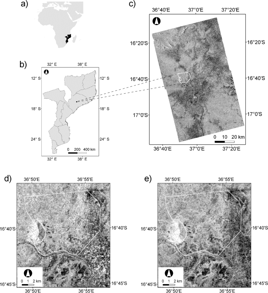
2. Background and Study Area

The study area is located in the central region of Mozambique, Zambézia province, district of Lugela, near the village of Mocuba (Figure 1) (16°04′S–17°16′S, 36°33′E–37°28′E). The climate is sub-humid, according to the Thorntwaite climate classification system. The dry season extends from March to November, the average annual precipitation ranges from 850 mm to 1,300 mm and the mean temperature from 20 °C to 27 °C.
The region is mostly covered by Miombo forests, the most extensive tropical savanna woodland formation of Africa that extends across some of the world’s poorest countries [22] and directly supports the livelihoods of the local populations. The main economic activity in the Lugela district is agriculture, which accounts for around 82% of the economically active population, followed by hunting activities, wood collection (for construction timber, charcoal production and domestic fuel), collection of medicinal plants, palm wine extraction, sand extraction and fishing. During the past year, an energy company has been making some efforts to understand and support the livelihoods of local populations (who are still recovering from decades of war) in the context of a suitability assessment for the production of biofuel in the region. For that and as a first step, lacking infrastructures were built, namely roads and a bridge. A detailed assessment was carried out to determine the impact of a plantation with Jatropha curcas L. (a non-edible plant whose oil-rich seeds can be processed into biodiesel). The best location for the installment of the plantation in a ∼10,000 ha parcel of land was decided, complying with the sustainability criteria listed in the Directive 2009/28/EC of the European Parliament [24]. Under this Directive, the energy from biofuel cannot be derived from raw material obtained from land with a high carbon stock. Therefore, all continuously forested areas, i.e., land spanning more than one hectare with trees higher than five meters and a canopy cover of more than 30% could not be used as plantation areas, and evidence of the low carbon stock of the area with a canopy cover between 10% and 30% before conversion must be provided, thus contributing to the sustainable management (social and environmental) of this area of interest and, ultimately, contributing to the company’s carbon emissions reduction targets as a whole. The ∼10,000 ha parcel of land was therefore divided into different classes of land use and tree canopy cover (see Section 3.1 for details) to assess the feasibility of the plantations and biofuel production in this area. This study focused on the areas with a tree canopy cover below the 50% threshold, corresponding to 16.5% of the total area.

3. Data

3.1. Field Measurements

Sampling was designed to accurately account for the total biomass C stocks in the selected carbon pools and was stratified using ancillary data provided from on-screen classification of very high spatial resolution satellite data (WorldView 2) images into four strata with different tree crown cover (0–10, 10–30, 30–40, 40–50%). A systematic grid of points with a random origin was created covering the Miombo area with a tree canopy cover between 10% and 50% in the ∼10,000 ha parcel of land and used as a basis for plot location. A total of 51 circular plots with a 20-m radius were randomly selected over the grid and measured during a field campaign that took place in July and August 2011. At the plot level, the following data were recorded: geographic coordinates (with global positioning system, GPS), physiographic location, dominant aspect and slope. At the stand level, data recorded included the tree crown cover, litter layer, down dead wood, sampling of live non-tree vegetation (herbaceous plants and shrubs) and soil organic carbon, up to 30 cm. At tree level, species were identified, tree vitality classified and diameter at breast height (DBH) measured for all trees with a DBH greater than 5 cm.
Several C pools were estimated, namely the live above- and below-ground tree biomass and soil biomass. Root biomass (i.e., BGB) was not measured in the field, but assessed through a root-to-shoot ratio (R:S = 0.42) reported by Ryan et al.[25]. As this study focuses only on the estimation of forest AGB, all the other pools measured in the field (down dead wood, litter, soil) were not included in the following sections.
Several allometric equations were identified for estimating the AGB of trees; two are Miombo specific, reported in (1) Ryan et al.[25] and (2) Chidumayo [26] and the other two, for dry tropical forests, reported in (3) Chave et al.[27] and (4) Brown et al.[28].
(1)
The allometric equation developed by Ryan et al.[25] for estimating the C content of the AGB of each tree is given by Equation (1):
ln ( B stem ) = 2.601 ln ( D B H ) 3.629
where Bstem is the tree AGB (kg·C), DBH the diameter at breast height (cm) and ln the natural logarithm. C content was estimated by using a conversion factor of 0.47 [25]. The coefficient of determination (R2) of this fitted equation was 0.93 and the root mean square error was 0.52 ln(kg C) (n = 29).
(2)
Chidumayo [26] developed relationships that relate AGB as a function of DBH (in Williams et al.[29]) and are presented in Equations (2) and (3):
A G B = 7.48 + 3.01 D B H ( for D B H < 10 cm )
A G B = 203.37 + 20.02 D B H ( for D B H > 10 cm )
where AGB is in kg and DBH in cm.
(3)
Separate equations for the estimation of AGB as a function of climate and primarily the mean monthly evapotranspiration (ET) and rainfall (R) were developed by Chave et al.[27], with these being wet (ET > R in less than one month per year), moist (ET > R more than one month and less than five months per year) and dry (ET > R more than five months per year) forests. These criteria basically defined the extent of the growing period (when R is greater than ET) as a proportion of the year and on a monthly basis. Thus, the same criteria can be rearranged in terms of growing period (GP) as (i) wet (GP > 11/12), (ii) moist (11/12 > GP > 7/12) and (iii) dry (GP < 7/12). Using the GP dataset produced by Silva et al.[14], the forests of the study area could be considered as belonging to the dry category. Therefore, Equation 4 was used:
A G B = ρ e ( 0.667 + 1.784 ln ( D B H ) + 0.207 ( ln ( D B H ) ) 2 0.0281 ( ln ( D B H ) ) 3 )
where AGB is in kg, ρ is the wood specific density (oven-dried on a green volume basis, g·cm−3) and DBH is in cm.
(4)
Brown et al.[28] developed another equation (Equation (5)) for the dry forest life zone:
A G B = 34.4703 8.0671 D B H + 0.6589 D B H 2
where AGB is in kg and DBH is in cm. The model has a R2 = 0.67 and a mean square error of 0.02208 (n = 32).
In the end, tree AGB were computed as the arithmetic mean of the values derived from these four equations.

3.2. ALOS PALSAR

The Japan Aerospace Exploration Agency (JAXA) launched ALOS on 24 January 2006, placing the satellite in a polar, sun synchronous orbit at ∼700 km and ensuring a 46-day repeat cycle. PALSAR is one of the instruments onboard ALOS, which is an enhanced version of the Japanese Earth Resources Satellite (JERS-1) SAR instrument [30]. PALSAR has a center frequency of 1,270 MHz (23.6 cm, i.e., L-band) and a chirp bandwidth of 14 MHz and 28 MHz. The instrument operated in five different observation modes, (i) Fine Beam Single (FBS), (ii) Fine Beam Dual (FBD), (iii) Polarimetric (PLR), (iv) ScanSAR and (v) Direct Transmission (DT). However, data acquired in the FBD mode was used, with these providing HH/HV or VV/VH polarizations (14 MHz bandwidth). Whilst 18 alternative off-nadir viewing angles were available (from 9.9° to 50.8°), only that acquired at 34.3° (HH and HV) polarization) were selected by JAXA and used with these acquired in ascending node with a 70 km swath width. Rosenqvist et al.[30] provide a complete reference and description of the ALOS PALSAR sensor.
The European Space Agency (ESA) catalogue was used to select the two ALOS PALSAR FBD (HH and HV polarizations) scenes required to cover the entire study area. The data were acquired on 21 June 2010, with an off-nadir angle of 34.3° (ascending orbits) (Figure 1), and were provided by ESA in level 1.1 (single look complex, SLC). The SARScape software (version 4.3.001) produced by Sarmap SA ( http://www.sarmap.ch) was used for all ALOS PALSAR processing, which followed standard SAR processing (e.g., [3134]). Prior to geocoding, the SLC data were converted to multi-look intensity (MLI) format. To obtain approximately square pixels in ground range coordinates, a multi-look factor of 1 in range and 5 in azimuth was used. The resulting MLI data was geocoded to a ground resolution of 15 m (both in range and azimuth). No filtering for speckle noise reduction was performed. The geocoding of the MLI data, which refers to a transformation from the slant-range/azimuth geometry to map projection geometry, was performed to obtain geocoded terrain corrected (GTC) images. GTC requires a digital elevation model (DEM), which was applied to the scenes acquired over the study area. A 90 m DEM retrieved from the Shuttle Radar Topography Mission (SRTM) over the study area was used. This DEM (version 4) was provided by the International Centre for Tropical Agriculture (CIAT) and obtained from the European Commission (EC) Joint Research Center (JRC). To obtain GTC images, a backward solution is usually implemented, which considers an input DEM, which is used to convert the positions of the backscatter elements into slant range image coordinates. The transformation of the three-dimensional object coordinates—given in a cartographic reference system—into the two-dimensional row and column coordinates of the slant range image, is performed by rigorously applying the Range and Doppler equations [32]. In case of precise satellite orbits, which is the case of ALOS, the geocoding process is run in a fully automatic way, and pixel accuracy can be achieved. Please refer to Meier et al.[32] for a more comprehensive description of the GTC method used in SARScape.
Radiometric calibration was carried out by following the radar equation law and involved corrections for the scattering area, the antenna gain pattern and the range spread loss [35,36]. A DEM is required to properly determine all required geometric parameters of the radar equation, so the calibration is performed during the data geocoding step, where the required parameters were already calculated. The calibrated value is a normalized dimensionless number (linear units, m2·m−2), and the corresponding value in the dB scale was generated by applying 10log10 of the linear value and was generated as gamma nought (γ°). Even after a rigorous radiometric calibration, backscattering coefficient variations are clearly identifiable in range direction and in presence of topography, which requires a radiometric normalization. These variations are an intrinsic property of each imaged object and, thus, might be compensated, but it may not be corrected in absolute terms. In this study, a cosine correction method was applied, which was based on a modified cosine model [31] and applied to the backscattering coefficient to compensate for range variations. After the two scenes had been geocoded, they were combined to create a mosaic. Figure 1c shows the mosaic of the two ALOS PALSAR FBD geocoded scenes over the study area.

3.3. Extraction of ALOS PALSAR FBD Data at Field Plot Locations

Each plot measured in the field had a 20 m radius. Although the coordinates of each plot center were collected with GPS, there are always positional errors, especially when differential corrections are unavailable (errors up to 8–10 m are common). Although pixel accuracy can be achieved with ALOS PALSAR data geocoding (15 m ground pixel spacing), some error will always be present. Therefore, to compensate for these two sources of position errors, a buffer around each plot center with a 50 m radius was created. The buffer was selected as anything larger would have impinged on areas that were not homogeneous in terms of the plot tree canopy cover. All ALOS PALSAR pixels inside each 50 m buffer around each plot center were extracted, with several metrics computed (mean, minimum, maximum and standard deviation) and used to establish relationships with the AGB at the plot level. As the original ALOS PALSAR FBD mosaic had a 15 m spatial resolution and the buffer around each plot center was set to 50 m, then the extracted values per plot were those located approximately on a 6 × 6 pixel window size centered on each plot center, thus extracting the data in a 90 × 90 m window.
To assess the amount of speckle of the processed ALOS PALSAR FBD MLI data (15 m ground resolution), the equivalent number of looks (ENL) (Equation (6)) (e.g., [33,34]) was estimated over a set of 30 Miombo homogeneous regions of interest spread over the study area:
E N L = μ 2 / σ 2
where μ and σ2 are the mean and variance of the backscatter intensity values (original scale). The estimated ENL mean values were 5.26 and 4.91 for the HH and HV polarizations, respectively. These values are approximately the same as the number of looks used to produce the MLI data, i.e., 1 look in range and 5 look in azimuth, thus resulting in a 5 look image, meaning that the amount of speckle anticipated during multilooking is comparatively the same as that estimated by Equation (6). However, as mentioned above, the ALOS PALSAR FBD data extracted per plot were equivalent to extracting data located on a 6 × 6 pixel window size centered on each plot center. Therefore, the amount of speckle present in the ALOS PALSAR FBD data used to model AGB should be that of the ALOS PALSAR FBD data averaged to a 90 m spatial resolution. The ENL corresponding to this ALOS PALSAR FBD data were estimated, using the same set of 30 homogeneous areas and the mean values were 48.86 and 37.82, for the HH and HV polarizations, respectively. It shows that the amount of speckle was substantially reduced by spatially averaging the ALOS PALSAR FBD data.

4. Methods

4.1. Contribution of Different ALOS PALSAR Polarizations and Metrics

Several scatterplots were produced to display and evaluate the strength of the relationship between ALOS PALSAR backscatter intensity (γ°) and AGB data estimated from field data. ALOS PALSAR backscatter intensity (γ°) for the HH and HV polarizations were displayed against AGB data. As the ALOS PALSAR data were extracted on a 50 m radius of each plot center, then several metrics were computed, namely, (i) mean, (ii) minimum, (iii) maximum and (iv) standard deviation. Also, the coefficient of correlation (R) between the ALOS PALSAR metrics and the AGB was computed, either using parametric (Pearson’s R) and non-parametric (e.g., Spearman’s rank R) approaches [37].

4.2. Regression with Stochastic Gradient Boosting (SGB) and Bagging SGB (BagSGB)

Traditionally, the attempt of explaining a given variable (dependent variable) as a function of one or more variables (predictor or independent variable(s)) has relied on parametric statistical models, such as linear (simple or multiple) regression models. These models have several assumptions, including normal distribution of errors and variables, as well as homoscedasticity (e.g., [38]). However, in the past decades and largely because of problems presented by large arrays of data, several other methods and algorithms have been developed, which are commonly referred to as machine learning methods. These methods have a large scope of application, from prediction (e.g., [39,40]) to classification (e.g., [41,42]) problems and can have different formulations (e.g., neural nets, ensembles of trees, support vector machines). A comprehensive review of these methods can be found in Hastie et al.[38].
SGB [43,44] originated from the decision tree theory (e.g., [38,45]). Decision tree theory relies on partitions of the space of all possible predictor variables. Starting with the whole predictor space (at the root of the tree), the space is successively split using a series of rules such that, in the end, each terminal node of the tree is assigned to the most probable response class (classification trees) or the mean response in that node (regression trees) [45,46]. Some advantages over traditional parametric classification methods include the non-parametric nature of the classifier, quantification of variable importance, disclosure of non-linear and hierarchical relationships between predictor variables, and acceptance of missing values [47,48]. However, classification and regression trees are sensitive to small perturbations in the training data, which may originate large changes in the resulting outputs [49]. Therefore, these unstable methods can have their accuracy improved with perturbing and combining techniques. These generate multiple perturbed versions of the classifier (a.k.a., ensemble or committee) and combines them into a single predictor [50]. These methods can be divided into two types: those that adaptively change the distribution of the training set based on the performance of previous classifiers (e.g., boosting) and those that do not (e.g., bagging) [51].
SGB [43,44] combines both the advantages of bagging and boosting and can be used in regression and classification problems (e.g., [5255]). It typically uses a base learner (in our case, binary decision trees) and constructs additive regression (or classification) models by sequentially fitting the chosen base learner to current “pseudo”-residuals by least squares at each iteration using a random fraction of the training data without replacement [44]. This process has been shown to substantially improve the prediction accuracy and execution speed, making the approach resilient to overfitting [44]. Furthermore, Suen et al.[56] demonstrated that building and combining (by averaging in the case of regression) several SGB models on samples randomly drawn with replacement from the original training dataset (bootstrap sample) performed significantly better than a unique SGB model and concluded that it was accomplished by variance reduction. Therefore, two approaches were followed, (i) generate a SGB model from the original training dataset and (ii) generate several SGB models fitted to bootstrap samples (with replacement) of the original training dataset that were then combined by averaging. This allowed us to compare SGB against bagging SGB (BagSGB).
Model fitting under SGB has a number of options that were tested to select the best model. This was done by developing in-house R code [57] to implement a loop using Ridgeway’s R gbm package [58] and Elith et al.[40] R code. These options include: (i) distribution (Gaussian, i.e., the loss function, whose measure of deviance to be minimized is the mean squared error), (ii) bagging fraction (i.e., the random fraction of the training data that is randomly selected to build each decision tree; 0.5, 0.6, 0.7, 0.8 and 0.9), (iii) tree complexity (i.e., the number of nodes in each decision tree; 1, 2, 3, 4, 5, 7 and 9) and (iv) shrinkage rate (i.e., controlling the learning rate of the algorithm; 0.01, 0.005, 0.0025, 0.001 and 0.0005) [58]. Therefore, the selection of the best SGB model is the result of evaluating 175 candidate individual SGB models (5 bagging fraction values × 7 tree complexity parameters × 5 shrinkage rate values). Elith et al.[40] referred to the fact that small shrinkage rates result in a smaller contribution of each tree and, therefore, are more directed at building a model that will provide a more consistent estimate of the dependent variable; as a rule of thumb, they indicate that, as a minimum, models should be fitted with 1,000 trees. Accordingly, to select the best SGB model out of the various candidates, we selected the model that had the lowest 10-fold cross-validated deviance (i.e., lowest mean squared error), given that a minimum of 1,000 trees were used to generate that model.
This procedure was carried out for each bootstrap sample of the original training dataset when generating the BagSGB model. We used 25 bootstrap samples to build a BagSGB model, as Breiman [49] suggests that a higher number of replicates tend not to produce a significant test set error reduction. The final model (bagging SGB or BagSGB) was built by averaging the predictions from the 25 selected SGB models fitted to the bootstrap samples. Also, as each predicted observation is the result of averaging over a set of 25 bootstrap samples, it allows also building a measure of prediction variability. The coefficient of variation (CV) (e.g., [37]), calculated as the standard deviation of a predicted observation divided by the corresponding mean value, was used as a measure of assessing the uncertainty associated with each prediction.
AGB was chosen as the dependent variable, and the mean, minimum, maximum and standard deviation of the ALOS PALSAR HH and HV backscatter intensity values extracted for each plot (50 meters buffer around each plot center) were selected as independent variables. The number of pixels that were used to compute those metrics ranged from 28 to 37, the variation being dependent on the plot location regarding the 15 m ALOS PALSAR data.
The SGB and BagSGB models were compared using a traditional bias and variance decomposition of the root mean square error (RMSE) (Equations (79)). A 10-fold cross validation approach was followed, as the number of observations was not large enough to evaluate model performance with an independent subset (e.g., [38]).
R M S E = 1 n i = 1 n e i 2 = σ 2 + b 2
where RMSE is the model root mean square error, ei the error (difference between the observed and predicted values) of the ith observation, σ2 the error variance, b the error bias and n the number of observations;
σ 2 = 1 n i = 1 n ( e i e ¯ ) 2
where ē is the mean error;
b = 1 n i = 1 n e i

4.3. C Stocks and Comparison with Published Biomass Maps

Mean AGB and C stocks per tree canopy cover classes under 50% were estimated, as well as the total AGB and C stock in the Miombo forests of the broader study area (∼10,000 ha). The default carbon fraction of dry matter of 0.47 obtained from the Intergovernmental Panel on Climate Change [59] was used to convert Miombo forest AGB to C content. This default value is consistent with the dry mass fraction determined by Ryan et al.[25] with subsamples from both the trunk and branches of 19 trees from a Miombo region in central Mozambique.
A comparison with published biomass maps, especially when derived from distinct data sources, is important, namely to compare and assess differences in the AGB and C stocks estimates in a same ecosystem and region. For that, two published maps were selected: Baccini et al.[60] and Saatchi et al.[12]. Baccini et al.[60] mapped AGB across tropical Africa (1 km spatial resolution) using an ensemble of regression tree-based models (random forests) that relate in situ measurements with data acquired by the Moderate Resolution Imaging Spectroradiometer (MODIS) onboard NASA’s Terra and Aqua satellites between 2000 and 2003; a cross-validation approach showed that the model explained 82% of the variance in AGB, corresponding to a RMSE of 50.5 Mg·ha−1 (for AGB values between 0 and 454 Mg·ha−1). Saatchi et al.[12] mapped forest C stocks, AGB plus below-ground biomass (BGB), in the pan-tropical belt (∼1 km spatial resolution) around the year 2000 using a data fusion algorithm based on the maximum entropy approach (MaxEnt) to model field-based measurements as a function of data acquired by the Geoscience Laser Altimeter System (GLAS) onboard the Ice, Cloud and land Elevation Satellite (ICESat) and extrapolating to the landscape using data from other optical and microwave sensors; the prediction variability ranged from ±6% to ±53% on a pixel basis, but when scaling-up to project- and country-scales, the errors decreased to ±5% and ±1%, respectively.
The uncertainty at the study area level (UP) was estimated using the error propagation approach (Equation (10)) (e.g., [61]), which is the same equation used to assess overall uncertainty in REDD projects and national greenhouse gas inventories [59]:
U P = i = 1 N ( A G B i U i ) 2 i = 1 N A G B i
where AGBi and Ui are the forest AGB and uncertainty at the ith pixel, respectively, and N the number of pixels in the area being assessed.

5. Results and Discussion

5.1. Forest AGB from Field Data

As mentioned in section 3.1, the four selected allometric equations were used to produce an estimate of each tree AGB and were subsequently averaged to produce an estimate of AGB of each measured tree. Table 1 depicts the average AGB C stock per tree canopy cover class.

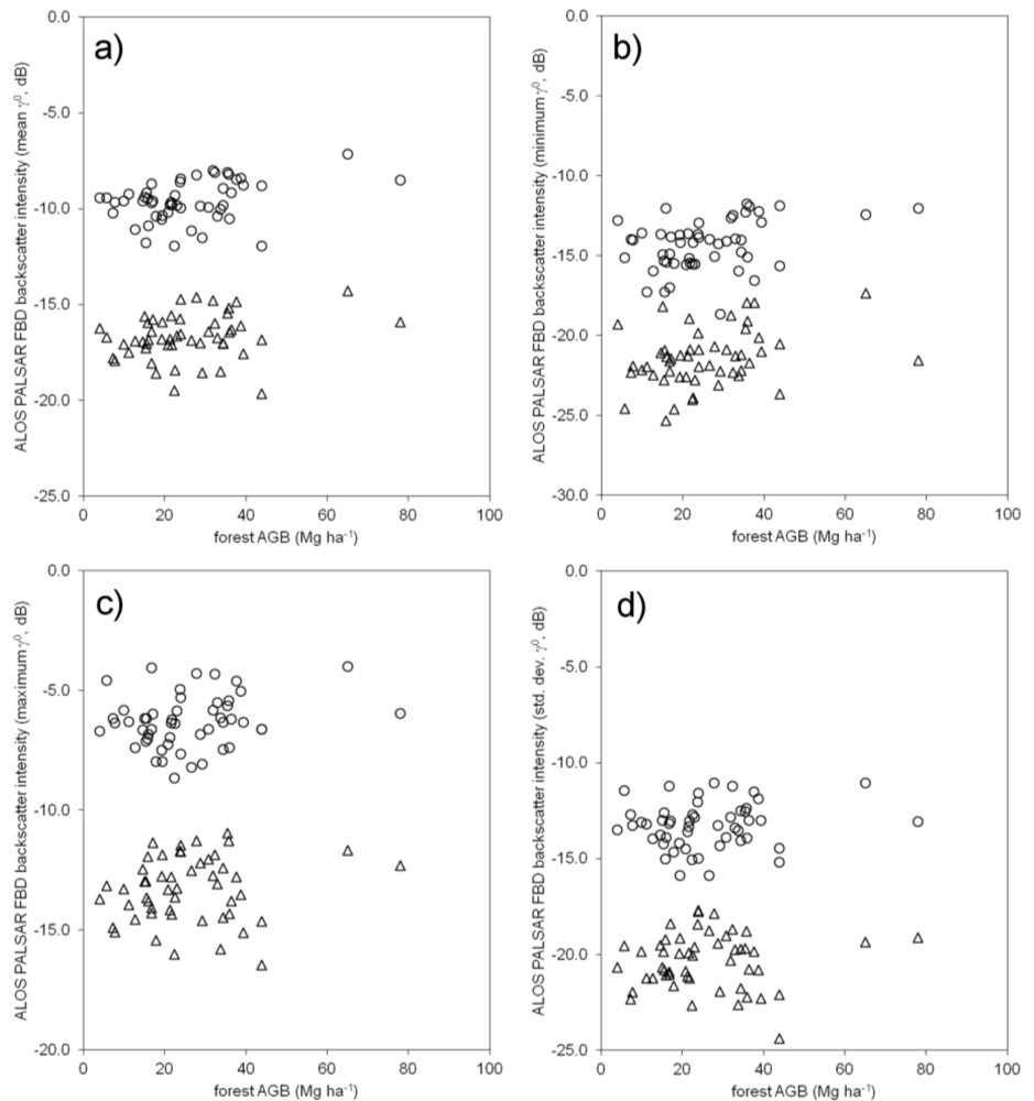
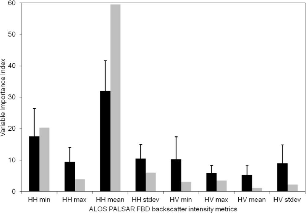
5.2. Contribution of ALOS PALSAR Polarizations and Metrics

The relationship between ALOS PALSAR backscatter intensity data (HH and HV polarizations) and forest AGB data is shown in Figure 2. The mean, minimum, maximum and standard deviation were computed based on the ALOS PALSAR backscatter intensity data extracted over a 50 m radius of each plot center. The mean and the minimum values are those displaying a less scattered relationship with the forest AGB. This was further confirmed with the computation of the coefficient of correlation between forest AGB and the four metrics derived from the ALOS PALSAR data (Table 2). For a significance level of 0.05, the significant coefficients of correlation were those between forest AGB and the minimum associated with the HH and HV polarizations and the mean associated with the HH polarization. The sampled plots were located in Miombo areas with tree canopy cover between 10% and 50%, encompassing some areas with a large proportion of bare soil and/or herbaceous vegetation and low tree density. Therefore, it is expected that the backscatter intensity reaching the SAR sensor was influenced greatly by this land cover types, especially influenced by their surface roughness (bare soil) and moisture content (bare soil), two of the factors greatly influencing the backscatter response from L-band SAR sensors. Also, with such low tree canopy cover, it is expected that the L-band radiation interacts with the tree trunks, thus originating a better response with the HH polarization.

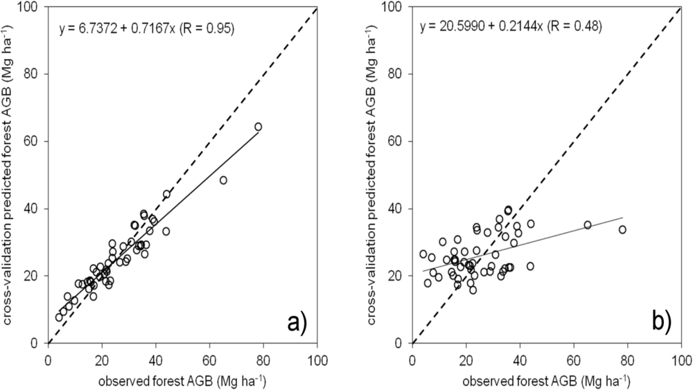
5.3. BagSGB Modeling

The final BagSGB model was the result of combining the 25 SGB models built from the corresponding bootstrap samples of the original training dataset. The forest AGB values predicted from the 10-fold cross-validation of each of the 25 models were aggregated (averaged) and the corresponding statistics calculated (Table 3). The comparison between observed and cross-validation predicted forest AGB values is displayed in Figure 3(a). Each cross-validation predicted forest AGB value was the result of averaging between 16 and 36 times, as each bootstrap sample was built with replacement. A close correspondence (R = 0.95) between observed and cross-validation predicted forest AGB values was identified, although the AGB above 40 Mg·ha−1 was slightly underestimated. However, there is no evidence that it is a trend consistent with L-band SAR saturation, as only four plots have AGB values higher than that value. As a comparison, the same combination of parameters (i.e., distribution, bag fraction, tree complexity and learning complexity) was tested to build the best SGB model fitted to the original training dataset. This model was based on 4,700 trees, resulting from a bag fraction of 0.8, a learning rate of 0.0005 and a tree complexity of 2. The 10-fold cross-validation results performed less well than those resulting from the application of an ensemble of SGB models (i.e., a BagSGB model). The cross-validation RMSE of this model was 12.04 Mg·ha−1(5.03 Mg·ha−1 in the BagSGB model), the variance 144.81 (24.96 in the BagSGB model), the error bias −0.32 Mg·ha−1 (0.58 Mg·ha−1 in the BagSGB model) and the linear coefficient of correlation (R) between observed and cross-validation predicted AGB values was 0.48 (0.95 in the BagSGB model). Figure 3(b) shows the scatterplot between observed and cross-validation predicted forest AGB values for this SGB model. The error bias is approximately the same; therefore, the RMSE decrease (from 12.04 to 5.03 Mg·ha−1) was a consequence of variance reduction from 144.81 in the SGB model to 24.96 in the BagSGB model. This is in agreement with the results of Suen et al.[56] already mentioned in Section 4.2.
To evaluate the degree of prediction variability associated with the fitted BagSGB model, the coefficient of variation of the forest AGB was calculated, using the average and standard deviation values of forest AGB obtained during the 10-fold cross-validation of this fitted model. The relationship between the 10-fold cross-validation predicted forest AGB and corresponding coefficient of variation values is shown in Figure 4. The coefficient of variation is higher for lower forest AGB values, decreasing until forest AGB values around 20 Mg·ha−1 and then increasing slightly again for values above 50 Mg·ha−1. However, these higher values of the forest AGB coefficient of variation are not that evident in the relationship between observed and cross-validation predicted forest AGB values (Figure 3(a)), thus suggesting that the averaging process inherent to a BagSGB model results in a reduced variance. Nevertheless, we acknowledge that some bias may have been introduced in the fitted BagSGB model as a consequence of using bootstrap samples of the original training dataset. The bootstrap samples were built with replacement, so each bootstrap sample will have at least duplicates of some observations (i.e., plots). As the evaluation of the BagSGB model was performed by a 10-fold cross validation approach, one cannot guarantee that the same observation is not present in the training subset (9/10-fold) and in the testing subset (1/10-fold), hence the cross-validation statistics may be skewed and, as such, resulted in overoptimistic metrics of model validation.
The importance of each independent variable for the fitted BagSGB model is displayed in Figure 5. The score of each variable is the result of averaging the scores among the 25 SGB models, which composed the final BagSGB model. The most important variable is the mean value of the ALOS PALSAR FBD HH backscatter intensity, followed by the minimum value of the ALOS PALSAR FBD HH backscatter intensity. The other tested variables have lesser importance for the fitted SGB model. The standard deviation of the variable importance index for each metric is rather high, thus suggesting that the metrics used to build the 25 SGB models that compose the final BagSGB model could have had different weights, depending of the data structure (i.e., the observations that were randomly selected with replacement for each bootstrap sample). However, these scores confirm the results presented in Figure 3 and Table 2, as these were the variables that had a less scattered relationship with forest AGB and had coefficients of correlation significant at a significance level of 0.05. As a comparison, the variable importance score is also indicated for the variables that were used to build the SGB model using the original training dataset. It shows that the most important variables are the same as for the BagSGB model, but the importance of the mean value of the ALOS PALSAR FBD HH backscatter intensity is much higher when comparing with the BagSGB model. This could also be an indication that the main scattering pathways influencing the backscatter intensity are those related to the HH polarization, which are mainly trunk-ground corner reflector scattering, canopy-ground scattering and scattering from the ground after transmission through the canopy (e.g., [62]).
On the basis of its better performance in the cross-validation assessment, the BagSGB was applied to the entire study area. The ALOS PALSAR FBD backscatter intensity data used to build the model were extracted in a 50 m buffer around each plot center ,with this being equivalent to a spatial resolution of approximately 100 m. Therefore, to create the forest AGB map of the study area, the original ALOS PALSAR FBD backscatter intensity data at 15 m spatial resolution was necessarily aggregated to a 90 m spatial resolution, and the minimum, maximum, mean and standard deviation values were computed. Also and for displaying purposed, the continuous AGB map was transformed into a five-class map (Figure 6). As mentioned in Section 4.2, the type of algorithm used allowed the production of a map displaying the prediction variability in each pixel, by computing the coefficient of variation (%) on a pixel-by-pixel basis and for the same reasons was converted into a five-class map (Figure 7). As mentioned above, although the 10-fold cross validation procedure that was implemented may have resulted in overoptimistic values of model assessment, the prediction variability at the pixel level provides additional and complementary information regarding the spatial distribution of the model error that could be used to assess its applicability to new observations.

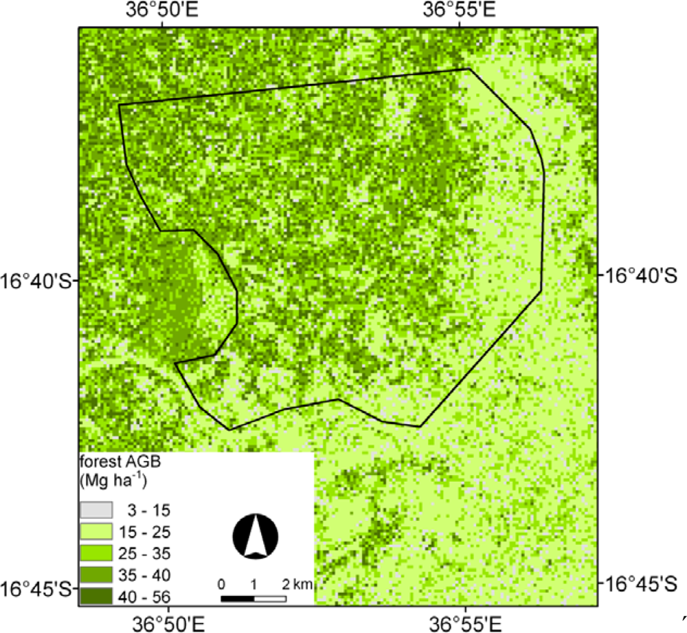
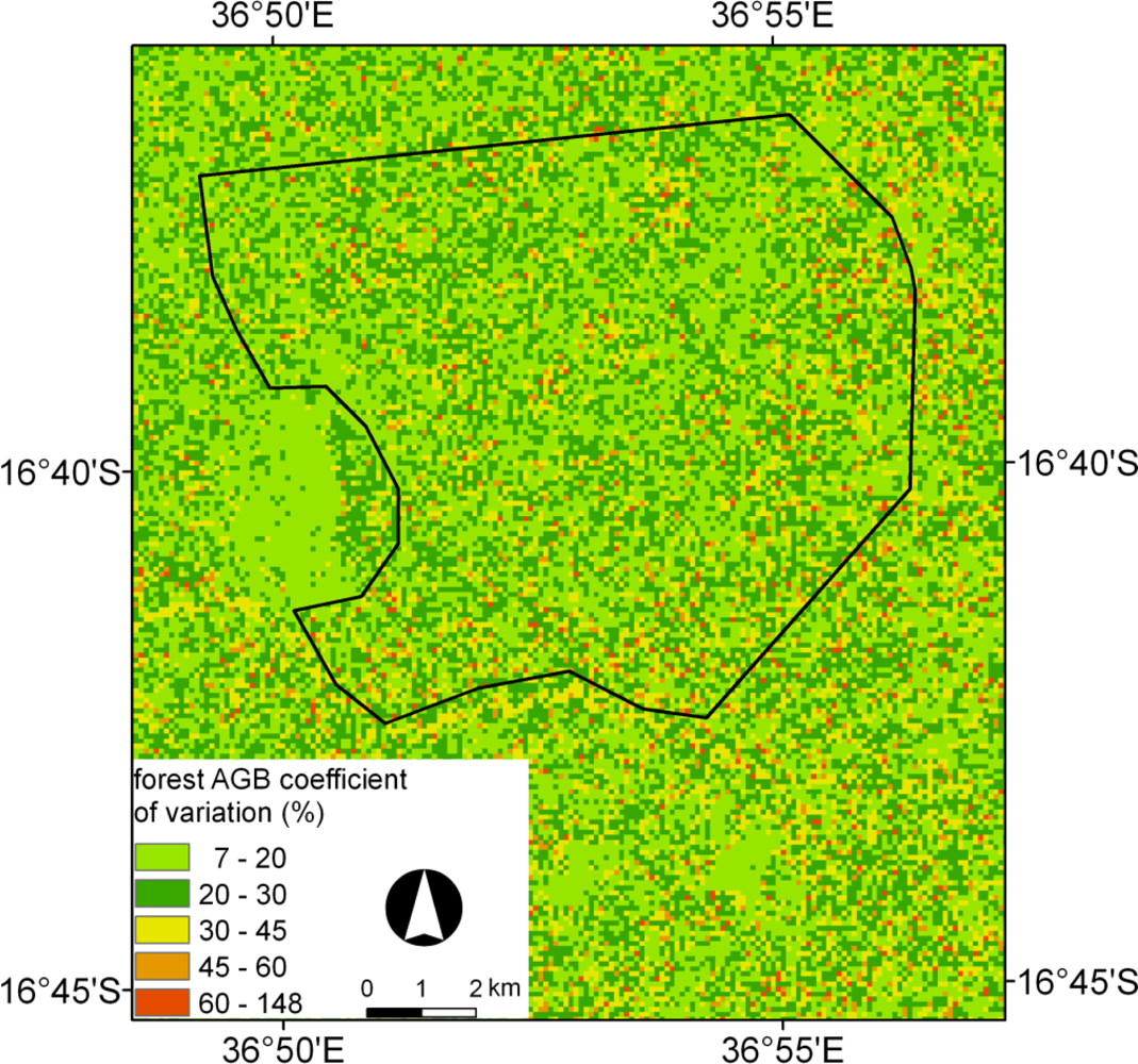
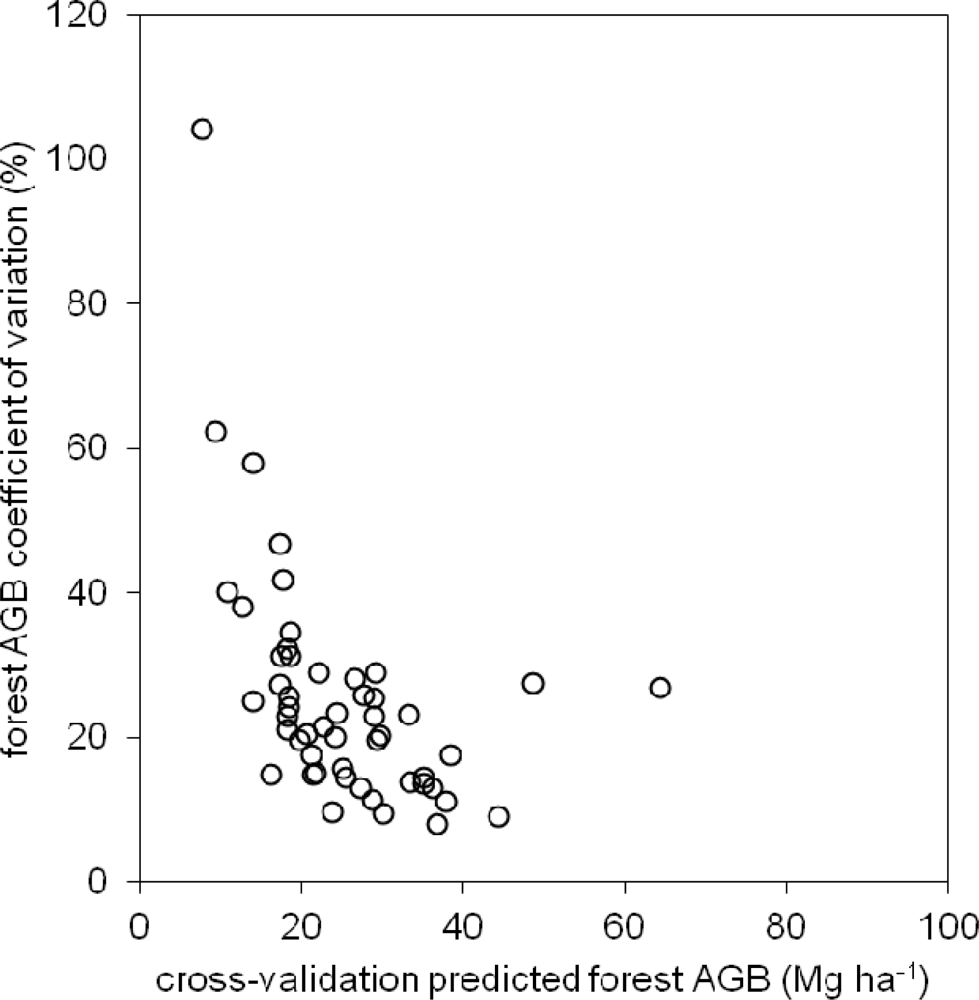
5.4. C Stocks and Comparison with Published Biomass Maps

Mean forest AGB and derived C stocks, as well as uncertainty per tree canopy cover class in the study area (∼10,000 ha) were calculated on the basis of the forest AGB map produced in this study in the same manner as in the work of Baccini et al.[60] and Saatchi et al.[12]. Differences in the time frame of each study (2008 for this study, 2000–2003 for Baccini et al.[60] and early 2000s for Saatchi et al.[12]) were not considered nor addressed here. The forest AGB carbon stock obtained for the entire study area from this study (143,444 Mg·C) is very different from the values obtained with data from Baccini et al.[60] (498,570 Mg·C) and Saatchi et al.[12] (405,986 Mg·C). The mean AGB obtained with the data from this study is 30.6 Mg·ha−1, while in Baccini et al.[60], it is 106.3 Mg·ha−1 and in Saatchi et al.[12], 86.6 Mg·ha−1. Mitchard et al.[63] on their evaluation of the data published by Baccini et al.[60] used an independent dataset of 1,154 field measurements, obtained in 16 African countries and concluded that large errors were associated with this AGB map; more significantly for our study, there was large underestimation in forests with higher AGB and overestimation in woodland savannas, resulting in a RMSE of 145 Mg·ha−1. However, Saatchi et al.[12] also reported higher values than those reported here. As mentioned in Section 3.1, in our study, only the area with a tree canopy cover between 10% and 50% was sampled for forest AGB estimation, and therefore, it is not unexpected that the derived C stock and mean AGB are lower than those reported in studies using field data spanning the entire tree canopy cover range. Also, it is important to note that the Miombo forests are diverse in terms of tree canopy cover and, therefore, C content. For example, Glenday [64] reported an average forest AGB value of approximately 92 Mg·ha−1 for Brachystegia sp. dominated dry forests in Kenya. Malimbwi et al.[65], using field data collected in the Miombo woodlands of Tanzania, reported an average forest AGB value around 18 Mg·ha−1. Ryan et al.[25] estimated an average forest AGB value of 45 Mg·ha−1 for a Miombo woodland in Mozambique. Shirima et al.[66] measured several plots in Miombo forests of Tanzania and estimated a mean forest AGB value of approximately 48 Mg·ha−1. The study of Ryan et al.[25] was carried out in areas of Miombo formations similar to those addressed in the present study and the estimated mean AGB was 45 Mg·ha−1; a value that compares with the 31 Mg·ha−1 estimated during this study. The difference can probably be related to the 10–50% threshold of the measured Miombo in this study.
The estimated forest AGB uncertainty at the study area level was 0.21% (coefficient of variation) in this study and 2.82% (error) in Saatchi et al.[12]. The values of uncertainty on a pixel basis ranged from 10–119% (mean = 25%) and 21–31% (mean = 27%) in this study and in Saatchi et al.[12] respectively. Although higher on a pixel level, the values decrease substantially when the measure of uncertainty is obtained at a study area level. This is also the case in Saatchi et al.[12].
Furthermore, the mean forest AGB and the total C stocks were estimated for the subset of the study area with a tree canopy cover between 10% and 50% (1,157 ha), which was the area sampled during the field campaign that took place in the 2011 dry season. The estimates are depicted in Table 4 by tree canopy cover classes. Similarly as for the results presented in Table 4, the estimates of mean AGB and total AGB C stock per tree canopy cover class derived from this study are substantially lower than those estimated in Baccini et al.[60] and Saatchi et al.[12].
Romijn [67] concluded that the land use change associated with the introduction of Jatropha curcas L. in Miombo savanna woodlands will only have a positive feedback (i.e., atmospheric carbon sequestration) when introduced in wastelands or severely degraded lands; however, he acknowledges that the data used in his study have a high degree of uncertainty, especially due to substantial regional and local variations in soil, biomass and climate characteristics. Nevertheless, for industry and for the purpose of complying with the objectives of environmental sustainability in biofuel plantations, it is important to guarantee that the C content of the areas to be converted is sufficiently low at the start, so that the biofuel produced actually corresponds to savings in carbon emissions when compared to fossil fuels, and thus, it is effectively contributing to the countries’ and companies’ renewable energy targets. Given uncertainties in carbon estimations, good practice demands that a conservative approach be applied. Thus, an accurate enough, expedient and cost effective method for spatially explicit carbon quantification whose performance risk is systematic underestimation may constitute a helpful planning tool.
When dealing with international funds for performance based payments to developing countries in the context of REDD, the use of the conservativeness principle for estimating emissions from deforestation and forest degradation is always required. In such cases, establishing a reference emission level using a conservative carbon stock is mandatory. Ryan et al.[68] in their study in areas of Miombo savanna woodland located in central Mozambique concluded that deforestation activities were not particularly occurring in high biomass areas. Therefore, by using estimates of forest AGB exclusively from data retrieved from plots that had a tree canopy cover between 10% and 50%, we could actually be encompassing the areas more prone to deforestation and, therefore, provide more conservative estimates of forest AGB for REDD projects. Additionally, the methodology used in this study could be easily adapted to produce spatial conservative estimates of C stocks in the AGB pool. The methodology uses n (in this case n = 25) SGB models and then averages them to estimate the AGB at the pixel level. Therefore, a conservative estimate of AGB at a given pixel could be obtained by using a given percentile (lower than 50%) of the distribution of possible forest AGB values for that pixel. Alternatively, the coefficient of variation that is produced, also on a pixel-by-pixel basis, could be used to discount the value of the estimated forest AGB.

6. Conclusions

Consistent forest carbon monitoring methods are required at various levels, namely for developing countries who wish to address international conventions and to access carbon-based financial mechanisms associated with climate change mitigation. A method for reducing the uncertainty in the estimation of forest above-ground biomass (AGB) in Miombo savanna woodlands in southeast Africa (Zambézia province, Mozambique) has been presented. The advancement of this study relied on the use of a machine learning algorithm to establish a relationship between in situ forest AGB and L-band Synthetic Aperture Radar (SAR) backscatter intensity (gamma nought, γ°) data obtained from the Phased Array L-band SAR (PALSAR) sensor onboard the Advanced Land Observing Satellite (ALOS). This algorithm, bagging stochastic gradient boosting (BagSGB), is unique, as it allows also the production of spatial explicit estimates of prediction variability and an indication of the importance of each predictor variable. Estimates of forest AGB with a root mean square error (RMSE) of 5.03 Mg·ha−1 based on 10-fold cross validation were produced with this modeling approach. Also, the coefficient of correlation (R) between observed and predicted (from 10-fold cross validation) forest AGB values was 0.95. The variable contributing the most to this model was the mean backscatter intensity for the HH polarization, which was explained by the low tree canopy cover characterizing Miombo savanna woodlands, thus invoking scattering mechanisms associated with this polarization (e.g., trunk-ground scattering). Furthermore, it was recognized that the optimistic overall validation results (RMSE and R) might be a consequence of the 10-fold cross-validation procedure, especially when dealing with bootstrap samples that were drawn with replacement. Nevertheless, this algorithm was unique in producing estimates of prediction variability (coefficient of variation) on a pixel-by-pixel basis. These estimates ranged from 10 to 119% across the study area, with a mean value of 25%. This map of prediction variability (Figure 7) is a useful instrument to assess how well the model is predicting new observations.
One of the reasons for the observed disagreement between the mean forest AGB values and total forest AGB carbon (C) stocks generated from this study and those resulting from the two available forest AGB maps (i.e., [12,60]) could be related to the fact that only the forest areas with tree canopy cover between 10% and 50% were sampled for the collection of in situ data. Therefore, subsequent work will rely on sampling the Miombo areas with tree canopy cover greater than 50%, which will allow a better characterization of the Miombo savanna woodlands in the region and more in situ observations to produce an updated version of the BagSGB model.

Acknowledgments

This work was possible through the support of two projects: “Quantification of biomass in Miombo woodlands (Mozambique, East Africa) using radar and optical remote sensing data” (Ref. ESA C1P 9472) and “REGROWTH-BR - Remote sensing of regenerating tropical forests in Brazil: mapping and retrieving biophysical parameters” (Ref. PTDC/AGR-CFL/114908/2009). Galp Energia, S.A. is acknowledged for providing the field data and the ancillary maps and for funding the acquisition of the ALOS PALSAR data used in this study. The careful and insightful comments of two anonymous reviewers are particularly thanked.

References

  1. Pan, Y.; Birdsey, R.; Fang, J.; Houghton, R.; Kauppi, P.; Kurz, W.; Phillips, O.; Shvidenko, A.; Lewis, S.; Canadell, J.; et al. A Large and persistent carbon sink in the world’s forests. Science 2011, 333, 988–993. [Google Scholar]
  2. Le Quere, C.; Raupach, M.; Canadell, J.; Marland, G.; Bopp, L.; Ciais, P.; Conway, T.; Doney, S.; Feely, R.; Foster, P.; et al. Trends in the sources and sinks of carbon dioxide. Nat. Geosci. 2009. [Google Scholar] [CrossRef]
  3. Houghton, R.; Hall, F.; Goetz, S. Importance of biomass in the global carbon cycle. J. Geophys. Res.-Biogeosci. 2009, 114. [Google Scholar] [CrossRef]
  4. Gibbs, H.; Brown, S.; Niles, J.; Foley, J. Monitoring and estimating tropical forest carbon stocks: Making REDD a reality. Environ. Res. Lett. 2007, 2. [Google Scholar] [CrossRef]
  5. Campbell, B. Beyond Copenhagen: REDD plus, agriculture, adaptation strategies and poverty. Glob. Environ. Chang.-Human Policy Dimens 2009, 19, 397–399. [Google Scholar]
  6. Danielsen, F.; Skutsch, M.; Burgess, N.D.; Jensen, P.M.; Andrianandrasana, H.; Karky, B.; Lewis, R.; Lovett, J.C.; Massao, J.; Ngaga, Y.; et al. At the heart of REDD: A role for local people in monitoring forests. Conserv. Lett 2011, 4, 158–167. [Google Scholar]
  7. Herold, M.; Verchot, L.; Angelsen, A.; Maniatis, D.; Bauch, S. A Step-Wise Framework for Setting REDD+ Forest Reference Emission Levels and Forest Reference Levels; Center for International Forestry Research (CIFOR): Bogor, Indonesia, 2012. [Google Scholar]
  8. Mora, B.; Herold, M.; De Sy, V.; Wijaya, A.; Verchot, L.; Penman, J. Capacity Development in National Forest Monitoring: Experiences and Progress for REDD+; Joint Report by CIFOR and GOFC-GOLD: Bogor, Indonesia, 2012. [Google Scholar]
  9. Chambers, J.; Asner, G.; Morton, D.; Anderson, L.; Saatch, S.; Espirito-Santo, F.; Palace, M.; Souza, C. Regional ecosystem structure and function: Ecological insights from remote sensing of tropical forests. Trends Ecol. Evol 2007, 22, 414–423. [Google Scholar]
  10. Goetz, S.J.; Baccini, A.; Laporte, N.T.; Johns, T.; Walker, W.; Kellndorfer, J.; Houghton, R.A.; Sun, M. Mapping and monitoring carbon stocks with satellite observations: A comparison of methods. Carbon Balan. Manag. 2009, 4. [Google Scholar] [CrossRef]
  11. Lucas, R.; Armston, J.; Fairfax, R.; Fensham, R.; Accad, A.; Carreiras, J.; Kelley, J.; Bunting, P.; Clewley, D.; Bray, S.; et al. An Evaluation of the ALOS PALSAR L-Band Backscatter-Above Ground Biomass Relationship Queensland, Australia: Impacts of Surface Moisture Condition and Vegetation Structure. IEEE J. Sel. Top. Appl. Earth Obs. Remote Sens 2010, 3, 576–593. [Google Scholar]
  12. Saatchi, S.; Harris, N.; Brown, S.; Lefsky, M.; Mitchard, E.; Salas, W.; Zutta, B.; Buermann, W.; Lewis, S.; Hagen, S.; et al. Benchmark map of forest carbon stocks in tropical regions across three continents. Proc. Natl. Acad. Sci. USA 2011, 108, 9899–9904. [Google Scholar]
  13. Carreiras, J.M.B.; Vasconcelos, M.J.; Lucas, R.M. Understanding the relationship between aboveground biomass and ALOS PALSAR data in the forests of Guinea-Bissau (West Africa). Remote Sens. Environ 2012, 121, 426–442. [Google Scholar]
  14. Silva, J.M.N.; Carreiras, J.M.B.; Rosa, I.; Pereira, J.M.C. Greenhouse gas emissions from shifting cultivation in the tropics, including uncertainty and sensitivity analysis. J. Geophys. Res.-Atmos. 2011, 116. [Google Scholar] [CrossRef]
  15. Hall, F.; Bergen, K.; Blair, J.; Dubayah, R.; Houghton, R.; Hurtt, G.; Kellndorfer, J.; Lefsky, M.; Ranson, J.; Saatchi, S.; et al. Characterizing 3D vegetation structure from space: Mission requirements. Remote Sens. Environ 2011, 115, 2753–2775. [Google Scholar]
  16. Saatchi, S.; Halligan, K.; Despain, D.; Crabtree, R. Estimation of forest fuel load from radar remote sensing. IEEE Trans. Geosci. Remote Sens 2007, 45, 1726–1740. [Google Scholar]
  17. Popescu, S.; Zhao, K.; Neuenschwander, A.; Lin, C. Satellite lidar vs. small footprint airborne lidar: Comparing the accuracy of aboveground biomass estimates and forest structure metrics at footprint level. Remote Sens. Environ 2011, 115, 2786–2797. [Google Scholar]
  18. Lefsky, M.; Harding, D.; Keller, M.; Cohen, W.; Carabajal, C.; Espirito-Santo, F.; Hunter, M.; de Oliveira, R. Estimates of forest canopy height and aboveground biomass using ICESat. Geophys. Res. Lett. 2005, 32. [Google Scholar] [CrossRef]
  19. Neumann, M.; Saatchi, S.; Ulander, L.; Fransson, J. Assessing Performance of L- and P-Band polarimetric interferometric SAR data in estimating boreal forest above-ground biomass. IEEE Trans. Geosci. Remote Sens 2012, 50, 714–726. [Google Scholar]
  20. Edson, C.; Wing, M. Airborne Light Detection and Ranging (LiDAR) for Individual Tree Stem Location, Height, and Biomass Measurements. Remote Sens 2011, 3, 2494–2528. [Google Scholar] [Green Version]
  21. Saatchi, S.; Houghton, R.; Alvala, R.; Soares, J.; Yu, Y. Distribution of aboveground live biomass in the Amazon basin. Glob. Chang. Biol 2007, 13, 816–837. [Google Scholar]
  22. Campbell, B.M. Center for International Forestry Research. In The Miombo in Transition: Woodlands and Welfare in Africa; Center for International Forestry Research: Bogor, Indonesia, 1996. [Google Scholar]
  23. Mitchell, R.; Mitchell, M. Conservation for Future Generations: The Miombo Ecoregion; WWF-Southern Africa Regional Programme Office: Harare, Zimbabwe, 2001. [Google Scholar]
  24. European Parliament; Council of the European Union. Directive 2009/28/EC of 23 April 2009 on the promotion of the use of energy from renewable sources and amending and subsequently repealing Directives 2001/77/EC and 2003/30/EC. Official Journal of the European Union 2009, 140, 16–62. [Google Scholar]
  25. Ryan, C.; Williams, M.; Grace, J. Above- and Belowground Carbon Stocks in a Miombo Woodland Landscape of Mozambique. Biotropica 2011, 43, 423–432. [Google Scholar]
  26. Chidumayo, E.N.; Stockholm Environment Institute. Miombo Ecology and Management: An Introduction; IT Publications in association with the Stockholm Environment Institute: London, UK, 1997. [Google Scholar]
  27. Chave, J.; Andalo, C.; Brown, S.; Cairns, M.; Chambers, J.; Eamus, D.; Folster, H.; Fromard, F.; Higuchi, N.; Kira, T.; et al. Tree allometry and improved estimation of carbon stocks and balance in tropical forests. Oecologia 2005, 145, 87–99. [Google Scholar]
  28. Brown, S.; Gillespie, A.; Lugo, A. Biomass estimation methods for tropical forests with applications to forest inventory data. For. Sci 1989, 35, 881–902. [Google Scholar]
  29. Williams, M.; Ryan, C.; Rees, R.; Sarnbane, E.; Femando, J.; Grace, J. Carbon sequestration and biodiversity of re-growing miombo woodlands in Mozambique. For. Ecol. Manag 2008, 254, 145–155. [Google Scholar]
  30. Rosenqvist, A.; Shimada, M.; Ito, N.; Watanabe, M. ALOS PALSAR: A Pathfinder mission for global-scale monitoring of the environment. IEEE Trans. Geosci. Remote Sens 2007, 45, 3307–3316. [Google Scholar]
  31. Ulaby, F.T.; Dobson, M.C. Handbook of Radar Scattering Statistics for Terrain; Artech House: Norwood, MA, USA, 1989. [Google Scholar]
  32. Meier, E.; Frei, U.; Nüesch, D. Precise Terrain Corrected Geocoded Images. In SAR Geocoding: Data and Systems; Schreier, G., Ed.; Herbert Wichmann Verlag GmbH: Karlsruhe, Germany, 1993; pp. 173–186. [Google Scholar]
  33. Oliver, C.; Quegan, S. Understanding Synthetic Aperture Radar Images; SciTech Publishing: Raleigh, NC, USA, 2004. [Google Scholar]
  34. Woodhouse, I.H. Introduction to Microwave Remote Sensing; Taylor Francis: Boca Raton, FL, USA, 2006. [Google Scholar]
  35. Holecz, F.; Meier, E.; Piesbergen, J.; Nüesch, D. Topographic Effects on Radar Cross Section. Proceedings of the CEOS SAR Calibration Workshop, Noordwijk, The Netherlands, 20–24 September 1993; pp. 23–28.
  36. Holecz, F.; Meier, E.; Piesbergen, J.; Nüesch, D.; Moreira, J. In Rigorous Derivation of Backscattering Coefficient. Proceedings of the CEOS SAR Calibration Workshop, Ann Arbor, MI, USA, 28–30 September 1994; pp. 143–155.
  37. Steel, R.G.D.; Torrie, J.H. Principles and Procedures of Statistics: A Biometrical Approach, 2nd ed.; McGraw-Hill: New York, NY, USA, 1980. [Google Scholar]
  38. Hastie, T.; Tibshirani, R.; Friedman, J.H. The Elements of Statistical Learning: Data Mining, Inference, and Prediction, 2nd ed.; Springer: New York, NY, USA, 2009. [Google Scholar]
  39. Moisen, G.; Freeman, E.; Blackard, J.; Frescino, T.; Zimmermann, N.; Edwards, T. Predicting tree species presence and basal area in Utah: A comparison of stochastic gradient boosting, generalized additive models, and tree-based methods. Ecol. Model 2006, 199, 176–187. [Google Scholar]
  40. Elith, J.; Leathwick, J.; Hastie, T. A working guide to boosted regression trees. J. Anim. Ecol 2008, 77, 802–813. [Google Scholar]
  41. Carreiras, J.; Pereira, J.; Campagnolo, M.; Shimabukuro, Y. Assessing the extent of agriculture/pasture and secondary succession forest in the Brazilian Legal Amazon using SPOT VEGETATION data. Remote Sens. Environ 2006, 101, 283–298. [Google Scholar]
  42. Friedl, M.; Sulla-Menashe, D.; Tan, B.; Schneider, A.; Ramankutty, N.; Sibley, A.; Huang, X. MODIS Collection 5 global land cover: Algorithm refinements and characterization of new datasets. Remote Sens. Environ 2010, 114, 168–182. [Google Scholar]
  43. Friedman, J. Greedy function approximation: A gradient boosting machine. Ann. Stat 2001, 29, 1189–1232. [Google Scholar]
  44. Friedman, J. Stochastic gradient boosting. Comput. Stat. Data Anal 2002, 38, 367–378. [Google Scholar]
  45. Breiman, L.; Friedman, J.H.; Olshen, R.A.; Stone, C.J. Classification and Regression Trees; CRC Press: Boca Raton, FL, USA, 1984. [Google Scholar]
  46. Safavian, S.; Landgrebe, D. A survey of decision tree classifier methodology. IEEE Trans. Syst. Man Cybern 1991, 21, 660–674. [Google Scholar]
  47. Hansen, M.; Dubayah, R.; DeFries, R. Classification trees: An alternative to traditional land cover classifiers. Int. J. Remote Sens 1996, 17, 1075–1081. [Google Scholar]
  48. Friedl, M.; Brodley, C. Decision tree classification of land cover from remotely sensed data. Remote Sens. Environ 1997, 61, 399–409. [Google Scholar]
  49. Breiman, L. Bagging predictors. Mach. Learn 1996, 24, 123–140. [Google Scholar]
  50. Breiman, L. Arcing classifiers. Ann. Stat 1998, 26, 801–824. [Google Scholar]
  51. Bauer, E.; Kohavi, R. An empirical comparison of voting classification algorithms: Bagging, boosting, and variants. Mach. Learn 1999, 36, 105–139. [Google Scholar]
  52. De'ath, G. Boosted trees for ecological modeling and prediction. Ecology 2007, 88, 243–251. [Google Scholar]
  53. Sankaran, M.; Ratnam, J.; Hanan, N. Woody cover in African savannas: The role of resources, fire and herbivory. Glob. Ecol. Biogeogr 2008, 17, 236–245. [Google Scholar]
  54. Jalabert, S.; Martin, M.; Renaud, J.; Boulonne, L.; Jolivet, C.; Montanarella, L.; Arrouays, D. Estimating forest soil bulk density using boosted regression modelling. Soil Use Manag 2010, 26, 516–528. [Google Scholar]
  55. Lawrence, D.; Radel, C.; Tully, K.; Schmook, B.; Schneider, L. Untangling a decline in tropical forest resilience: Constraints on the sustainability of shifting cultivation across the globe. Biotropica 2010, 42, 21–30. [Google Scholar]
  56. Suen, Y.; Melville, P.; Mooney, R.; Gama, J.; Camacho, R.; Brazdil, P.; Jorge, A.; Torgo, L. Combining Bias and Variance Reduction Techniques for Regression Trees. Proceedings of the 2005 European Conference on Machine Learning, Porto, Portugal, 3–7 October 2005; 3720, pp. 741–749.
  57. R Development Core Team. R: A Language and Environment for Statistical Computing; 2.14.1; R Foundation for Statistical Computing: Vienna, Austria, 2011. [Google Scholar]
  58. Ridgeway, G. Generalized Boosted Models: A Guide to the GBM package. Available online: http://cran.open-source-solution.org/web/packages/gbm/vignettes/gbm.pdf (accessed on 1 March 2012).
  59. Intergovernmental Panel on Climate Change. 2006 IPCC Guidelines for National Greenhouse Gas Inventories; Eggleston, H.S., Buendia, L., Miwa, K., Ngara, T., Tanabe, K., Eds.; Institute for Global Environmental Strategies: Kanagawa, Japan, 2006. Available online: http://www.ipcc-nggip.iges.or.jp/public/2006gl/index.html (accessed on 1 March 2012).
  60. Baccini, A.; Laporte, N.; Goetz, S.; Sun, M.; Dong, H. A first map of tropical Africa’s above-ground biomass derived from satellite imagery. Environ. Res. Lett. 2008, 3. [Google Scholar] [CrossRef]
  61. Bevington, P.R.; Robinson, D.K. Data Reduction and Error Analysis for the Physical Sciences, 3rd ed.; McGraw-Hill: Boston, MA, USA, 2003. [Google Scholar]
  62. Richards, J.A. Remote Sensing with Imaging Radar; Springer-Verlag: Berlin, Germany, 2009. [Google Scholar]
  63. Mitchard, E.; Saatchi, S.; Lewis, S.; Feldpausch, T.; Gerard, F.; Woodhouse, I.; Meir, P. Comment on “A first map of tropical Africa’s above-ground biomass derived from satellite imagery”. Environ. Res. Lett. 2011, 6. [Google Scholar] [CrossRef]
  64. Glenday, J. Carbon storage and emissions offset potential in an African dry forest, the Arabuko-Sokoke Forest, Kenya. Environ. Monit. Assess 2008, 142, 85–95. [Google Scholar]
  65. Malimbwi, R.E.; Solberg, B.; Luoga, E. Estimation of biomass and volume in miombo woodland at Kitulangalo Forest Reserve, Tanzania. J. Trop. For. Sci 1994, 7, 230–242. [Google Scholar]
  66. Shirima, D.; Munishi, P.; Lewis, S.; Burgess, N.; Marshall, A.; Balmford, A.; Swetnam, R.; Zahabu, E. Carbon storage, structure and composition of miombo woodlands in Tanzania’s Eastern Arc Mountains. Afr. J. Ecol 2011, 49, 332–342. [Google Scholar]
  67. Romijn, H. Land clearing and greenhouse gas emissions from Jatropha biofuels on African Miombo Woodlands. Energy Policy 2011, 39, 5751–5762. [Google Scholar]
  68. Ryan, C.M.; Hill, T.; Woollen, E.; Ghee, C.; Mitchard, E.; Cassells, G.; Grace, J.; Woodhouse, I.H.; Williams, M. Quantifying small-scale deforestation and forest degradation in African woodlands using radar imagery. Glob. Chang. Biol 2012, 18, 243–257. [Google Scholar]
Figure 1. (a) Location of Mozambique in Africa; (b) Mozambique provinces and location of the study area in the Zambezia province; (c) mosaic of the two ALOS PALSAR Fine Beam Dual (FBD) scenes (HH polarization 90 m mosaic) and limits (in white) of the study area. ALOS PALSAR FBD zoom over the ∼10,000 ha study area; (d) HH polarization; (e) HV polarization.
Remotesensing 05 01524f1
Figure 2. Relationship between ALOS PALSAR HH (circles) and HV (triangles) backscatter intensity (γ°, dB) and forest AGB, using the (a) mean, (b) minimum, (c) maximum and (d) standard deviation of the values extracted over a 50 m buffer around each plot center.
Remotesensing 05 01524f2
Figure 3. Relationship between observed and cross-validation predicted forest AGB values, resulting from (a) fitting a BagSGB model and (b) fitting a unique SGB model to the training dataset. The solid line represents the linear fit between observed and predicted values (the corresponding equation and coefficient of correlation are also shown); the dashed line represents what would be a perfect agreement relationship.
Remotesensing 05 01524f3
Figure 4. Relationship between cross-validation predicted forest AGB values and the corresponding coefficient of variation (%), resulting from fitting a BagSGB model.
Remotesensing 05 01524f4
Figure 5. Variable importance index of each metric for the fitted BagSGB (in black) and SGB (in grey) model; min, minimum; max, maximum; stdev, standard deviation. The standard deviation of the variable importance index for each metric is shown on top of each bar for the BagSGB model.
Remotesensing 05 01524f5
Figure 6. Forest AGB classes map of the study area (outlined) resulting from the application of the fitted BagSGB model. The minimum and maximum values presented in the legend are for the area encompassing the mosaic of the two ALOS PALSAR scenes used. In the study area (∼10,000 ha), the minimum and maximum forest AGB values were 5 Mg·ha−1 and 55 Mg·ha−1, respectively.
Remotesensing 05 01524f6
Figure 7. Forest AGB uncertainty classes map of the study area (outlined) obtained with the coefficient of variation (%) resulting from the application of the fitted BagSGB model. The minimum and maximum values presented in the legend are for the area encompassing the mosaic of the two ALOS PALSAR scenes used. In the study area (∼10,000 ha), the minimum and maximum forest AGB coefficient of variation values were 10% and 119%, respectively.
Remotesensing 05 01524f7
Table 1. Average above-ground biomass (AGB) (tC·ha−1) values per tree canopy cover class (standard error of the mean in parentheses). A factor of 0.47 was used to convert from biomass to C content [25,59].
Tree Canopy Cover (%)# PlotsAGB (tC·ha−1)
10–302310.8 (±1.4)
30–401611.6 (±1.2)
40–501215.4 (±2.1)
total5112.1 (±0.9)
Table 2. Parametric Pearson’s coefficient of correlation (R) and non-parametric Spearman’s rank coefficient of correlation (Rrank) between forest AGB and several metrics derived from the ALOS PALSAR FBD (HH and HV polarizations) backscatter intensity data (* significant at a significance level of 0.05).
PolarizationALOS PALSAR FBD Backscatter Intensity Metrics
MeanMinimumMaximumStandard Deviation
RRrankRRrankRRrankRRrank
HH0.36 *0.30 *0.36 *0.31 *0.220.210.140.14
HV0.240.250.33 *0.33 *0.130.130.030.06
Table 3. Cross validation (10-fold) statistics for the fitted BagSGB and stochastic gradient boosting (SGB) models of forest AGB as a function of ALOS PALSAR FBD data. RMSE, root mean square error (Mg·ha−1); s2, error variance (Mg2·ha−2); b, error bias (Mg·ha−1); R, linear coefficient of correlation between observed and predicted forest AGB values
ModelRMSEs2bR
BagSGB5.0324.960.580.95
SGB12.04144.81−0.320.48
Table 4. Mean AGB, Total AGB, AGB C stock and uncertainty per tree canopy cover class in the study area with tree canopy cover between 10% and 50% (1,157 ha), derived from this study (BagSGB model), Baccini et al.[60] and Saatchi et al.[12] (1 the uncertainty refers to the coefficient of variation (%) (this study) and error (%) [12]; n.a., not available.).
ReferenceTree Canopy Cover (%)Mean AGB (Mg ha−1)Total AGB C Stock (Mg C)Uncertainty1
This study10–3027.27,91014,1550.75
30–4030.13,3901.25
40–5031.32,8561.35

Baccini et al.[60]10–30120.338,06466,377n.a.
30–40126.415,945n.a.
40–50133.212,367n.a.

Saatchi et al.[12]10–3091.428,62949,7043.55
30–4095.111,8915.54
40–5095.59,1845.29

