Next Article in Journal / Special Issue
Hidden Markov Models for Real-Time Estimation of Corn Progress Stages Using MODIS and Meteorological Data
Previous Article in Journal
Building Reconstruction Using DSM and Orthorectified Images
Previous Article in Special Issue
Testing the Temporal Ability of Landsat Imagery and Precision Agriculture Technology to Provide High Resolution Historical Estimates of Wheat Yield at the Farm Scale
 
 
Correction published on 28 October 2013, see Remote Sens. 2013, 5(11), 5572-5573.
Review

Using Low Resolution Satellite Imagery for Yield Prediction and Yield Anomaly Detection

1
Institute for Environment and Sustainability, Joint Research Centre (JRC), European Commission, Via Fermi 2749, I-21027 Ispra (VA), Italy
2
Institute for Surveying, Remote Sensing and Land Information, University of Natural Resources and Life Sciences (BOKU), Vienna, Peter Jordan Strasse 82, A-1190 Vienna, Austria
3
Dokuchaev Soil Science Institute, Pyzhevsky per. 7, Moscow 117019, Russia
4
Food and Agriculture Organization of the United Nations (FAO), Natural Resources Management and Environment Department, Via Terme di Caracalla 1, I-00600 Rome, Italy
*
Author to whom correspondence should be addressed.
Remote Sens. 2013, 5(4), 1704-1733; https://doi.org/10.3390/rs5041704
Submission received: 8 February 2013 / Revised: 28 March 2013 / Accepted: 2 April 2013 / Published: 8 April 2013
(This article belongs to the Special Issue Advances in Remote Sensing of Agriculture)

Abstract

:
Low resolution satellite imagery has been extensively used for crop monitoring and yield forecasting for over 30 years and plays an important role in a growing number of operational systems. The combination of their high temporal frequency with their extended geographical coverage generally associated with low costs per area unit makes these images a convenient choice at both national and regional scales. Several qualitative and quantitative approaches can be clearly distinguished, going from the use of low resolution satellite imagery as the main predictor of final crop yield to complex crop growth models where remote sensing-derived indicators play different roles, depending on the nature of the model and on the availability of data measured on the ground. Vegetation performance anomaly detection with low resolution images continues to be a fundamental component of early warning and drought monitoring systems at the regional scale. For applications at more detailed scales, the limitations created by the mixed nature of low resolution pixels are being progressively reduced by the higher resolution offered by new sensors, while the continuity of existing systems remains crucial for ensuring the availability of long time series as needed by the majority of the yield prediction methods used today.

Graphical Abstract

1. Introduction and Short History

Agricultural vegetation develops from sowing to harvest as a function of meteorological driving variables (e.g., temperature, sunlight, and precipitation). The growth is further modified by soil and plant characteristics (genetics) and farming practices. As changes in crop vigor, density, health and productivity affect canopy optical properties, crop development and growth have been monitored by the use of satellite images since the early days of remote sensing. Satellite observations can play a role in providing information about crop type, crop conditions and crop yield from the field level to extended geographic areas like countries or continents. Various case studies are provided in this special issue, “Advances in Remote Sensing of Agriculture”, and a general overview is provided in Atzberger [1]. The large spatial coverage and high temporal revisit frequency of low resolution satellite images makes them particularly useful for near real-time information collection at the regional scale. Such information is required in many domains. For example, national and international agricultural agencies, insurance agencies, and international agricultural boards require maps of crop type to prepare inventories about what was grown in certain areas and when. Commodity brokers and governmental agencies are interested in crop yields and acreage under crop production since global trading prices of agricultural commodities depend largely on their seasonal production levels. Finally, international humanitarian agencies rely on early and reliable information on crop production to organize emergency response and food aid interventions.
The relationship between the spectral properties of crops and their biomass/yield has been recognized since the very first spectrometric field experiments. The use of spectral data was studied extensively by using satellite imagery after the launch of the first civil earth observation satellite (Landsat-1) in 1972. However, only since the growing availability of low resolution satellite images from the meteorological satellite series NOAA (National Oceanic and Atmospheric Administration) AVHRR (Advanced Very High Resolution Radiometer) in the early 80s, have similar analyses been extended to large areas, including many countries in arid and semiarid climates [2,3]. Thanks to their large swath width, low resolution systems have a much better synoptic view and temporal revisit frequency compared to high resolution sensors. The individual scenes span a width of up to 3,000 km, such that the entire Earth surface is scanned every day and the specific costs per ground area unit are very low. The intrinsic drawback of these sensors is, of course, related to their low spatial resolution, with pixel sizes of about 1 km2, i.e., far above typical field sizes. As a consequence, recorded spectral radiances are mostly mixed information from several surface types. This seriously complicates the interpretation (and validation) of the signal, as well as the reliability of the derived information products. Several approaches for deriving sub-pixel information exist, but reveal serious limitations [47].
Field studies and airborne scanner experiments [8,9] proved that the spectral reflectance properties of vegetation canopies, and, in particular, combinations of the red and near-infrared reflectances (so-called “vegetation indices” or VI), are very useful for monitoring green vegetation. Among the different VIs based on these two spectral channels, the Normalized Difference Vegetation Index (NDVI), proposed by Deering in 1978 [10], has become the most popular indicator for studying vegetation health and crop production [1113]. Research in vegetation monitoring has shown that NDVI is closely related to the leaf area index (LAI) and to the photosynthetic activity of green vegetation. NDVI is an indirect measure of primary productivity through its quasi-linear relation with the fAPAR (Fraction of Absorbed Photosynthetically Active Radiation) [14,15].
Early attempts to obtain quantitative estimates of crop productivity based on remote sensing were described by Tucker [16], Tucker and Sellers [17], among others. Encouraging results for North America were obtained by Running [18], mainly with normalized VIs derived from NOAA AVHHR. Grassland productivity for large areas, such as the Sahelian region, was investigated by using AVHHR images by Tucker et al.[12] and Prince [19].
Other studies were made to move directly to the prediction of grain yield instead of total biomass by using field measured radiances [16], Landsat images [20,21] and finally NOAA AVHRR NDVI [22]. With the increasing popularity of low resolution satellite images for large geographic areas, an early warning of water stress as indicator for lowered final productivity became a well-established practice [2,23,24]. Both at national and regional level, experimental crop monitoring systems were put in place starting in the late 70s in the US with the Large Area Crop Inventory Experiment (LACIE), and continuing in the 80s in the EU with the Monitoring Agriculture with Remote Sensing (MARS) project. In many cases, these systems led to operational services that are still in existence today.
Following the 2008 food price crisis, and in the general context of renewed interest in global agricultural production and the challenges of feeding the future world population, a number of global agriculture and yield monitoring initiatives have been launched, as explained by Atzberger [1].

1.1. Structure of the Review

This review roughly distinguishes three main groups of techniques that are widely used for coarse scale crop monitoring and yield estimation. These three groups also summarize the evolution from purely qualitative to more quantitative and process-based approaches and hence—in some way—the history of agricultural remote sensing based on low resolution satellite imagery:
  • qualitative crop monitoring
  • quantitative crop yield predictions by regression modeling
  • quantitative yield forecasts using (mechanistic and dynamic) crop growth models
This grouping is, not surprisingly, debatable, as some techniques can be seen as partially belonging to two different groups, while other methods may not strictly fit into any of these major subdivisions. However, this simplification is believed to help the reader distinguish the main broad approaches that can be found in this field.

1.2. Definition of “Low Resolution Images”

In the following, the term “low resolution satellite images” essentially refers to optical sensors in the reflective domain (i.e., from the visible to the short-wave infrared: 400–2,500 nm) and with a spatial resolution between 250 m and several kilometers. Most of the early studies (e.g., from the 80s and the 90s) relate to the use of different sensors of the NOAA AVHRR series. These images were typically available at the national and multinational level with a 1-km resolution (LAC or Local Area Coverage) and, at the continental and global level, with a 4.6-km resolution (GAC or GLOBAL Area Coverage) or below. It was only at the end of the 90s that the French–Belgian–Swedish satellite, SPOT, was equipped with a 1-km resolution sensor for vegetation monitoring at the global scale called VEGETATION. In addition, several so-called medium resolution sensors (maximum 250 m) have become operational since the year 2000; amongst the best known are the MODIS and MERIS sensors belonging to the TERRA/AQUA and ENVISAT platforms, respectively. All the low and medium resolution sensors that have proven their validity for land surface observation and vegetation analysis normally also find their applications in agriculture. Table 1 resumes the properties of the most common optical low and medium resolution sensors used for vegetation monitoring.
Table 1 is not taking into consideration low resolution geostationary satellites which belong primarily to the meteorological domain like Meteosat and MSG (Meteosat Second Generation). Nevertheless, the described methodologies can be applied to these satellites too.

1.3. Data Quality Issues

All spectral devices operating in space are exposed to sensor degradation. Even with sophisticated radiometric calibration methods it is difficult to have satellite image time series of several decades that are perfectly consistent in time. For data from the widely used NOAA AVHHR sensor the problem is further complicated by the fact that the images of the last 25 years belong to different sensors subject to different degradation scenarios [25]. A new dataset is currently being released (NDVI3g) and will be covered in a forthcoming special issue of this journal (with Ranga Myneni as guest editor). The two sensors of the SPOT-VGT series (1 and 2) mark a clear progress in terms of improved consistency over time [26]. However, the time series is, so far, only 12 years long.
In the future, more international cooperation efforts are necessary to ensure a suitable sensor inter-calibration. Yin et al.[27] illustrate that sensor inter-calibration is indeed still an open issue. Even with a better sensor inter-calibration, however, it is not certain that derived products (such as NDVI or fAPAR) are comparable across sensors or even data providers. For example, in a recent study by Meroni et al.[28], it was shown that several fAPAR time series differed markedly for three African, European and South American test sites, even if the input came in all cases from the same sensor (SPOT-VGT). Differences were not only attributed to the employed fAPAR algorithms, but also to the pre-processing steps to which the various fAPAR products were subjected (e.g., cloud identification/removal and atmospheric correction). A better harmonization of added-value products is necessary.
Besides aerosol and water vapor-related problems, cloud contamination remains the biggest problem for low resolution images [29]. For most applications 10-daily images are used, where the daily images are composited in what are known as Maximum Value Composites (MVC) [30] to eliminate at least the most perturbing atmospheric artifacts. Although very helpful, the maximum value compositing cannot fully eliminate all the atmospheric noise present in the images as demonstrated in Figure 1. For both the qualitative monitoring and the quantitative yield prediction described in the next paragraphs, quality improvements of the vegetation index time series are thus recommended.
Temporal smoothing techniques are commonly used in time series analysis and the number of different algorithms for temporal filtering continues to grow [29]. The aim of the smoothing techniques is to remove artifacts related, for example, to undetected clouds and poor atmospheric conditions. Also, possibly occurring data gaps should be filled. As an example, Figure 1 illustrates the temporal NDVI signature of five randomly selected pixels in the area of Mato Grosso (Brazil). Without filtering, the noise is readily visible. After smoothing, the extracted profiles are much clearer. The positive effect of the smoothing on derived vegetation anomalies (here z-scores) is shown in Figure 1(b) for a grassland pixel [31]. Using approaches such as semi-variogram analysis and inter-class JM distance calculation, Atzberger and Eilers [31] demonstrated a positive effect of the filtering efforts, which are otherwise hard to quantify in the absence of reliable reference measurements at the continental scale. Several studies pointed out that probably any filtering is better than no filtering.

2. Qualitative Crop Monitoring

Crop monitoring methods that are based on the qualitative (or semi-quantitative) interpretation of remote sensing-derived indicators are in the following summarized under the term “qualitative crop monitoring”. In general, these methods are based on the comparison of the actual crop status to previous seasons or to what can be assumed to be the average or “normal” situation. Detected anomalies are then used to draw conclusions on possible yield limitations. A large number of remotely sensed vegetation indices have been used for qualitative crop growth monitoring, while the most commonly used index for studying both natural and agricultural vegetation in this group of techniques is the NDVI.
Simple, but timely and accurate, crop monitoring systems working both at the national and regional scale are particularly necessary in arid and semiarid countries, where temporal and geographic rainfall variability leads to high inter-annual fluctuations in primary production and to a large risk of famines [3]. These environmental situations, along with the wide extent of the areas to monitor and the generally poor availability of efficient agricultural data collection systems, represent a scenario where qualitative monitoring can produce valid information for releasing early warnings about possible crop stress. Such systems are typically used in many food insecure countries by FAO (Food and Agriculture Organization of the United Nations), FEWSNET (Famine Early Warning System) of USAID (United States Agency for International Development) and the MARS project of the European Commission. However, qualitative monitoring is not necessarily linked to an early warning context in arid areas but can also be very useful to get a quick overview of vegetation stress factors for large areas in temperate climatic zones. An example is given in Figure 2, which depicts vegetation index anomalies during the 2012 crop growing season, where clear stress areas for summer crops (northern hemisphere) are visible in central parts of the US and in southern parts of Russia due to rainfall anomalies. In the southern hemisphere, negative vegetation anomalies are visible in North Eastern Brazil and Southern Africa. Favorable conditions can be observed in large parts of China and in the southern part of Brazil.
In addition to analyzing anomaly images for qualitative crop growth monitoring, useful information can be derived from temporal (or seasonal) profiles of remotely derived vegetation indices. These temporal profiles are extracted for representative pixels where crops are dominant: (i) by averaging pixel values inside an administrative area, or (ii) by averaging values only for cropped pixels within an administrative area. The profiles give a complete picture of the vegetation development during the seasonal cycle, and can be compared with other (for example, previous) crop seasons and the long-term average vegetation profile. Several approaches have been elaborated for extracting “crop specific” signatures from the mixed low resolution pixel. A simple and common one is the crop-specific NDVI (CNDVI) method [32], which adds proportional weights to the NDVI values based on the fraction of crop area within each low resolution pixel for an administrative area. More sophisticated methods are based on so called un-mixing models which consider the NDVI of a given low resolution pixel as a linear mixture of so called end-member spectral signatures [33]. Regional mean NDVI products may be computed for differently leveled administrative regions. If a land cover map is available, mean (or weighted) NDVI products can be calculated for different land cover/land use categories.
Concerning the comparison of a temporal vegetation index image with previous seasons, a well-known approach was proposed by Kogan [34] with the Vegetation Condition Index (VCI). The approach locates the value of each vegetation index pixel in the historical range of all preceding images as shown by Equation (1).
VCI p , act = 100 NDVI p , act NDVI p , min NDVI p , max NDVI p , min
Zero (0) represents the lowest (or worst) value observed over the years and one (1) the highest (or best) observed over the same period. VCI should be read as a percentage in relation to a historic high. The index was especially developed for detecting drought stress in vegetation and it has to be noted that VCI is, by definition, extremely sensitive to unrealistic outliers in the series (NDVIp,min, NDVIp,max), which makes the use of temporal smoothing a basic requirement.
This index can be combined with the same algorithm applied to surface temperatures into the VHI (Vegetation Health index) [35]. Spatial and temporal aggregations of the VHI have been successfully used as an agricultural drought indicator by Rojas et al.[36]. In a similar way, Balint et al.[37] propose combining NDVI information (interpreted as a proxy for soil moisture) with temperature and precipitation-derived indicators. The approach, which also takes into account the persistence of stress, is illustrated in Atzberger [1].
Repetitive satellite observations can also provide updated information on the phenological (the study of vegetation dynamics in terms of climatically driven changes that take place over a growing season is called phenology) development of natural vegetation and crops during a seasonal cycle. Phenology indicators such as the start, the peak and the end of a crop cycle, can be modeled by using seasonal time series of satellite images. Weekly or 10-daily composites are often used for deriving phenological indicators such as start, peak, end and length of the season [3842]. Anomalies in the timing of any of these indicators can then be used again as symptoms of yield variation [43]. Different algorithms with their specific drawbacks are summarized in Atzberger [1]. The study of Atkinson et al.[44] compares several approaches with multi-year MTCI data covering the Indian sub-continent, revealing strong differences. Similarly, White et al.[39] find large differences in the modeled spring phenology over North America.
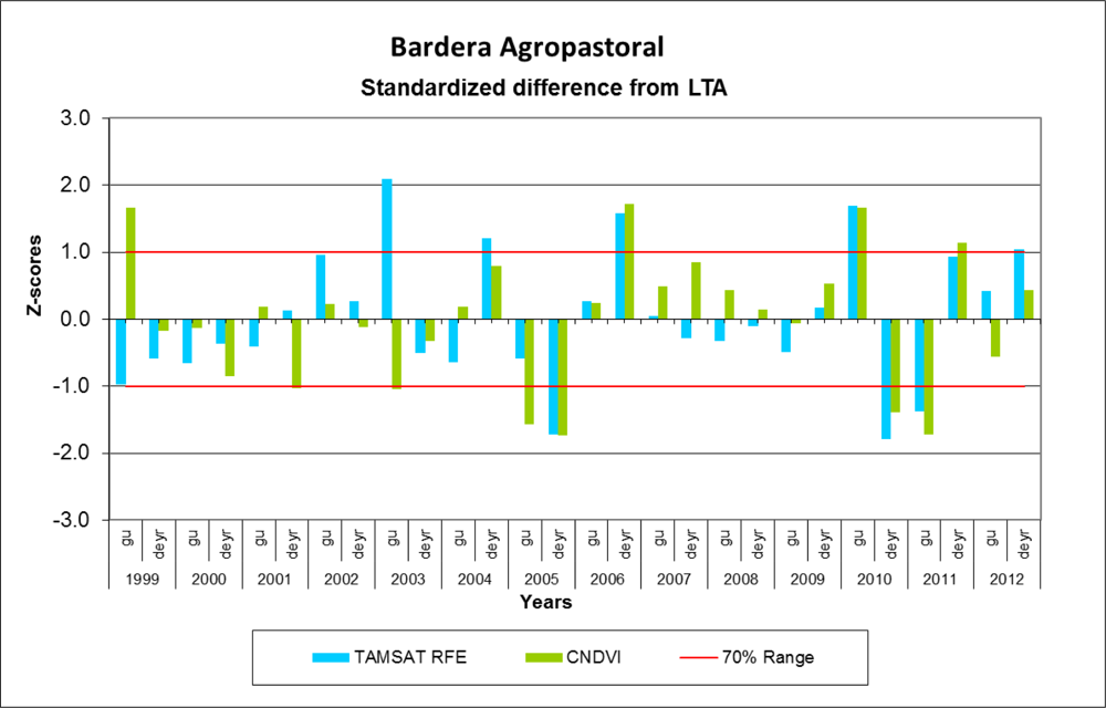
Finally, an effective way of analyzing the possible yield reduction due to variations in different commonly used yield proxies such as NDVI and rainfall, is the computation of z-scores of those variables cumulated over the crop season by using fixed start dates and season lengths [45]. At the end of the season this approach allows the rapid identification of positive or negative outliers as compared to the historical crop seasons and visualizes at the same time the relationship between different indicators. For example in the cases where NDVI and rainfall don’t show a deviation of the same sign and similar amplitude, other factors such as temporal rainfall distribution or change in crop areas must be taken into consideration (Figure 3).

3. Quantitative Crop Yield Predictions by Regression Modeling

In the previous section, approaches have been described using low resolution imagery for providing qualitative indications of crop growth (e.g., crop growth worse/better than average or start of the season earlier/later than average). In this section, two methods will be described that quantify the expected yield (e.g., in t/ha) using regression models. In contrast to the qualitative approaches, the regression approaches must necessarily be calibrated using appropriate reference information. In most cases, agricultural statistics and, specifically, crop yield are used as reference information. This pre-requisite limits its applicability in many regions of the world. We will distinguish purely remote sensing-based approaches (Section 3.1) and mixed approaches where additional bio-climatic predictor variables are used (Section 3.2). In both cases, appropriate crop masks are necessary. Only a few approaches were described not relying on independent crop masks. For example, Maselli and Rembold [46] used the regression between historical yields and cumulated NDVI at pixel level to derive fractions of agricultural area by pixel and restrict yield estimates to those fractions. Similarly, the yield-masking approach proposed by Kastens et al.[47] models crop yield at the administrative level through intelligent selection of appropriate proxy pixels. This approach is illustrated in more detail in Atzberger [1] and is therefore not covered in this review.

3.1. Use of Remotely Sensed Indicators for Crop Yield Prediction

The aforementioned relationship between vegetation indices and biomass/fAPAR enables the early estimation of crop yield, since yield of many crops is mainly determined by the photosynthetic activity of agricultural plants in certain periods prior to harvest [48,49]. In general, NDVI is used as an independent variable in empirical regression models to estimate final crop grain yield (the dependent variable). The basic assumption of this method is that sufficiently long and consistent time series of both remote sensing images and agricultural statistics are available. The latter are normally aggregated at the level of sub-national administrative units, for which average NDVI values can be extracted, either including or excluding a weighting of pixels according to crop coverage. An example of NDVI/yield regressions for cereals at national level is shown by Figure 4.
Many studies reported useful statistical relationships using NDVI values at the peak of the growing season and final crop yield once the perturbing effects of geographically variable environmental features (natural vegetation, soil types and conditions, topography, etc.) had been reduced. The different empirical techniques appear to be relatively accurate for crops with low final production because biomass is the limiting factor to yield and the relationship between the leaf area index (LAI) and the vegetation response (NDVI) is below the range of saturation [50]. Empirical relationships also appear to be relatively accurate for grass crops, where dry matter is the harvestable yield.
Linear regression models relating NDVI to crop yield have, for example, been developed by Rasmussen [51] and Groten [52] for Burkina Faso and by Maselli et al.[24] for Niger. The same and other investigations showed that yield forecasting can be obtained by the use of NDVI data of specific periods which depend on the eco-climatic conditions of the areas and the types of crop grown [5355].
It has to be noted that the correlation between crop yield and spectral measurements varies during the growing season, and regression coefficients show strong temporal variations [56,57]. Established relationships are therefore, to some degree, “good fortune” and rarely operational [48]. In cases where the above ground biomass is not the harvestable yield, one has also to consider that the relation between crop yield and spectral data is only indirect [53]. Besides classical (multiple) linear regression, other statistical techniques such as partial least square regression (PLSR) or principle component regression (PCR) may be more appropriate to model the relation between the sought variable and the spectral reflectances [58].
Various authors postulated that accumulated radiometric data are more closely related to crop production than instantaneous measurements. Several choices of temporal NDVI integration can be found, reaching from the simple selection of the maximum NDVI value of the season, to the average of the peak values (plateau) to the sum of the total NDVI values of the total crop cycle. An example for winter wheat yield estimation at national level is provided by Meroni et al.[59] for Tunisia. Instead of using a fixed integration period, the integral is computed between the start of the growing period and the beginning of the descending phase. The two dates are computed for each pixel and each crop season separately.
Pinter et al.[20] argued that the accumulation of radiometric data was similar to a measure of the duration of green leaf area. They consequently related yield of wheat and barley to an accumulated NDVI index and obtained satisfactory results. However, their results reveal that the performance of the integration is only optimum if it starts at a specific phenological event (i.e., at heading stage). When the optimum data could not be specified accurately, predictions were less accurate.
For the area of North America, Goward et al.[60] showed that an integrated NDVI from NOAA AVHRR gave a good description of the produced biomass. Tucker et al.[12] found a strong correlation between the integrated NOAA-7 NDVI data and end-of-season above-ground dry biomass for ground samples collected over a three-year period in the Sahel region. The correlation was higher than the one obtained from instantaneous NDVI values.
A third empirical technique involves the concept of aging or senescence, first developed by Idso et al.[61]. Idso and co-authors found that yield of wheat could be estimated by an evaluation of the rate of senescence as measured by a ratio index following heading. The lower the rate of senescence the larger the yield, as stressed plants begin to senesce sooner.
The same technique was later applied by Baret and Guyot [62]. They confirmed that final yield production in winter wheat was correlated with the senescence rate. However, the calculated regression coefficients of Baret and Guyot [62] were completely different from those of Idso et al.[61].
One important limitation of the yield/NDVI regression (as for any other empirical approach) is that most of the mentioned studies are linked to the environmental characteristics of specific geographic areas, or are limited by the availability of large and homogeneous datasets of low resolution data. A common problem in crop monitoring and yield forecasting in many countries of the world is the difficulty in extending locally calibrated forecasting methods to other areas or to other scales.
One should also note that where the crop area is not known, the NDVI/yield relationship does not provide information on final crop production, which is what many users of crop monitoring information are ultimately interested in. For this reason several authors have used NDVI to predict final crop production directly [25,53] or to estimate the fraction of NDVI inter-annual variability due to changes in crop area [55]. In general, a direct NDVI/production regression makes only sense under specific conditions, such as a stable crop area over the observed period. Otherwise, the reported statistics are purely artifacts.

3.2. Concomitant Use of Remotely Sensed Indicators Together with Bio-Climatic Indicators

In many cases, the predictive power of remotely sensed indicators can be improved by adding independent meteorological (or bio-climatic) variables into the regression models. Several bio-climatic and remote sensing-based indicators have proven to be highly correlated with yield for certain crops in specific areas [54,63,64]. These variables can be either measured directly (like rainfall coming from synoptic weather stations) or by satellites (like rainfall estimates) or can be the result of other models as it is normally the case of agro-meteorological variables like ETa (actual Evapo-transpiration) or soil moisture.
Potdar et al.[65] observed that the spatio-temporal rainfall distribution needs to be incorporated into crop yield models, in addition to vegetation indices deduced from remote sensing data, to predict crop yield of different cereal crops grown in rain-fed conditions. Such hybrid models show higher correlation and predictive capability than the models using remote sensing indicators only [66,67] as the input variables complement each other. The bio-climatic variables introduce information about solar radiation, temperature, air humidity and soil water availability while the spectral component introduces information about crop management, varieties and stresses not taken into consideration by the agro-meteorological models [57]. However, it must be noted that many bio-climatic indicators, especially if they are derived from satellites as well, are not really independent from vegetation indices. The interrelation of the different input variables should be considered and corrected when integrating bio-climatic and spectral indicators into multiple regression models.
Rasmussen used multiple regression models by introducing environmental information such as Tropical Livestock Unity (TLU or TLUDEN in Table 2) density and percentage of cultivated land [63] and arrived to explain 88% of the millet grain yield variance (Table 2).
Rojas [68] used the actual evapotranspiration (ETa) calculated by the FAO CWSB model and the CNDVI as independent variables in a regression analysis in order to estimate maize yield in Kenya during the first cropping season. CNDVI and ETa combined in the model to explain 83% of the maize crop yield variance with a root mean square error (RMSE) of 0.33 t/ha (coefficient of variation of 21%). The optimal prediction capability of the independent variables was 20 days and 30 days for the short and long maize crop cycles, respectively. If validated over long time series, such models are expected to be utilized in an operational way.
Although linear regression modeling is likely the most common method to produce yield predictions by using remote sensing-derived indicators together with bio-climatic information, this is not the only one. Numerous other methods have been developed that include, for instance, similarity analysis and neural networks [69].

4. Quantitative Yield Forecasts Using Crop Growth Models

The approaches for crop monitoring and yield predictions described in the two preceding sections were mainly based on profile comparison and regression models. In this section we will introduce a group of techniques involving modeling of crop physiology. According to the level of detail with which crop physiology is modeled, two approaches will be distinguished. The most sophisticated approach in this group of techniques is known as crop growth modeling, SVAT (Soil Vegetation Atmosphere) modeling or agro-meteorological modeling. This approach will be described in Section 4.2. Simplified approaches are mostly based on Monteith’s efficiency equation and are also known as NPP (Net primary production) models. This simpler approach will be treated in Section 4.1.
Crop growth modeling involves the use of mathematical simulation models including the analytical knowledge previously gained by plant physiologists [50]. The models describe the primary physiological mechanisms of crop growth (e.g., phenological development, photosynthesis, dry matter portioning and organogenesis), as well as their interactions with the underlying environmental driving variables (e.g., air temperature, soil moisture, nutrient availability) using mechanistic equations [50]. State variables (such as phenological development stage, biomass, leaf area index, soil water content, etc.) are updated in a computational loop that is usually performed daily [70]. This computational loop (and feedback) is not used in the simplified approach first described by Monteith in 1972 [71]. Instead, the total biomass production is assumed to equal the sum of the (daily) net primary production calculated in a simplified manner; one simply links the extent of active chlorophyllian surfaces with the duration of their activity and the incident photosynthetically active radiation to calculate biomass production. Both approaches have been successfully run with remotely sensed input and will be described in more detail in the following.

4.1. Estimation and Mapping of Absorbed Photosynthetically Active Radiation for Use in Monteith’s Efficiency Equation

The biomass production of a crop depends on the amount of photosynthetically active solar radiation (PAR) absorbed, as well as temperature conditions and water/nutrient availability. The amount of absorbed solar radiation depends on incoming radiation and the crop’s PAR interception capacity. The latter is mainly determined by crop leaf area and the incoming radiation can be provided by meteorological stations. The close relation between fAPAR and LAI explains why so many studies attempt to map leaf area (e.g., [70,72,73]).
Remotely sensed images were proposed in the 1980s for assessing and mapping of the crop’s assimilation potential. One of the first steps in this direction was the introduction of fAPAR in Monteith’s efficiency equation (1977) [73]. fAPAR is defined as the fraction of absorbed (APAR) to incident (PAR) photosynthetically active radiation (0 ≤ fAPAR ≤ 1):
fAPAR = APAR / PAR
fAPAR depends mainly (but not solely) on the leaf area of the canopy [74]. Generally, an exponential relation between leaf area index (LAI) and fAPAR is admitted:
fAPAR = fAPAR max ( 1 exp ( k × LAI ) )
with fAPARmax between 0.93 and 0.97 and extinction coefficient k between 0.6 and 2.2 [48].
Remotely sensed data can be used for mapping fAPAR as the latter is closely linked to canopy reflectance and NDVI[75]. The close link between NDVI and fAPAR has been confirmed both from theoretical considerations and experimental field studies. The studies agree that a linear relation between NDVI and fAPAR can be assumed:
fAPAR = a + b × NDVI
Most studies reviewed by Atzberger [56] found a slope (b) between 1.2 and 1.4 and an intercept (a) between −0.2 and −0.4. The negative intercept reflects the fact that the NDVI of bare soils (i.e., fAPAR = 0) is often between 0.2 and 0.4.
The relation between fAPAR and canopy reflectance/NDVI is not surprising because PAR interception and canopy reflectance/NDVI are functionally interdependent as they both depend on the same factors [48]. The main factors determining PAR interception and canopy reflectance/NDVI are—in order of decreasing importance—[56]: (i) leaf area index, (ii) leaf optical properties (especially leaf pigment concentration), (iii) leaf angle distribution, (iv) soil optical properties, and (v) sun zenith angle.
With the introduction of fAPAR, the mechanism by which the incident PAR is transformed into dry matter can be written as [75,76]):
Δ DM = PAR × fAPAR × ε b
with: ΔDM: net primary production (NPP) (g·m−2·d−1), PAR: incident photosynthetically active radiation (MJ·m−2·d−1), fAPAR: fraction of incident PAR which is intercepted and absorbed by the canopy (dimensionless), εb: light-use efficiency of absorbed photosynthetically active radiation (g·MJ−1)
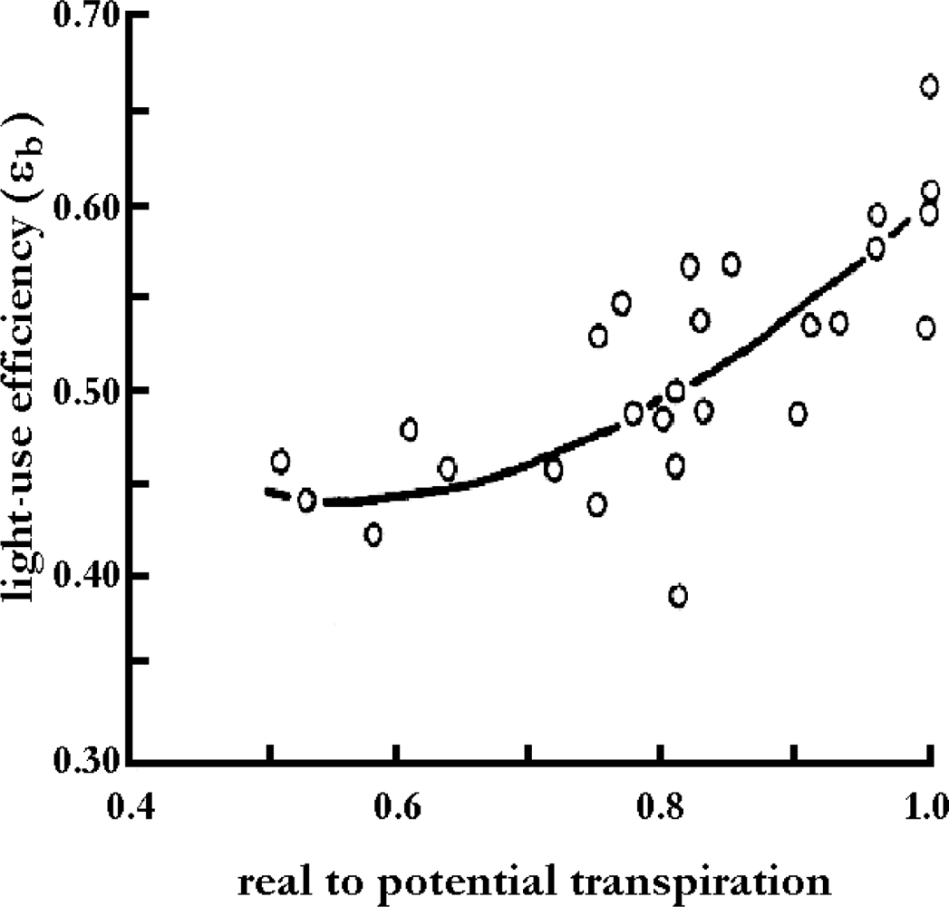
The light-use efficiency (εb) is relatively constant for crops like winter wheat (with a value of about 2.0 g·MJ−1) when calculated over the entire growth cycle and in the absence of growth stresses [48]. However, the light-use efficiency is not constant when calculated over small periods of the growth cycle. The short-term variability of the light-use efficiency is a result of temperature, nutrient and water conditions that eventually can lead to plant stress (Figure 5).
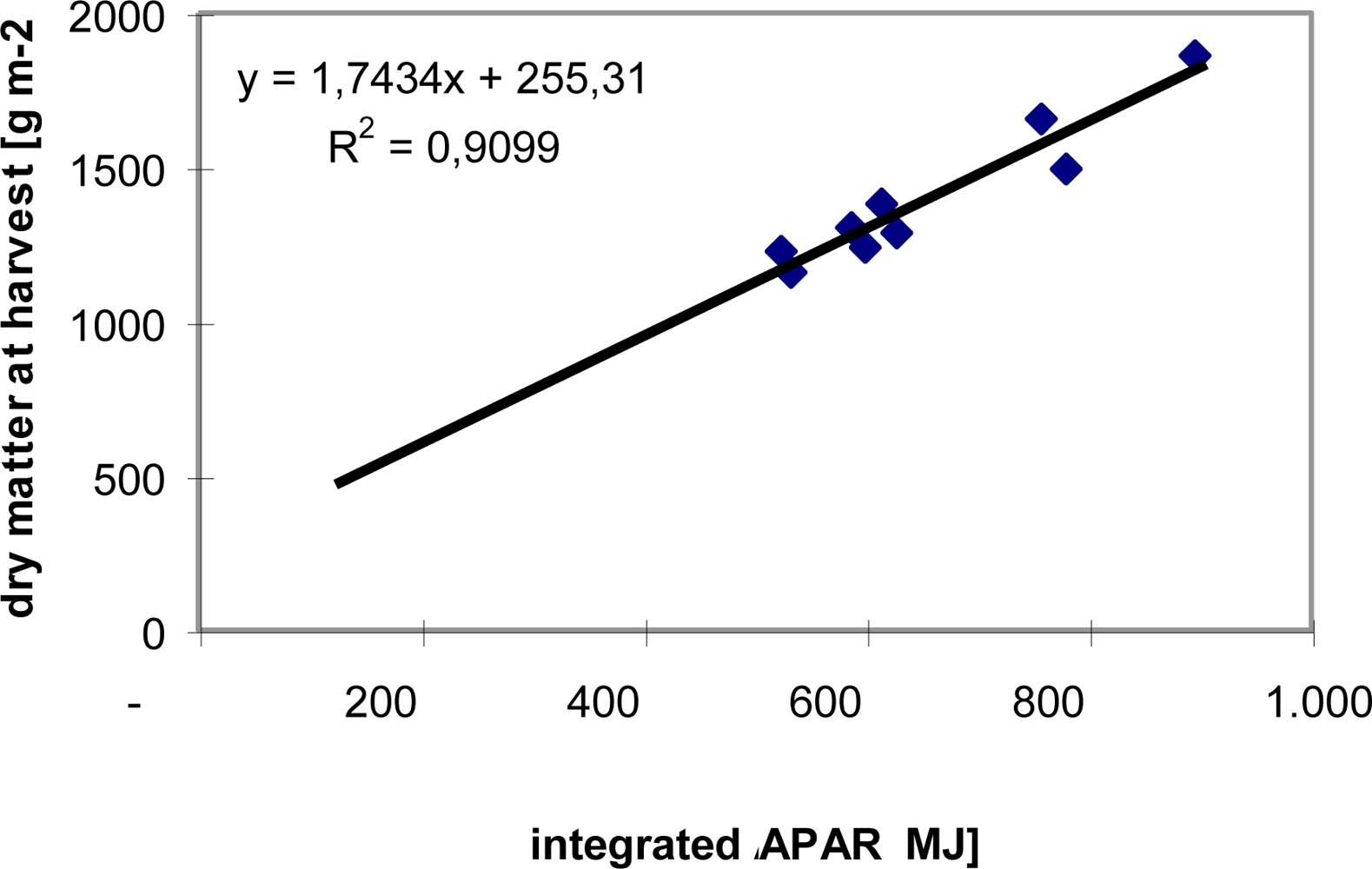
Remotely sensed data can be used in Monteith’s efficiency equation (Equation (5)) if one manages to map the seasonal cycle of fAPAR (if enough images are available so that the full temporal profile can be reconstructed). As explained, at the same time, the light-use efficiency (εb) must either be relatively constant/known or should be assessed using other remote sensing inputs (e.g., from thermal data). Provided that enough images are available, the seasonal integration of radiometric measurements theoretically improves the capability of estimating biomass compared to one-time measurements, since the approach is based on sound physical and biological theory, whereas the relationship between instantaneous measurements of canopy reflectance and biomass is mainly empirical, and, to some degree, chance [48]. For example, Figure 6 shows the close correspondence between seasonally integrated absorbed PAR (fAPAR × PAR) and the dry matter at harvest for nine commercial winter wheat plots in the Camargue region of France ([56]. Note that the slope (here 1, 7) in Figure 6 corresponds to εb in Equation (5).
Nowadays, fAPAR is routinely assessed using various approaches and algorithms (for example, see [78,79]) and applied to different sensors (VEGETATION, MODIS, AVHRR and others). Likewise, operational NPP products based on Monteith’s formula are available (e.g., from MODIS).
Monteith’s efficiency equation has been further extended to include, for example, temperature dependency of photosynthesis and respiration. For example, VITO [80] uses the following formula for the NPP calculation:
Δ DM = PAR × fAPAR × ε b × p ( T ) × CO 2 fert × ( 1 r ( T ) )
  • where: ΔDM: increase in dry matter (DM) or net primary production (NPP) (g·m−2·d−1)
  • PAR: incident photosynthetically active solar radiation (MJ·m−2·d−1)
  • fAPAR: Fraction of intercepted and absorbed PAR; fAPAR is estimated from the remotely sensed NDVI by means of a linear equation, suggested by Myneni and Williams [81] (dimensionless)
  • εb: Photosynthetic efficiency, [82] (g·MJ−1)
  • p(T): Normalized temperature dependency factor as defined by Johnson et al.[83], and parameterized according to data of Lommen et al.[84] (dimensionless)
  • CO2fert: Normalized CO2 fertilization factor, [85] (dimensionless)
  • r(T): fraction of assimilated photosynthesis consumed by autotrophic respiration; r is modeled as a simple linear function of daily mean air temperature, [60].
Hence, compared to Equation (5), εb is reduced/increased as a function of temperature and CO2 content to mimic the above mentioned plant reactions to changing growth conditions.
In either case, to calculate final yield (Y) in the framework of Monteith’s efficiency equation, it has to be assumed that a portion of the cumulated biomass at the end of the growing season (the harvest index, HI) is the harvestable yield, i.e.,
Y = HI × sowing harvest Δ DM
The harvest index (HI) may be obtained by traditional regression analysis between primary production and statistical crop yields. According to the MARS project, for instance, the use of cumulated dry matter over the crop growing period gives more reliable results compared with NDVI for crop yield forecasting in many Mediterranean and Central Asian countries [86]. For corn, Gallo et al.[87] found that the cumulated daily absorbed PAR computed with fAPAR predicted from NDVI, and that the daily incident PAR explained 73 percent of the variance in the observed grain yield. Only 56 and 58 percent of variance were accounted by the cumulated LAI and cumulated NDVI, respectively.
The main disadvantage of models based on Monteith’s efficiency equation is the same as for the approaches described in Section 3.1; i.e., the spatial resolution of low resolution remote sensing data is often too coarse to resolve, for example, individual fields. As a result, the fAPAR values represent the average photosynthetic activity of all vegetation inside the pixel. However, the share of the crop fraction in common greenness can be highly variable from pixel to pixel. Thus, the calculated ΔDM values characterize the vegetation status in general without relating to concrete crop (except that exceptional cases with pixels are completely covered by a single crop).

4.2. Parameterization and Re-Calibration of Crop Growth Models

Crop growth models describe the primary physiological mechanisms of crop growth and development in a computational loop (Figure 7). Model state variables such as development stage, organ dry mass and leaf area index (LAI) are linked to environmental driving variables such as temperature and precipitation, which are usually provided with a daily time step [50]. Soil and plant parameters are used to mimic the plant’s reaction to these driving variables. Whereas model state variables are updated within the computational loop, model parameters remain unchanged during the simulation run (e.g., soil texture information). All state variables should be initialized at the beginning of the simulation run.
Simulation models are excellent analytical tools because they exhibit three distinct characteristics that distinguish them from the previously described approaches [50]:
  • they are dynamic, in that they operate on a time step for ordering input data and updating state variables
  • they contain parameters that allow a general scheme of equations to be adopted to the specific growth behavior of different crop species
  • they include a strategy for describing phenological development of a crop to order organ appearance and assimilate portioning.
The first crop simulation models were developed by the end of World War II [88]. In subsequent decades, they became both more complex and potentially more useful [89]. Deterministic crop growth models have been validated for cereals, as well as for potato, sugar beet, oilseed, rice, canola and sunflower. Most of these models include water and energy balance modules and run on a daily basis over the whole life cycle of a crop. Prominent models are, for example, CERES [90], WOFOST [91], OILCROPSUN [92], CROPSYST [93] and STICS [94]. Some simpler models (without water and energy balance) such as GRAMI [95,96] also exist. More sophisticated models attempt to integrate numerous factors that affect crop growth and development, such as plant available soil water, temperature, wind, genetics, management choices, and pest infestations. Currently, attempts are made to permit the integration and combination of various sub-models from different model developers describing a specific plant behavior (e.g., phenology) [97]. The strength of these models as research tools resides in their ability to capture the soil-environment-plant interactions, but their initialization and parameterization generally requires a number of physiological and pedological parameters that are not easily acquired. Careful validation strategies have to be employed for obtaining meaningful results [98].
Crop growth models and remote sensing complement one another since crop growth models provide a continuous estimate of crop growth over time, whilst remote sensing provides spatial pictures of crop status (e.g., LAI) within a given area [28,76,99,100]. The complementary nature of remote sensing and crop growth modeling was first recognized by S. Maas from USDA who described routines for using satellite-derived information in mechanistic crop models. Remotely sensed images are particularly useful in spatially distributed modeling attempts [101,102]. In spatially distributed modeling all model inputs and parameters have to be provided in spatialized form. As remote sensing provides spatial status maps, the use of remotely sensed information makes the crop growth models more robust [102,103].
Spatialized information is readily available concerning many meteorological driving variables (e.g., from global circulation models like ECMWF). In an operational yield estimation program, however, it might not be feasible to obtain the necessary pixel by pixel on-site: (i) soil, plant and management parameters, and (ii) initial values of all crop state variables required by sophisticated crop growth models. In the reminder of this sub-section, we present different approaches for using remote sensing data in spatially distributed crop growth modeling. The ideas are extracted from the outstanding paper of Delecolle et al.[50]. Note that the albeit important provision of meteorological driving variables by satellite imagery will not be considered because a description of the meteorological remote sensing would be too lengthy. Interested readers may, for example, refer to Thornton et al.[104].
In the most straightforward way, remote sensing may be used to parameterize and/or initialize crop growth models. In the context of this review, the term “parameterization” refers to the provision of model parameters required by crop growth and agro-meteorological models, e.g., soil texture information, photosynthetic pathway information, crop type, sowing date, etc. The term “initialization” refers to the provision of model state variables at the start of the simulation. Note that all state variables need to be initialized. In some cases, this initialization is simple and straightforward. For example, it is reasonable to assume the initial value of LAI at sowing to be zero. However, the soil water content at sowing may be highly variable. For the purpose of parameterization or initialization, satellite imagery covering different wavelength ranges (i.e., optical to microwave) may be combined [105]. In the simplest case, remotely sensed data is used to provide information about crop type [106]. With known crop types, plant specific parameter settings can be assigned (therefore the term parameterization). Optical imagery of bare soil conditions may be used to map soil organic matter content, soil texture and soil albedo [107110]. These three model parameters are often used in crop growth models as they influence nutrient release, water capacity and radiation budget [111]. Other imagery (e.g., microwave) may be used to provide an estimate of soil water content at the beginning of the simulation run, i.e., at sowing [112]. This will be called model initialization, as the state variable “soil water content” has been attributed a value for the start of the simulation.
Besides the direct parameterization and initialization of crop growth models, remote sensing can be used at least in four other valuable ways:
  • Re-calibration or re-parameterization
  • Re-initialization
  • Forcing
  • Updating
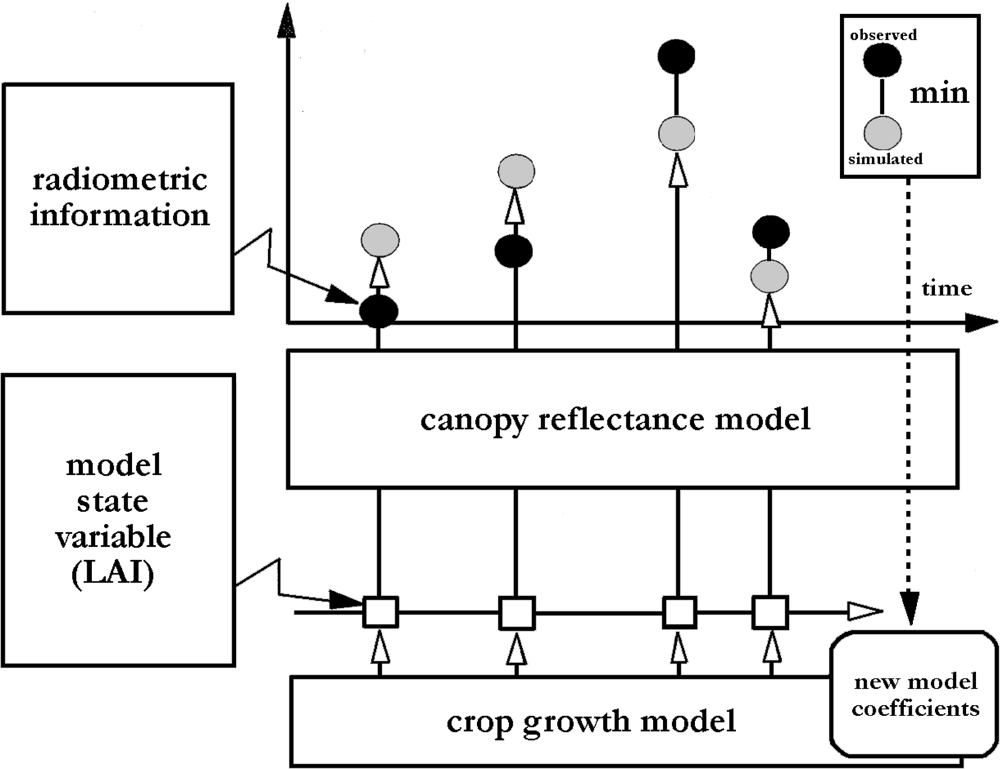
In the “re-calibration” or “re-parameterization” approach, one assumes that some parameters of the crop growth model are inaccurately calibrated, although the model as a whole is formally adequate [50]. By providing reference observations (e.g., LAI) for the times that they are available, some crop model parameters can be calibrated (Figure 8). This is usually achieved by (iteratively) adjusting the model parameters until measured and simulated profiles of the state variables (here: reflectance values) match each other. In spatially distributed modeling this re-calibration has of course to be done pixel by pixel.
The “re-initialization” of crop growth models works in a very similar way; however, instead of adjusting model parameters, one simply tunes the initial values of state variables until a good match between observed and simulated state variables is obtained. In both cases, the remote sensing derived state variables are considered as an absolute reference for the model simulation. The exact timing of the remotely sensed observations is of minor importance. Already as few as one reference observation is useful [56]. However, the more satellite observations are available and the better they are distributed across the growing season, the more/better model parameters can be calibrated and/or initialized.
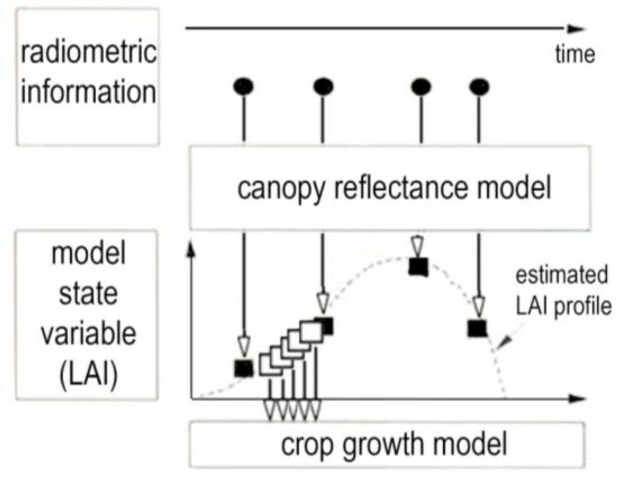
Alternatively, one may also choose to infer important state variables from remotely sensed data for each time step of the model simulation (e.g., LAI) for direct ingestion into the model, thus “forcing” the model to follow the remotely sensed information (Figure 9). Such a simplification makes crop growth models very similar to the Monteith efficiency equation (Section 4.1), as one breaks the computational loop in the model shown in Figure 7. As the model does no longer determine the values of that variable by itself, inconsistent model states may result.
In a very similar way, remotely sensed data are used in the “updating” of crop growth models. One simply replaces simulated values of crop state variables by remotely sensed values each time these are available (not necessarily at each time step). The computations then continue with these updated values until new (remote sensing) inputs are provided. As for the “forcing” method, the replacement of simulated by observed state variables may result in inconsistent model states as one does not correct for apparent errors in the model calibration, which are causing the differences between simulated and observed state variables.

5. Conclusions

The large number of existing studies proves the relevance of low resolution satellite images for crop monitoring and yield prediction at the regional level and under different environmental circumstances. The relatively limited costs generally associated with the acquisition of low resolution satellite images makes them an attractive instrument for crop monitoring and yield forecasting. Government institutions have in many countries developed operational systems using one or more of the methodologies described in this review together with ground data. In the United States, the USDA (United States Department of Agriculture) FAS (Foreign Agriculture Service) makes extensive use of remote sensing for the assessment of world agriculture with an approach based more on human expertise [113] than on highly automatic systems. At the national level, the NASS (National Agricultural Statistics Service) is using remote sensing as auxiliary information for integrating and improving the precision of their statistical sampling methods for crop acreage and crop yield estimates [114]. In Europe, the MARS project was launched more than 20 years ago with the main objective of providing early yield and area estimates all over Europe based on remote sensing techniques [115]. For semiarid to arid countries, numerous pre-operational systems for yield forecasts at an early stage of the growing season have been proposed. Most of them are based on low resolution satellite imagery and combine the NDVI with several bio-climatic indicators reaching from rainfall to tropical livestock density [63,116]. The USAID-funded FEWSNET (Famine Early Warning Systems Network) regularly issues food security reports and outlooks for the most food insecure countries around the world largely based on the use of medium resolution satellite images and their integration with ground data [117].
With the renewed focus on agricultural production following the 2008 food crisis, yield forecasting based on low resolution remote sensing continues to be seen as a relevant tool for global crop monitoring as demonstrated by a series of global and regional initiatives such as the G20 initiatives GEO-Global Agricultural Monitoring (GEO-GLAM) and the Agricultural Markets Information System (AMIS), as well as the strengthening or geographic extension of existing monitoring systems such as GLOBECAST (former Agri4cast in MARS) and FEWSNET (30 new countries covered by remote monitoring).
The methodological evolution will have to lead this expansion, not only by exploiting satellite images that are becoming available with new sensors (e.g., SENTINEL), but also by continuing to improve the integration between satellite data and crop growth models. More variables derived from satellite images which are closely related to crop yield will further improve yield forecasts, as is happening, for example, with the Actual Evapotranspiration derived from the thermal information of sensors such as Meteosat and MODIS and global meteorological data [118,119]. Improvements in model validation can be expected from innovative approaches of farm data collection such as the crowdsourcing approaches experimented by Fritz et al.[120].
It should not be forgotten, however, that the intrinsic limitations of low resolution images cannot be totally overcome even by sophisticated methodologies. Most of the mentioned operational systems use low resolution satellite images mainly to support ground assessments or as a proxy for yield forecasts used in combination with other important factors, such as the historical trend or crop growth model outputs. Concerning yield forecasts based both on regression estimates and models, positive results in study areas limited in space are not sufficient to encourage the inclusion of the described methods in large operational systems.
Probably the most serious limitation for most of the quantitative methods described in this chapter remains the availability, but also the aggregation level of, publicly accessible agricultural statistics like crop yield or area. In fact, during agricultural surveys, these statistics are usually measured at field level and their extension and aggregation to larger administrative areas requires an intense surveying effort. For analysis with low resolution satellite images, agricultural statistics are generally needed at a highly aggregated level like districts or provinces. In many countries of the world, the availability of such data is extremely reduced and, if existent, they are not always easily accessible, or highly reliable. Also, once the data have been aggregated, it is extremely difficult to verify their accuracy.
Eventually, as with any satellite images, no analysis should be done without good ground truth data, and the final results remain heavily dependent on the quality of the ground data. Low resolution remote sensing images should never be seen as a way to replace these data, but more as a combination of different techniques in order to reduce the three strongest limitations of ground observations: high cost, lack of timeliness, and insufficient spatial coverage.
In general, technical progress in science and industry leads to a trend in remote sensing towards higher resolution which parallels the larger availability of powerful data processing devices on the user’s side. Although a general link exists between an increase in resolution and the quality of crop monitoring information and yield forecasts, the relationship is not strictly linear. It is therefore extremely difficult to evaluate the exact benefit of each gain of resolution for crop monitoring and yield forecasting. Spatial patterns in agriculture, such as field size, play a fundamental role in defining what is the best resolution for a certain region. Significant improvements in monitoring yield, but especially for crop acreage, can be expected when the area corresponding to one pixel becomes several times smaller than the field size. In this way, the mixed pixel problem is significantly reduced, since most pixels can be assumed to “match” with real fields. The extreme consequence of this is that areas with highly fragmented agricultural patterns, as many rural zones in Europe, and most of the traditional African agriculture, will remain difficult areas to monitor unless pixel size goes clearly below one hectare.
Finally, despite the positive continuous trend in increasing spatial resolution, the length of the available time series also plays an important role in the yield forecasting methods described. Most of the methods described are based on the use of long time series for comparison with previous years or with the average situation and those methods cannot profit immediately from the availability of higher spatial resolution sensors. This means that even when the next generation of earth-observing satellites with higher spatial ground sampling distance will be launched (e.g., Sentinel-2 and Proba-V to be launched end of 2014), a number of years will pass until the benefits of the increased spatial resolution will have their full impact on improving the quality of yield forecasts. Increased research efforts on sensor inter-calibration are needed to simplify access to long time series of remotely sensed data from different sensors.

References

  1. Atzberger, C. Advances in remote sensing of agriculture: Context description, existing operational monitoring systems and major information needs. Remote Sens 2013, 5, 949–981. [Google Scholar]
  2. Johnson, G.E.; van Dijk, A.; Sakamoto, C.M. The use of AVHRR data in operational agricultural assessment in Africa. Geocarto. Int 1987, 2, 41–60. [Google Scholar]
  3. Hutchinson, C.F. Uses of satellite data for famine early warning in Sub-Saharan Africa. Int. J. Remote Sens 1991, 12, 1405–1421. [Google Scholar]
  4. Busetto, L.; Meroni, M.; Colombo, R. Combining medium and coarse spatial resolution satellite data to improve the estimation of sub-pixel NDVI time series. Remote Sens. Environ 2008, 112, 118–131. [Google Scholar]
  5. Atkinson, P.M.; Cutler, M.E.J.; Lewis, H. Mapping sub-pixel proportional land cover with AVHRR imagery. Int. J. Remote Sens 1997, 18, 917–935. [Google Scholar]
  6. Foody, G.M.; Cox, D.P. Sub-pixel land cover composition estimation using a linear mixture model and fuzzy membership functions. Int. J. Remote Sens 1994, 15, 619–631. [Google Scholar]
  7. Atzberger, C.; Rembold, F. Mapping the spatial distribution of winter crops at sub-pixel level using AVHRR NDVI time series and neural nets. Remote Sens 2013, 5, 1335–1354. [Google Scholar]
  8. Tucker, C.J. Red and photographic infrared linear combinations for monitoring vegetation. Remote Sens. Environ 1979, 8, 127–150. [Google Scholar]
  9. Tucker, C.J.; Holben, B.N.; Elgin, J.H., Jr.; McMurtrey, J.E., III. Relationship of spectral data to grain yield variation. Photogramm. Eng. Remote Sensing 1980, 46, 657–666. [Google Scholar]
  10. Deering, D.W. Rangeland Reflectance Characteristics Measured by Aircraft and Spacecraft Sensors. 1978. [Google Scholar]
  11. Macdonald, R.B.; Hall, F.G. Global crop forecasting. Science 1980, 208, 670–679. [Google Scholar]
  12. Tucker, C.J.; Vanpraet, C.; Boerwinkel, E.; Gaston, A. Satellite remote sensing of total dry matter production in the Senegalese Sahel. Remote Sens. Environ 1983, 13, 461–474. [Google Scholar]
  13. Sellers, P.J. Canopy reflectance, photosynthesis and transpiration. Int. J. Remote Sens 1985, 6, 1335–1372. [Google Scholar]
  14. Prince, S.D. High Temporal Frequency Remote Sensing of Primary Production Using NOAA AVHRR. In Applications of Remote Sensing in Agriculture; Steven, M.D., Clark, J.A., Eds.; Butterworths: London, UK, 1990; pp. 169–183. [Google Scholar]
  15. Los, S.O. Linkages between Global Vegetation and Climate: An Analysis based on NOAA Advanced Very High Resolution Data. 1998. [Google Scholar]
  16. Tucker, C.J.; Holben, B.N.; Elgin, J.H., Jr.; McMurtrey, J.E., III. Remote sensing of total dry-matter accumulation in winter wheat. Remote Sens. Environ 1981, 11, 171–189. [Google Scholar]
  17. Tucker, C.J.; Sellers, P.J. Satellite remote sensing of primary production. Int. J. Remote Sens 1986, 7, 1395–1416. [Google Scholar]
  18. Running, S.W.; Nemani, R.R. Relating seasonal patterns of the AVHRR vegetation index to simulated photosynthesis and transpiration of forests in different climates. Remote Sens. Environ 1988, 24, 347–367. [Google Scholar]
  19. Prince, S.D. Satellite remote sensing of primary production: Comparison of results for Sahelian grasslands 1981–1988. Int. J. Remote Sens 1991, 12, 1301–1311. [Google Scholar]
  20. Pinter, P.J., Jr.; Jackson, R.D.; Idso, S.B.; Reginato, R.J. Multidate spectral reflectance as predictors of yield in water stressed wheat and barley. Int. J. Remote Sens 1981, 2, 43–48. [Google Scholar]
  21. Barnett, T.L.; Thompson, D.R. Large-area relation of Landsat MSS and NOAA-6 AVHRR spectral data to wheat yields. Remote Sens. Environ 1983, 13, 277–290. [Google Scholar]
  22. Quarmby, N.A.; Milnes, M.; Hindle, T.L.; Silleos, N. The use of multi-temporal NDVI measurements from AVHRR data for crop yield estimation and prediction. Int. J. Remote Sens 1993, 14, 199–210. [Google Scholar]
  23. Henricksen, B.L.; Durkin, J.W. Growing period and drought early warning in Africa using satellite data. Int. J. Remote Sens 1986, 7, 1583–1608. [Google Scholar]
  24. Maselli, F.; Conese, C.; Petkov, L.; Gilabert, M.A. Environmental monitoring and crop forecasting in the Sahel through the use of NOAA NDVI data. A case study: Niger 1986–89. Int. J. Remote Sens 1993, 14, 3471–3487. [Google Scholar]
  25. Rao, C.R.N.; Chen, J. Revised post-launch calibration of the visible and near-infrared channels of the Advanced Very High Resolution Radiometer (AVHRR) on the NOAA-14 spacecraft. Int. J. Remote Sens 1999, 20, 3485–3491. [Google Scholar]
  26. Meygret, A.; Briottet, X.; Henry, P.; Hagolle, O. Calibration of SPOT4 HRVIR and VEGETATION cameras over the Rayleigh scattering. Proc. SPIE 2000, 4135, 302–313. [Google Scholar]
  27. Yin, H.; Udelhoven, T.; Fensholt, R.; Pflugmacher, D.; Hostert, P. How NDVI trends from AVHRR and SPOT VGT time series differ in agricultural areas: An Inner Mongolian case study. Remote Sens 2012, 4, 3364–3389. [Google Scholar]
  28. Meroni, M.; Atzberger, C.; Vancutsem, C.; Gobron, N.; Baret, F.; Lacaze, R.; Eerens, H.; Leo, O. Evaluation of agreement between space remote sensing SPOT-VEGETATION fAPAR time series. IEEE Trans. Geosci. Remote Sens 2012, 51, 1–12. [Google Scholar]
  29. Hird, J.N.; McDermid, G.J. Noise reduction of NDVI time series: An empirical comparison of selected techniques. Remote Sens. Environ 2009, 113, 248–258. [Google Scholar]
  30. Holben, B.N. Characteristics of maximum-value composite images from temporal AVHRR data. Int. J. Remote Sens 1986, 7, 1417–1434. [Google Scholar]
  31. Atzberger, C.; Eilers, P.H.C. Evaluating the effectiveness of smoothing algorithms in the absence of ground reference measurements. Int. J. Remote Sens 2011, 32, 3689–3709. [Google Scholar]
  32. Genovese, G.; Vignolles, C.; Nègre, T.; Passera, G. A methodology for a combined use of normalised difference vegetation index and CORINE land cover data for crop yield monitoring and forecasting. A case study on Spain. Agronomie 2001, 21, 91–111. [Google Scholar]
  33. Kerdiles, H.; Grondona, M.O. NOAA-AVHRR NDVI decomposition and subpixel classification using linear mixing in the Argentinean Pampa. Int. J. Remote Sens 1995, 16, 1303–1325. [Google Scholar]
  34. Kogan, F.N. Droughts of the late 1980s in the United States as derived from NOAA polar orbiting satellite data. Bull. Amer. Meteor. Soc 1995, 76, 655–668. [Google Scholar]
  35. Kogan, F.N. Operational space technology for global vegetation assessment. Bull. Amer. Meteor. Soc 2001, 89, 1949–1964. [Google Scholar]
  36. Rojas, O.; Vrieling, A.; Rembold, F. Assessing drought probability for agricultural areas in Africa with coarse resolution remote sensing imagery. Remote Sens. Environ 2011, 115, 343–352. [Google Scholar]
  37. Balint, Z.; Mutua, F.M. Drought Monitoring with the Combined Drought Index; FAO-SWALIM: Nairobi, Kenya, 2011; p. 32. [Google Scholar]
  38. Reed, B.C.; White, M.; Brown, J.F. Remote Sensing Phenology. In Phenology: An Integrative Environmental Science; Schwartz, M.D., Ed.; Kluwer Academic Publishers: New York, NY, USA, 2003; pp. 365–382. [Google Scholar]
  39. White, M.A.; de Beurs, K.M.; Didan, K.; Inouye, D.W.; Richardson, A.D.; Jensen, O.P.; O’Keefe, J.; Zhang, G.; Nemani, R.R.; van Leeuwen, W.J.D.; et al. Intercomparison, interpretation, and assessment of spring phenology in North America estimated from remote sensing for 1982–2006. Glob. Chang. Biol 2009, 15, 2335–2359. [Google Scholar]
  40. Zhang, X.; Friedl, M.A.; Schaaf, C.B.; Strahler, A.H.; Hodges, J.C.F.; Gao, F.; Reed, B.C.; Huete, A. Monitoring vegetation phenology using MODIS. Remote Sens. Environ 2003, 84, 471–475. [Google Scholar]
  41. Beck, P.S.A.; Atzberger, C.; Høgda, K.A.; Johansen, B.; Skidmore, A.K. Improved monitoring of vegetation dynamics at very high latitudes: A new method using MODIS NDVI. Remote Sens. Environ 2006, 100, 321–334. [Google Scholar]
  42. Atzberger, C.; Eilers, P.H.C. A time series for monitoring vegetation activity and phenology at 10-daily time steps covering large parts of South America. Int. J. Appl. Earth Obs. Geoinf 2011, 4, 365–386. [Google Scholar]
  43. Vrieling, A.; de Beurs, K.M.; Brown, M.E. Variability of African farming systems from phenological analysis of NDVI time series. Clim. Chang 2011, 109, 455–477. [Google Scholar]
  44. Atkinson, P.M.; Jeganathan, C.; Dash, J.; Atzberger, C. Inter-comparison of four models for smoothing satellite sensor time-series data to estimate vegetation phenology. Remote Sens. Environ 2012, 123, 400–417. [Google Scholar]
  45. Food Security and Nutrition Analysis Post Deyr 2012/13; Technical Series Report No VI. 50; Food Security and Nutrition Analysis Unit: Nairobi, Kenya, 2013; p. 174.
  46. Maselli, F.; Rembold, F. Analysis of GAC NDVI data for cropland identification and yield forecasting in Mediterranean African countries. Photogramm. Eng. Remote Sensing 2001, 67, 593–602. [Google Scholar]
  47. Kastens, J.H.; Kastens, T.L.; Kastens, D.L.A.; Price, K.P.; Martinko, E.A.; Lee, R.-Y. Image masking for crop yield forecasting using AVHRR NDVI time series imagery. Remote Sens. Environ 2005, 99, 341–356. [Google Scholar]
  48. Baret, F.; Guyot, G.; Major, D.J. Crop biomass evaluation using radiometric measurements. Photogrammetria 1989, 43, 241–256. [Google Scholar]
  49. Benedetti, R.; Rossini, P. On the use of NDVI profiles as a tool for agricultural statistics: The case study of wheat yield estimate and forecast in Emilia Romagna. Remote Sens. Environ 1993, 45, 311–326. [Google Scholar]
  50. Delécolle, R.; Maas, S.J.; Guérif, M.; Baret, F. Remote sensing and crop production models: Present trends. ISPRS J. Photogramm 1992, 47, 145–161. [Google Scholar]
  51. Rasmussen, M.S. Assessment of millet yields and production in northern Burkina Faso using integrated NDVI from the AVHRR. Int. J. Remote Sens 1992, 13, 3431–3442. [Google Scholar]
  52. Groten, S.M.E. NDVI-crop monitoring and early yield assessment of Burkina Faso. Int. J. Remote Sens 1993, 14, 1495–1515. [Google Scholar]
  53. Hayes, M.J.; Decker, W.L. Using NOAA AVHRR data to estimate maize production in the United States Corn Belt. Int. J. Remote Sens 1996, 17, 3189–3200. [Google Scholar]
  54. Lewis, J.E.; Rowland, J.; Nadeau, A. Estimating maize production in Kenya using NDVI: Some statistical considerations. Int. J. Remote Sens 1998, 19, 2609–2617. [Google Scholar]
  55. Maselli, F.; Romanelli, S.; Bottai, L.; Maracchi, G. Processing of GAC NDVI data for yield forecasting in the Sahelian region. Int. J. Remote Sens 2000, 21, 3509–3523. [Google Scholar]
  56. Atzberger, C. Estimates of Winter Wheat Production through Remote Sensing and Crop Growth Modelling: A Case Study on the Camargue Region. 1997. [Google Scholar]
  57. Rudorff, B.F.T.; Batista, G.T. Spectral response of wheat and its relationship to agronomic variables in the tropical region. Remote Sens. Environ 1990, 31, 53–63. [Google Scholar]
  58. Atzberger, C.; Guerif, M.; Baret, F.; Werner, W. Comparative analysis of three chemometric techniques for the spectroradiometric assessment of canopy chlorophyll content in winter wheat. Comput. Electron. Agric 2010, 73, 165–173. [Google Scholar]
  59. Meroni, M.; Marinho, E.; Sghaier, N.; Verstrate, M.M.; Leo, O. Remote sensing based yield estimation in a stochastic framework—Case study of durum wheat in Tunisia. Remote Sens 2013, 5, 539–557. [Google Scholar]
  60. Goward, S.N.; Dye, D.G. Evaluating North American net primary productivity with satellite observations. Adv. Space Res 1987, 7, 165–174. [Google Scholar]
  61. Idso, S.B.; Pinter, P.J., Jr.; Jackson, R.D.; Reginato, R.J. Estimation of grain yields by remote sensing of crop senescence rates. Remote Sens. Environ 1980, 9, 87–91. [Google Scholar]
  62. Baret, F.; Guyot, G. Monitoring of the ripening period of wheat canopies using visible and near infra red radiometry [reflectance, vegetation index, senescence rate, water plateau]. Agronomie 1986, 6, 509–516. [Google Scholar]
  63. Rasmussen, M.S. Developing simple, operational, consistent NDVI-vegetation models by applying environmental and climatic information. Part II: Crop yield assessment. Int. J. Remote Sens 1998, 19, 119–139. [Google Scholar]
  64. Reynolds, C.A.; Yitayew, M.; Slack, D.C.; Hutchinson, C.F.; Huetes, A.; Petersen, M.S. Estimating crop yields and production by integrating the FAO Crop Specific Water Balance model with real-time satellite data and ground-based ancillary data. Int. J. Remote Sens 2000, 21, 3487–3508. [Google Scholar]
  65. Potdar, M.B.; Manjunath, K.R.; Purohit, N.L. Multi-season atmospheric normalization of NOAA AVHRR derived NDVI for crop yield modeling. Geocarto. Int 1999, 14, 51–56. [Google Scholar]
  66. Manjunath, K.R.; Potdar, M.B.; Purohit, N.L. Large area operational wheat yield model development and validation based on spectral and meteorological data. Int. J. Remote Sens 2002, 23, 3023–3038. [Google Scholar]
  67. Balaghi, R.; Tychon, B.; Eerens, H.; Jlibene, M. Empirical regression models using NDVI, rainfall and temperature data for the early prediction of wheat grain yields in Morocco. Int. J. Appl. Earth Obs. Geoinf 2008, 10, 438–452. [Google Scholar]
  68. Rojas, O. Operational maize yield model development and validation based on remote sensing and agro-meteorological data in Kenya. Int. J. Remote Sens 2007, 28, 3775–3793. [Google Scholar]
  69. Stathakis, D.; Savin, I.Y.; Nègre, T. Neuro-Fuzzy Modeling for Crop Yield Prediction. Proceedings of the ISPRS Commission VII Symposium Remote Sensing: From Pixels to Processes, Enschede, The Netherlands, 8–11 May 2006.
  70. Guérif, M.; Delécolle, R. Introducing Remotely Sensed Estimates of Canopy Structure into Plant Models. In Canopy Structure and Light Microclimate. Characterization and Applications; Varlet-Grancher, C., Bonhomme, R., Sinoquet, H., Eds.; INRA: Paris, France, 1993; pp. 479–490. [Google Scholar]
  71. Monteith, J.L. Solar radiation and productivity in tropical ecosystems. J. Appl. Ecol 1972, 9, 747–766. [Google Scholar]
  72. Vuolo, F.; Neugebauer, N.; Falanga, S.; Atzberger, C.; D’Urso, G. Estimation of Leaf Area Index using DEIMOS-1 data: Calibration and transferability of a semi-empirical relationship between two agricultural areas. Remote Sens 2013, 5, 1274–1291. [Google Scholar]
  73. Richter, K.; Atzberger, C.; Vuolo, F.; D’Urso, G. Evaluation of sentinel-2 spectral sampling for radiative transfer model based LAI estimation of wheat, sugar beet, and maize. IEEE J. Sel. Top. Appl. Earth Obs. Remote Sens 2011, 4, 458–464. [Google Scholar]
  74. Monteith, J.L. Climate and the efficiency of crop production in Britain. Phil. Trans. R. Soc. Lond 1977, 281, 277–294. [Google Scholar]
  75. Baret, F. Un modele Simplifie de Reflectance et d’absorptance d’un Couvert vegetal. Proceedings of the 4th International Colloquium on Spectral Signatures of Objects in Remote Sensing ESA SP-287, Aussois, France, 18–22 January 1988; pp. 113–120.
  76. Steinmetz, S.; Guerif, M.; Delecolle, R.; Baret, F. Spectral estimates of the absorbed photosynthetically active radiation and light-use efficiency of a winter wheat crop subjected to nitrogen and water deficiencies. Int. J. Remote Sens 1990, 11, 1797–1808. [Google Scholar]
  77. Singh, P.; Sri Rama, Y.V. Influence of water deficit on transpiration and radiation use efficiency of chickpea (Cicerarietinum L.). Agr. Forest Meteorol 1989, 48, 317–330. [Google Scholar]
  78. Verstraete, M.M.; Pinty, B.; Myneni, R.B. Potential and limitations of information extraction on the terrestrial biosphere from satellite remote sensing. Remote Sens. Environ 1996, 58, 201–214. [Google Scholar]
  79. Gobron, N.; Pinty, B.; Verstraete, M.M.; Widlowski, J.-L.; Diner, D.J. Uniqueness of multiangular measurements—Part II: Joint retrieval of vegetation structure and photosynthetic activity from MISR. IEEE Trans. Geosci. Remote Sens 2002, 40, 1574–1592. [Google Scholar]
  80. Eerens, H.; Piccard, I.; Royer, A.; Orlandi, S. Methodology of the MARS Crop Yield Forecasting System. Vol. 3: Remote Sensing Information, Data Processing and Analysis; Joint Research Centre European Commission: Ispra, Italy, 2004; p. 76. [Google Scholar]
  81. Myneni, R.B.; Williams, D.L. On the relationship between FAPAR and NDVI. Remote Sens. Environ 1994, 49, 200–211. [Google Scholar]
  82. Wofsy, S.C.; Goulden, M.L.; Munger, J.W.; Fan, S.-M.; Bakwin, P.S.; Daube, B.C.; Bassow, S.L.; Bazzaz, F.A. Net exchange of CO2 in a mid-latitude forest. Science 1993, 260, 1314–1317. [Google Scholar]
  83. Johnson, F.H.; Eyring, H.; Polissar, M.J. The Kinetic Basis of Molecular Biology; John Wiley & Sons: New York, NY, USA, 1954. [Google Scholar]
  84. Lommen, P.W.; Schwintzer, C.R.; Yocum, C.S.; Gates, D.M. A model describing photosynthesis in terms of gas diffusion and enzyme kinetics. Planta 1971, 98, 195–220. [Google Scholar]
  85. Veroustraete, F. On the use of a simple deciduous forest model for the interpretation of climate change effects at the level of carbon dynamics. Ecol. Model 1994, 75–76, 221–237. [Google Scholar]
  86. Savin, I. Crop Yield Prediction with SPOT VGT in Mediterranean and Central Asian Countries. Proceedings of ISPRS WG VIII/10 Workshop, Remote Sensing Support to Crop Yield Forecast and Area Estimates, Stresa, Italy, 30 November–1 December 2006; pp. 129–134.
  87. Gallo, K.P.; Daughtry, C.S.T.; Bauer, M.E. Spectral estimation of absorbed photosynthetically active radiation in corn canopies. Remote Sens. Environ 1985, 17, 221–232. [Google Scholar]
  88. Sinclair, T.R.; Seligman, N.G. Crop modeling: From infancy to maturity. Agron. J 1996, 88, 698–704. [Google Scholar]
  89. Boote, K.J.; Jones, J.W.; Pickering, N.B. Potential uses and limitations of crop models. Agron. J 1996, 88, 704–716. [Google Scholar]
  90. Jones, C.A.; Kiniry, J.R. Ceres-Maize: A Simulation Model of Maize Growth and Development, 1st ed.; Texas A&M University: College Station, TX, USA, 1986. [Google Scholar]
  91. Supit, I.; Hooijer, A.A.; Diepen, C.A. Van System Description of the WOFOST 6.0 Crop Simulation Model Implemented in CGMS; European Commission: Ispra, Italy, 1994. [Google Scholar]
  92. Villalobos, F.J.; Hall, A.J.; Ritchie, J.T.; Orgaz, F. OILCROP-SUN: A development, growth, and yield model of the sunflower crop. Agron. J 1996, 88, 403–415. [Google Scholar]
  93. Stöckle, C.O.; Donatelli, M.; Nelson, R. CropSyst, a cropping systems simulation model. Eur. J. Agron 2003, 18, 289–307. [Google Scholar]
  94. Brisson, N.; Mary, B.; Ripoche, D.; Jeuffroy, M.H.; Ruget, F.; Nicoullaud, B.; Gate, P.; Devienne-Barret, F.; Antonioletti, R.; Durr, C.; et al. STICS: A generic model for the simulation of crops and their water and nitrogen balances. I. Theory and parameterization applied to wheat and corn. Agronomie 1998, 18, 311–346. [Google Scholar]
  95. Maas, S.J. GRAMI: A Crop Growth Model that can Use Remotely Sensed Information ARS 91; US Department of Agriculture: Washington, DC, USA, 1992; p. 78. [Google Scholar]
  96. Atzberger, C.; Guérif, M.; Delecolle, R. The use of GRAMI Crop Growth Model and SPOT Data for Biomass Estimations in Winter Wheat. Proceedings of 8th International Symposium Physical Measurements and Signatures in Remote Sensing, Aussois, France, 8–12 January 2001; pp. 705–711.
  97. Donatelli, M.; Russell, G.; Rizzoli, A.E.; Acutis, M.; Adam, M.; Athanasiadis, I.N.; Balderacchi, M.; Bechini, L.; Belhouchette, H.; Bellocchi, G.; et al. A Component-Based Framework for Simulating Agricultural Production and Externalities. In Environmental and Agricultural Modelling; Brouwer, F.M., Ittersum, M.K., Eds.; Springer: Dordrecht, The Netherland, 2010; pp. 63–108. [Google Scholar]
  98. Bellocchi, G.; Rivington, M.; Donatelli, M.; Matthews, K. Validation of biophysical models: Issues and methodologies. A review. Agron. Sustain. Dev 2010, 30, 109–130. [Google Scholar]
  99. Padilla, F.M.; Maas, S.; Gonzales-Dugo, M.P.; Raja, N.; Mansilla, F.; Gavilan, P.; Dominguez, J. Wheat yield monitoring in Southern Spain using the GRAMI model and a series of satellite images. Field Crop. Res 2012, 130, 145–154. [Google Scholar]
  100. Doraiswamy, P.C.; Hatfield, J.L.; Jackson, T.J.; Akhmedov, B.; Prueger, J.; Stern, A. Crop condition and yield simulations using Landsat and MODIS. Remote Sens. Environ 2004, 92, 548–559. [Google Scholar]
  101. Weiss, M.; Troufleau, D.; Baret, F.; Chauki, H.; Prévot, L.; Olioso, A.; Bruguier, N.; Brisson, N. Coupling canopy functioning and radiative transfer models for remote sensing data assimilation. Agr. Forest Meteorol 2001, 108, 113–128. [Google Scholar]
  102. Moulin, S.; Bondeau, A.; Delécolle, R. Combining agricultural crop models and satellite observations: From field to regional scales. Int. J. Remote Sens 1998, 19, 1021–1036. [Google Scholar]
  103. Guérif, M.; Duke, C.L. Adjustment procedures of a crop model to the site specific characteristics of soil and crop using remote sensing data assimilation. Agr. Ecosyst. Environ 2000, 81, 57–69. [Google Scholar]
  104. Thornton, P.E.; Running, S.W.; White, M.A. Generating surfaces of daily meteorological variables over large regions of complex terrain. J. Hydrol 1997, 190, 214–251. [Google Scholar]
  105. Clevers, J.G.P.W.; van Leeuwen, H.J.C. Combined use of optical and microwave remote sensing data for crop growth monitoring. Remote Sens. Environ 1996, 56, 42–51. [Google Scholar]
  106. Maas, S.J. Use of remotely-sensed information in agricultural crop growth models. Ecol. Model 1988, 41, 247–268. [Google Scholar]
  107. Mulder, V.L.; de Bruin, S.; Schaepman, M.E.; Mayr, T.R. The use of remote sensing in soil and terrain mapping—A review. Geoderma 2011, 162, 1–19. [Google Scholar]
  108. Lagacherie, P.; Baret, F.; Feret, J.-B.; Madeira Netto, J.; Robbez-Masson, J.M. Estimation of soil clay and calcium carbonate using laboratory, field and airborne hyperspectral measurements. Remote Sens. Environ 2008, 112, 825–835. [Google Scholar]
  109. Ben-Dor, E. Quantitative remote sensing of soil properties. Adv. Agron 2002, 75, 173–243. [Google Scholar]
  110. Viscarra Rossel, R.A.; Cattle, S.R.; Ortega, A.; Fouad, Y. In situ measurements of soil colour, mineral composition and clay content by VIS-NIR spectroscopy. Geoderma 2009, 150, 253–266. [Google Scholar]
  111. Ungaro, F.; Calzolari, C.; Busoni, E. Development of pedotransfer functions using a group method of data handling for the soil of the PianuraPadano-Veneta region of North Italy: Water retention properties. Geoderma 2005, 124, 293–317. [Google Scholar]
  112. Wagner, W.; Naeimi, V.; Scipal, K.; Jeu, R.; Martínez-Fernández, J. Soil moisture from operational meteorological satellites. Hydrogeol. J 2007, 15, 121–131. [Google Scholar]
  113. Taylor, T.W. Agricultural Analysis for a Worldwide Crop Assessment. Proceedings of SPOT Conference, Paris, France, 15–18 April 1996; pp. 485–488.
  114. Allen, R.; Hanuschak, G.; Craig, M. Limited Use of Remotely Sensed Data for Crop Condition Monitoring and Crop Yield Forecasting in NASS; US Department of Agriculture: Washington, DC, USA, 2002. [Google Scholar]
  115. Vossen, P.; Rijks, D. Issues Related to Agrometeorological Models when Applying Them for Yield Forecasting at a European Scale. In Agrometeorological Applications for Regional Crop Monitoring and Production Assessment: Accounts of the EU Support Group on Agrometeorology (SUGRAM) 1991–1996; Rijks, D., Terres, J.M., Vossen, P., Eds.; Joint Research Centre, European Commission: Ispra, Italy, 1998; pp. 5–30. [Google Scholar]
  116. Nègre, T.; Rembold, F.; Savin, I.Y.; Rojas, O. Use of SPOT/VEGETATION Data for Food Security Oriented Crop Growth Monitoring: The MARS-FOOD Approach. Proceedings of the 2nd International SPOT/VEGETATION Users Conference, Antwerp, Belgium, 24–26 March 2004; p. 83.
  117. Brown, M.E. Famine Early Warning Systems and Remote Sensing Data; Springer Verlag: Heidelberg, Germany, 2008. [Google Scholar]
  118. De Bruin, H.A.R.; Trigo, I.F.; Lorite, I.J.; Cruz-Blanco, M.; Gavilán, P. Reference Crop Evapotranspiration Obtained from the Geostationary Satellite MSG (METEOSAT). Proceedings of EGU General Assembly 2012, Vienna, Austria, 22–27 April 2012; p. 11453.
  119. Mu, Q.; Zhao, M.; Running, S.W. Improvements to a MODIS global terrestrial evapotranspiration algorithm. Remote Sens. Environ 2011, 115, 1781–1800. [Google Scholar]
  120. Fritz, S.; Purgathofer, P.; Kayali, F.; Fellner, M.; Wimmer, M.; Sturn, T.; Triebnig, G.; Krause, S.; Schindler, F.; Kollegger, M.; et al. Landspotting: Social gaming to collect vast amounts of data for satellite validation. Geophys. Res. Abstr 2012, 14, EGU2012–13173. [Google Scholar]
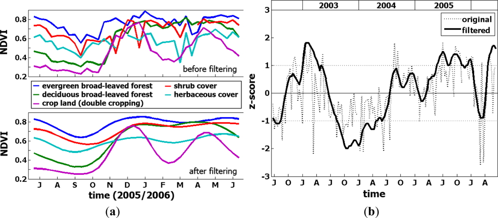
Figure 1. Illustration of positive filtering effects on satellite-derived (10-daily) NDVI time series (from Atzberger and Eilers [31]; modified). For filtering and gap filling, the Whittaker smoother was used. The NDVI time series are from SPOT-VGT. (a) Example NDVI profiles from different land cover types before (top) and after (bottom) smoothing with the Whittaker filter. The profiles were randomly extracted within the state of Mato Grosso in Brazil; (b) Effects of the smoothing on vegetation anomalies (z-scores) over a randomly selected grassland pixel in Mato Grosso (Brazil).
Remotesensing 05 01704f1
Figure 2. Global map of NDVI anomalies during the 2012 growing season (August). Negative anomalies are visible mainly in central US, central Asia and northern Brazil, while a positive situation is evident in eastern China and southern Brazil. Data are from SPOT VEGETATION (as compared to 1999–2010 average). Anomalies are expressed in absolute NDVI units.
Remotesensing 05 01704f2
Figure 3. Z-scores (standardized differences from long term average (LTA)) of cumulated NDVI and rainfall estimates over the two crop seasons (called Gu and Deyr) of an agro-pastoral district in Southern Somalia (Bardera). The two failed seasons in 2010 and 2011, which lead to a major famine in the country are clearly visible. In most cases a major NDVI anomaly is explained by a similar rainfall anomaly, but this is not always the case, as for example in the Gu season of 2003. In such cases temporal distribution of rainfall has to be taken into consideration as well as non-rainfall related factors influencing the NDVI, such as changes in crop area.
Remotesensing 05 01704f3
Figure 4. NDVI/yield linear regressions for cereals in North Africa (from Maselli and Rembold [46]; modified). (Top) Evolution of the coefficient of determination (R2) between radiometric variable and yield over time. (Bottom) Scatter plots between NDVI and cereal yield. Each dot corresponds to the annual yield for agricultural areas at national level and to the monthly NDVI best correlated to yield.
Remotesensing 05 01704f4
Figure 5. Dependence of εb (chickpea) on water stress (Singh and Sri Rama [77], from Atzberger [56]).
Remotesensing 05 01704f5
Figure 6. Linear regression between the seasonally (from sowing to harvest) integrated absorbed PAR and dry matter at harvest (g·m−2) of nine commercial winter wheat plots from Atzberger [56].
Remotesensing 05 01704f6
Figure 7. Simplified scheme of a crop process model. Model state variables such as development phase, organ dry mass, or leaf area index are linked to input variables, including weather, and geographic and management variables (from Delecolle et al.[50]).
Remotesensing 05 01704f7
Figure 8. Schematic description of the re-calibration method using radiometric information as inputs. The crop growth model simulates the leaf development (LAI) over time. This information is used to simulate the canopy reflectance using an appropriate canopy reflectance model. In the non-linear minimization procedure, new model coefficients are assigned to the crop growth model such that the residues between observed and simulated reflectances are minimized (Atzberger [56] from Delecolle et al.[50]).
Remotesensing 05 01704f8
Figure 9. Schematic description of the “forcing” method. The complete time profile of a crop state variable (here: LAI) is reconstructed from remote sensing data and introduced into the dynamic crop growth model at each time step in the simulation (from Delecolle et al.[50]).
Remotesensing 05 01704f9
Table 1. Properties of the most common optical low and medium resolution operational and planned sensors relevant for vegetation monitoring. (The following abbreviations are used for different intervals of the electromagnetic spectrum: VIS = visible, NIR = near infrared, SWIR = short wave infrared, MIR = medium infrared). NB: The ENVISAT mission stopped officially in May 2012.
SensorPlatformSpectral RangeNumber of BandsResolutionSwath WidthRepeat CoverageLaunch
AVHHRNOAA
POES 6–19
VIS, NIR, MIR51,100 m2,400 km12 h1978
AVHRRMETOPVIS, NIR, SWIR, MIR51,100 m2,400 km12 h2007
SEAWIFSOrbview-2VIS, NIR81,100 m
4,500 m
1,500 km
2,800 km
1 day1997
VEGETATIONSPOT 4, 5VIS, NIR, SWIR41,100 m2,200 km1 day1998
MODISEOS
AM1/PM1
VIS, NIR, SWIR, TIR36250–1,000 m2,330 km<2 days1999
MERISENVISATVIS, NIR15300 m (1,200 m)1,150 km<3 days2000
PROBA-VPROBA-VVIS, NIR, SWIR4300 m (1,000 m)2,250 km1 dayForeseen 2014
SENTINEL 3SENTINELVIS, NIR, SWIR21300 m1,270 km<2 daysForeseen 2014
Table 2. Statistical summary of millet grain yield-integrated NDVI regression models for Senegal showing how the model can be improved by introducing additional bio-climatic variables like percentage of cultivated land (AGRIPRC) and Tropical Livestock Unit Density [63]. iNDVI is NDVI integrated from August to October, while iNDVI PAR is monthly values of NDVI and PAR (photosynthetically active solar radiation) multiplied and accumulated for the period July to October.
No.Model ParametersYearr2Standard Error of Estimate kg·ha−aResidual Mean SquareF-ratioTabled F at P < 0.05n
1aiNDVIb19900.60625464,74515.384.9612
2aiNDVI + b19910.73818634,63939.434.6016
3aiNDVI + b90 + 910.64522048,34947.204.2328
4a ∑8iNDVI PAR) + b19900.52328078,35810.974.9612
5a ∑2iNDVI PAR) + b19910.69020240,99531.154.6016
6a ∑6iNDVI PAR) + b90 + 910.202329108,5706.604.2328
7aiNDVI + b
AGRIPRC + c
90 + 910.66020843,24622.303.4226
8aiNDVI + b >
TLUDEN + c
90 + 910.69519738,81526.163.4226
9AGRIPRC >
22.5 aiNDVI+b
90 + 910.72916627,53435.044.6726
10AGRIPRC>
22.5 aiNDVI + b
AGRIPRC + c
90 + 910.81414320,53026.223.8915
11AGRIPRC >
22.5 aiNDVI + b
TLUDEN + c
90 + 910.88311312,85845.443.8915
12AGRIPRC < 22.5
aiNDVI + b
90 + 910.66324459,63721.684.8413
13AGRIPRC <
22.5 aiNDVI + b
AGRIPRC + c
90 + 910.76321244,84612.874.4611
14AGRIPRC <
22.5 aiNDVI + b
TLUDEN + c
90 + 910.68524459,5378.704.4611
AGRIPRC is percentage of cultivated land and TLUDEN is Tropical Livestock Unit Density. The a, b and c are regression coefficients