Improved Sampling for Terrestrial and Mobile Laser Scanner Point Cloud Data

Department of Remote Sensing and Photogrammetry, Finnish Geodetic Institute, Geodeetinrinne 2,FI-02431 Masala, Finland
*
Author to whom correspondence should be addressed.
Remote Sens. 2013, 5(4), 1754-1773; https://doi.org/10.3390/rs5041754
Submission received: 23 January 2013
/
Revised: 4 March 2013
/
Accepted: 27 March 2013
/
Published: 9 April 2013
(This article belongs to the Special Issue Advances in Mobile Laser Scanning and Mobile Mapping)
Abstract
:We introduce and test the performance of two sampling methods that utilize distance distributions of laser point clouds in terrestrial and mobile laser scanning geometries. The methods are leveled histogram sampling and inversely weighted distance sampling. The methods aim to reduce a significant portion of the laser point cloud data while retaining most characteristics of the full point cloud. We test the methods in three case studies in which data were collected using a different terrestrial or mobile laser scanning system in each. Two reference methods, uniform sampling and linear point picking, were used for result comparison. The results demonstrate that correctly selected distance-sensitive sampling techniques allow higher point removal than the references in all the tested case studies.
1. Introduction
Terrestrial laser scanners were first introduced about 15 years ago. Since then, they have been exploited in increasing numbers for a wide variety of research and mapping solutions, both in terrestrial (TLS) and mobile (MLS) laser scanning configurations. They are regularly applied in archaeology [1], geology [2], building modelling and reconstruction [3,4], outdoor object determination [5], and outdoor mapping [6]. TLS has also made a breakthrough in a wide variety of forestry applications, including both forest inventory and ecology applications (e.g., Dassot et al.[7] and references therein). More recently, MLS data combined with RGB information have also been utilized in individual tree species classification on ground level [8].
At present, the properties of both laser ranging units and their supporting instrumentation have grown significantly from their earlier versions. Table 1 illustrates the development of different contemporary laser scanning systems and also gives an overview of their general properties. More extensive scanner comparisons and descriptions can be found in detailed product surveys (e.g., by Lemmens [9,10]) and in laser scanning text books (e.g., Shan & Toth or Vosselman & Maas [11,12]). The table shows how laser scanner measurement frequencies and maximum ranges have increased steadily. Improved measurement capability also means that the dataset sizes have grown correspondingly as a result of higher number of points, better accuracy, and additional point information such as individual point intensities or their return numbers. Nevertheless, the raw computing power and data storage sizes have also increased along with the growing dataset sizes, thus compensating for the burden.
However, in cases where a scanner is on ground level and it scans over a wide solid angle around it, it is possible that the number of laser points may become locally higher than needed for analysis. Furthermore, the scanning geometry causes a large variance within the point cloud and makes algorithm parametrization difficult. For example, such scanning scenes are often located in forest environments where a scanner is surrounded with vegetation and other natural targets with irregular shapes. Local point densities can also be considered higher than required in the built environment if measurements are carried out to capture the general properties of the area, e.g., to determine object locations and their rough outlines, and when accurate object modelling is not the main priority. As point cloud processing performance is directly dependant on the available number of points, this means that a higher than required number of points is disadvantageous for data processing and therefore slows it down. The same holds for data storage: once the local point density reaches its application-specific limit, additional points will still require storage space without adding significant information to the analysis.
High number of points is mainly a problem with close-to-medium range TLS and MLS systems with wide scanning angles. Figure 1 illustrates typical scanning geometries of a stationary terrestrial and a mobile laser scanning system. The terrestrial scanning geometry illustrated in Figure 1(a) is a spherical one and it is collected with scanners that have two freely rotating axes. The mobile case in Figure 1(b) demonstrates the scanning geometry of a fully rotating single laser scanner mounted on a moving vehicle. The scanning plane is typically circular or elliptical depending on the tilt of the scanner with respect to the axis of the trajectory. When the platform moves, the formed point cloud can be described as a helix or a cylinder depending on the platform direction and velocity. In both geometries, the structural properties of the scanner or the platform often limit available scanning angles to some extent.
Local point densities in the vicinity of both scanner types might rise over hundreds of thousands of points per square meter (e.g., see Litkey et al.[25]). This is because they both usually collect data with evenly spaced angular steps, resulting in a uniformly distributed point cloud representation with respect to scanning angles. However, since the scanners are located within the study scene in both geometries, the ground and nearby objects cover a significant portion of the solid angle around the scanner. This leads to a significant variance in point density on target surfaces. The extent of the variance depends on the surface distance from the scanner.
In cases where all the measured data needs to be saved, one of the best approaches is to use memory efficient data formats. These take into account the special characteristics of the data and can thus save each point in a small space. Both commercial and openly accessible formats have been developed for this purpose. One of the most popular open formats for saving laser point data is the binary LAS [26]. Furthermore, laser point clouds saved in LAS format can be packed further with proper encoding as Isenburg, and Mongus and Žalik have demonstrated [27,28]. The LAS format is mainly developed and used for saving airborne data, but it can be also utilized for the storage of TLS data. Recently, another data format, ASTM E57, has been introduced [29]. The main aim of ASTM E57 is to store 3D imaging system data on a more general level. For this purpose, the format is designed to provide a flexible means for storing both laser point cloud and imagery data regardless of the scanner system.
Another space-saving approach is to compress 3D point cloud information using octrees [30–32]. Octrees divide the point cloud area into equally sized cubes, which are further divided into eight child cubes. The branching is continued until the maximum branching level, controlled by cube size and number of points within a cube, is reached. Octrees have been used in computer graphics for a long time to present volumetric data (cf. [30,33] and their references). The branching structure and inherent neighbourhood information of octrees also allow fast access to data on point level.
If point removal is allowed, dataset sizes can be reduced in several ways, either during measurements or during data processing. During measurements, it is possible to limit scanning angles so that hits from the immediate vicinity of the scanner are excluded. However, hard thresholds remove all points from the excluded area, which may leave out important data. Hard thresholding also causes discontinuities, which may cause additional problems if data are used for interpolation, fitting, or when the dataset is georeferenced with other datasets.
Another method for reducing data during measurements is to set a suitable scanning resolution. When the targets of interest are scanned from a distance, the possible overlap between neighbouring laser points increases. This happens because the laser footprint increases as a function of distance due to laser beam divergence, but the sampling interval remains constant. This effect becomes important and should be tested for if the scanning is performed from a distance, and especially with limited fields of view. Detailed discussion of laser footprint sizes and test cases can be found in articles by Lichti and Jamtsho and by Pesci et al.[34,35]. In this paper, possible point overlap effects were not accounted for in data analysis as all range distances were relatively short, i.e., within 30 m, to the scanners.
During processing, dataset size reduction can be achieved by sampling the point cloud with a suitable filtering algorithm. A straightforward way to perform this is to take a uniform sample of the data. However, point densities in the previously mentioned TLS and MLS scanning geometries have strong distance dependency and they drop rapidly when the distance to the scanner increases. In other terms, if one creates a distance distribution of all point distances to the scanner, it will have a dominant peak at close range. When the point cloud is sampled uniformly, then the distance distribution of the sampled point cloud resembles the shape of the full data distribution. Figure 2(a) illustrates this with a synthetic example. As the distance distribution shape is retained, it means that point densities drop by the same amount in all distances. Therefore, the high density parts of the point cloud will still have the most points. However, lower point densities, in general, mean that the effective range for detecting objects of interest decreases. This decreases the usability of uniform sampling as the loss of effective scanning range requires that additional measurements and data registrations have to be carried out.
In addition to the straightforward hard thresholding and uniform point sampling, various other computational techniques have been developed to reduce point cloud sizes. These include: utilization of local geometry representations to search for and remove redundant points from object surfaces [36]; projections of rigid and adaptive grids on object surfaces [37]; point cloud measure-direction equalization with the use of sensor characteristics [38]; and range-dependent median filtering along 2D scan lines [39]. The first two techniques utilize point-to-point or neighbouring point distances in analysis, which allows high quality object sampling but is computationally heavy. The third technique samples the whole point cloud. The fourth technique uses the median values of consecutively measured points along each scan line, making it very fast.
In this paper, the main aims are to present two sampling methods and to test their efficiency for improving data utilization. The sampling methods use point cloud distance distributions of the whole point cloud to reduce data size. The methods are quick to perform and they require only a little prior knowledge of the scanned area and the scanning configuration. Method efficiency is evaluated in three separate case studies in which data were collected with a different laser scanning system in each case. The paper focuses on the sampling methods and how they affect data processing. Therefore, the case studies were selected from earlier experiments to utilize known processing algorithms and their results. This approach also allows us to inspect how the processing algorithms are affected by different sampling methods. In addition, the paper also aims to: (i) discuss the differences detected between the results in the case studies; and (ii) suggest possible improvements for future research.
The rest of the paper is structured as follows: first, the sampling methods and their references are described; second, results from three separate case studies are presented and reviewed; and third, the studies and their results are summarized.
2. Sampling Method Descriptions
This section presents the algorithms of the two reference and the two range-based sampling methods. To guarantee result comparability between the methods in each case study, the following laser point selection rules were applied in all cases. The first rule was that a single laser point could be picked only once in each subsample. The second rule was that the size of each subsample, within rounding limits, had to be preserved. This meant that if the wanted number of laser points were not available in a selected part of a distance distribution, the remaining points were picked from other parts of the distribution.
2.1. Reference Methods: Uniform Point Sampling and Linear Point Selection
The uniform point sampling was performed by taking a randomly selected sample of the wanted size (Sn) from the full data of size Stot so that Sn = n × Stot, where n is the wanted sampling ratio (0 < n < 1). It is referred to with a label “nr” in text. The uniformly sampled data distributions of a synthetic test point cloud are shown on the left side of Figure 2(a). The figure shows that the shapes of the uniformly sampled point distance distributions retain the shape of the original distance distribution. If the sampling was performed by taking every
:th point from the full data instead, the resulting shapes of the sampled distributions would have been almost the same, e.g., for n = 0 25 the Sn would be 1, 5, 9, …, N. This linear point selection, referred to as ‘nl’ in the text, was chosen as the second reference method.
2.2. Leveled Histogram Sampling
The leveled histogram sampling, referred as “lh” in the text, aims to collect scanned points evenly from all distances. Resulting histogram shapes with 20% and 50% sampling ratios are illustrated in the center of Figure 2. As Figure 2(b) shows, the resulting sampling distribution is artificially flat. This sampling method is based on the assumption that all parts of a point cloud distribution are likely to carry information in them even if their total number of points is low. On the other hand, distribution parts with a very high point count are likely to have excessive points that do not add to the information content. Therefore, part of them can be removed with no significant effect on the analysis result. The point selection in high density parts of the distribution is performed uniformly as individual points are not assumed to have critical information in them.
The algorithm requires two control parameters, the sample size and histogram bin width. The sampling algorithm is as follows:
- Calculate a histogram with even-width bins from point cloud data with Nb bins and calculate the number of the sample points Snb in each bin so that .
- Select all points located in bins with less than Snb points in them and deduct their number from the Sn. Calculate the number of possible excess points, Nex, so that , where Sbin;i is the number of points in a bin with less than Snb points and the l is the index of all such bins.
- Divide the excess number of points evenly into the remaining bins so that Snb(2) = Snb(1) + Nex(1), where the number in parenthesis is the iteration step count.
- Repeat steps 2 and 3 until all remaining bins have more than Snb(m) points, where m is the total number of iterations.
- Select Snb(m) random points from each remaining bin so that the sum of all selected points totals Sn.
2.3. Inversely Weighted Distance Sampling, Two and Three Dimensional Cases
Inversely weighted distance sampling draws its idea from spherical volume point picking (e.g., in [40]), but uses it in an inverted way. Instead of generating uniformly distributed random points within a space, random numbers are generated and range-weighted inversely to pick individual points randomly from the point cloud. Inverse weights are set for points based on the assumed point cloud distribution. Here, uniform point cloud distributions within a disk and within a sphere were assumed corresponding to a two- and three-dimensional case, respectively. The cases are labeled as “s2d” and “s3d” in the text. The point weighting was carried out by determining a point rank number as: Pr = ⌊Stot × U1/d⌋ + 1, where Stot is the total number of points, U is a uniformly distributed random number (0 < U ≤ 1), d is the selected dimension, and the brackets mark the floor function. The selection algorithm is as follows:
- Sort every point in the point cloud according to their distance (2D or 3D) from the scanner.
- Generate a uniformly distributed random number (U) and weight it inversely to calculate a weighted random point rank number (Pr).
- Select the point with the corresponding rank number, move it to a selected point list, and update the remaining point list.
- Repeat steps 2 and 3 until Sn points are picked.
Figure 2(c) shows how the resulting distribution of the sampled (a 3D case) point cloud is heavily weighted on the distant side of the distribution, while the number of points close to the scanner is reduced significantly.
3. Evaluation of Sampling Methods in Three Case Studies
To evaluate the performances of the different sampling methods, they were tested in three separate case studies. The case studies were reference target detection from a TLS dataset, pole-like object detection from an MLS dataset, and wall detection from another MLS dataset. The case studies were selected to represent a variety of different laser scanning applications and configurations as this allowed to study how the sampling methods, different scanning geometries, environments, and data collection techniques affect together the full data processing chain.
In each case study, a dataset was first collected with a different TLS or MLS platform. After possible pre-processing steps, new datasets were created by sampling the full dataset with each sampling method and with several sampling ratios each. Then, the new datasets were processed with a case study specific algorithm. The algorithm parametrization was kept constant in each run. This approach was chosen to limit changes in results and processing times only on the effects depending on sampling ratios and point cloud selection methods. Finally, the results and processing times obtained with different sampling methods and ratios were compared against those obtained with the full point cloud. All sampling and analysis were carried out with MATLAB (MathWorks Inc., Natick, MA, USA).
The method performance was evaluated with two main criteria. The first evaluation criterion was the preservation of the full-data result obtained with a case study specific algorithm. Ideally, a good sampling method would result in data subsamples whose properties remain close to those of the full data as long as possible when the sampling ratio is lowered. This would imply that the sampling method is successfully reducing points from high density areas while preserving the information content of the others. The second criterion was the change in the total processing time, including the time spent in sampling. The results for both criteria are reported with respect to the full data results in each case study.
3.1. Case Study I: Spherical Reference Target Detection in a Forest Environment from TLS Data
3.1.1. Study Object and Reference Target Detection Description
The objective of Case Study I was to determine the maximum range in which a spherical reference target could be detected and how sampling with different methods affects the maximum detection range. The study was carried out by planting 10 high reflectance reference spheres in a forest plot area. The diameter of a single reference sphere was 145 mm. Reference targets are used in terrestrial scanning to register different scans (i.e., to align them) with the reference coordinate frame and with each other.
Reference target detection was determined by counting the number of hits on them. Outlines of the targets were manually set using full point cloud. At least 30 hits were required to guarantee a reliable detection of a reference sphere with low spatial uncertainty. The farthest sphere-scanner distance was 25.8 m, which was within the theoretical detection range of 43.7 m. To guarantee possible detection of all reference spheres, a 27.0 m horizontal threshold range was set around each scanner. As all spheres were within the theoretical detection distance, the maximum number of visible reference spheres was 70 if each sphere would have been visible to every scanning location. However, all spheres were not visible to every scanner location due to occlusions within the plot.
3.1.2. Data and Measurement Descriptions
Data for Case Study I consisted of seven TLS point clouds. Scans were taken from a single forest plot in May 2010 in Evo, Finland. One scan was performed in the middle of the plot and the other six scans were measured from the edges of the plot, between 10 and 14 m from the plot center, with 60 degree spacing. A Leica HDS6100 (Leica Geosystems AG, Switzerland) terrestrial laser scanner was used for the measurements. The scanner transmits a continuous laser beam (wavelength 650–690 nm) and determines distance based on the detected phase difference. The maximum measurement range of the scanner was 79 m. The distance measurement accuracy is 2–3 mm up to 25 m. The field-of-view (FOV) of the scanner is 360° × 310°. The transmitted beam is circular and it has a 3 mm diameter at the exit. The beam divergence is 0.22 mrad. The used measurement resolution produces 43.6 M (million) laser points in the FOV, and the point spacing is 6.3 mm at a distance of 10 m. Each scan consisted of approximately 31.5 M points after pre-filtering. All scans were pre-filtered with a default filter included in the scanner import software, Leica Cyclone, before sampling. The filter removes points with low intensity, downward angle, and range, as well as points that are near an object egde (mixed) or isolated.
3.1.3. Sampling Results
The results of Case Study I are illustrated in Figure 3. A total of 57 reference spheres were visible to all scanners out of a possible 70 in the full data. The farthest detected sphere was located 23.6 m away from a scanner. Figure 3(a,b) illustrates a point cloud of a single scan and its distance distribution. Point clouds of other scans had similar distribution shapes. As Figure 3(b) shows, the distance distribution is mainly concentrated near the scanner. The shape of the distribution implies that sampling techniques sensitive to point distances should obtain similar results to those with the full data when using a low number of sampled points.
Figure 3(c,d) shows that all reference spheres were already detected with a sampling ratio of 20% with the “lh” method and that all different sampling methods detected over 90% of the possible targets with the 50% sampling ratio. The best performing sampling method, “lh”, detected 50 out of 57 targets already at a sampling ratio of 10%. With uniform (nr) and linear (nl) sampling, a 40% sampling ratio was required to reach the same detection level. The performance of distance-weighting sampling methods (s2d and s3d) was between those of the uniform and the leveled histogram methods.
Additionally, the distance of the farthest detected target was tested using each sampling method and ratio (Figure 3(d)). Here, the leveled histogram (lh) method is clearly the best-performing. It can detect the farthest target already at a 10% sampling ratio and a target over 20 m away already at the 5% sampling ratio. The second-best performing sampling method is the distance-weighting method (s3d) that obtains respective results at sampling ratios of 30% and 10%. The reference methods obtained over a 20-meter detection distance at a sampling ratio of 40%.
The time required for point sampling varied from under one second with the linear point selection (nl) to close to 30 seconds with the 3D distance-weighting method (s3d). When compared against the processing times of other processing steps, such as data loading times and point delineation from the point cloud, the sampling times were below 10% of the whole processing time in all cases.
3.2. Case Study II: Pole and Tree Trunk Detection in an Urban Environment from MLS Data (FGI Roamer)
3.2.1. Study Object and the Algorithm Description
The objective of the second case study was to compare the number of pole shaped objects detected from an urban street environment. False detections were not of interest in this study as it was assumed that point cloud subsampling would not have increased the false positive ratio.
The pole detection algorithm applied in Case Study II detects first individual segments from data to find candidate clusters whose shape resembles poles and trunks [41]. The candidates were then classified either into “pole-like” or “other” object classes based on five attributes. The algorithm requires that the scanning plane is tilted with respect to both vertical and driving directions. With this configuration, several short sweeps were measured from each vertical pole-like object that was longer than a preset length threshold. First, the algorithm segments the data along scan lines (each scan line individually) to find short point groups that resembled sweeps reflecting from poles. Then, point groups were clustered and groups on top of each other were searched for from adjacent scan lines. Before classification, the clusters were merged if needed. Clusters were then classified as “pole-like” and “others” classes using a five-step decision tree. Classification attributes included the cluster shape, cluster orientation, cluster length, number of sweeps in the cluster, and local point distribution around the cluster [41].
3.2.2. The Data Description and Reference Results
The data were collected with an FGI Roamer mobile mapping system. It contains a Faro Photon™ 80 phase-based laser scanner and a NovAtel SPAN™ navigation system that are fitted to a rigid platform, which can be mounted on a car. Faro scans 2D profiles with a field of view of 320° in a scanning plane and the motion of the vehicle provides the third dimension. Comprehensive measurement system specifications are described in detail in earlier studies by Kukko et al. and Lehtomäki et al.[42,43]. The test area was a location in the city of Espoo, southern Finland, and it is one of the EuroSDR test fields [44].
The dataset was collected with a 48 Hz scanning frequency and it consisted of 8.2 M laser points. The reference contained 538 tree trunks, traffic signs, traffic lights, lamp posts, parking meters, and other poles. Object locations were picked manually from dense terrestrial reference scans. The reference was limited to closer than 30 m from the trajectory and to objects taller than one meter. Earlier studies in the EuroSDR test field had shown that the detection rate of the algorithm was 51.8% for all targets [43].
3.2.3. Sampling Results
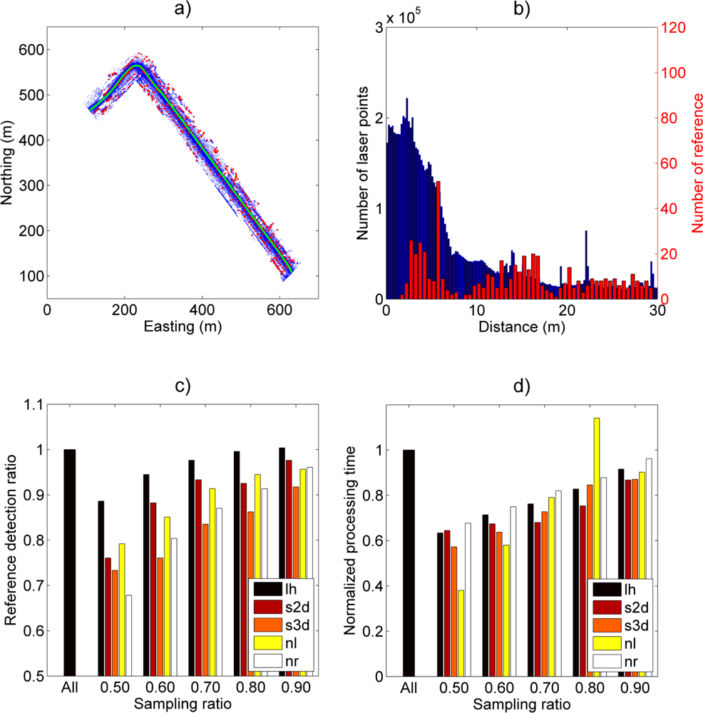
The results of Case Study II are illustrated in Figure 4. Figure 4(a) illustrates the point cloud with pole-like objects marked with red, and the scanner trajectory marked with green. The point cloud distance and the target distance distributions are shown in Figure 4(b). The target distance distribution shows how around one third of the poles are located within a 10 m horizontal distance from the scanner trajectory. The point cloud distribution is again concentrated close to the scanner, but not as pronouncedly as in Case Study I in which a stationary scanner was used.
Figure 4(c) shows the effect of a sampling ratio in the pole detection against the case with the full data. Changes in pole detection performance resemble each other more than in Case Study I as the pole detection rate remains higher than the sampling ratio for all sampling methods. Overall, the leveled histogram (lh) performs the best among all methods when the sampling ratio was 50% or above. The best individual performance/sampling ratio for the leveled histogram (lh) method is around 60% sampling ratio where it still achieves 94.5% performance compared with the full data result. Below a 50% sampling ratio, the performance of all sampling methods deteriorates so low that utilizing their results would not be feasible in practical analysis.
The total processing time results, normalized against the full data result, are shown in Figure 4(d). The processing times drop in a relatively linear fashion for all methods. However, the linear point selection method (nl) showed a clear deviation from this trend at an 80% sampling ratio. This effect was most likely caused by the pole detection algorithm after it encountered complicated point configurations in the sampled point data. This conclusion was based on a comparison made between the sampling and the pole-searching times.
When inspecting the results, it must be kept in mind that they have been normalized against the results obtained with the full data. This means that the absolute values of pole detection ratios are lower than presented in Figure 4(c). Therefore, determining a suitable sampling ratio for a practical application has to be resolved case-by-case.
3.3. Case Study III: Wall Detection in an Urban Environment from MLS Data (FGI Sensei)
3.3.1. Study Object and the Algorithm Description
The third case study tested the effects of different sampling techniques on a wall detection algorithm developed for mobile laser scanner data by Zhu et al. [4]. The algorithm filters first for noise points using returning pulse widths and isolated points with height statistics. Then, it searches for ground points within the data. The ground points are classified with a grid search that uses height minima of local bins and point cloud height statistics. After ground level determination, walls and buildings are extracted from the data using a two-pass wall detection algorithm: The algorithm creates a binary image of the area using the overlap between two grid layers taken from different heights and then searches for lines within the image. Tall buildings are detected during the first pass and low buildings during the second pass. Laser points located within the line pixels of the binary image are labeled as wall points.
3.3.2. The Data Description and Reference Results
The dataset was collected with a low-cost mobile mapping system, Sensei. The Sensei system is built at the Finnish Geodetic Institute and it has been utilised in road-side mapping studies [8,45]. The measurement configuration consisted of an Ibeo Lux laser scanner (Ibeo Automotive Systems GmbH, Hamburg, Germany), a Novatel 702 GG GPS receiver (NovAtel Inc., Calgary, AB, Canada), and a Novatel SPAN-CPT inertial navigation system. The Sensei system can also carry an imaging system, but this was not utilised in the current case study. The laser scanner is capable of collecting 38,000 pts/s over a 110° opening angle.
The dataset was collected from a residential area located in Kirkkonummi, southern Finland. The area consists of one- and two-story houses. The dataset covered about 6,900 m of roadside environment with partial overlap. The dataset contained about 9.0 M points after noise point filtration. Out of these points, 4.4 M were classified as ground points and 1.9 M points were classified as wall points. The rest of the above-ground points were not used in analysis.
3.3.3. Sampling Results
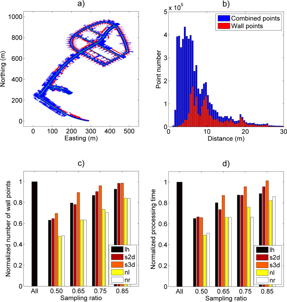
An illustration of Case Study III and its results are presented in Figure 5. Figure 5(a,b) shows the study area and the point distance distribution of the wall points and the combined wall and ground points. The blue color represents the combined points and the red color represents the wall points as detected by the algorithm. The laser scanner trajectory is colored with green in Figure 5(a). Inspection of the distance distributions shows that the analyzed point cloud consists mainly of wall points as the distance to the scanner increases. This was expected as the scanner trajectory was located in a densely built area with low vegetation. However, points close to the scanner were mainly ground hits.
The normalized wall point ratio in Figure 5(c) shows that sampling methods utilising inverse distance weighting have the best performance for this kind of distance distribution. The inverse three-dimensional distance weighting (s3d) performed the best among all methods by including 90% of the wall points detected from the full dataset with a 65% sampling ratio. This was expected as the method puts most weight on the most distant points. A corresponding two-dimensional method (s2d) and leveled histogram sampling (lh) had similar performance when compared against each other, but their performance was clearly below that of the inverse 3D distance weighting (s3d). Uniform (nr) and linear (nl) point selection methods resulted in a close to linear response in wall point detection and their performances were clearly lower than with other techniques.
The processing times measured during wall determination were longer with the new sampling methods than with the reference methods. The main reason for this was most likely within the wall point search routine. This estimation is based on comparing the ratio of found wall points against the total processing time (Figure 5(c,d)). The figures show that there was a close resemblance between the wall point ratio and total processing time. This would imply that the total processing time depends heavily on the final number of found wall points regardless of the sampling ratio (e.g., compare method “s3d” wall point ratios and processing times at sampling ratios from 65% to 85%).
4. Discussion
The results of Case Studies I–III demonstrate that the implementation of straightforward sampling methods retains most of the required information content of data while saving both processing time and data storage space. This is important as it means that a point cloud can be sampled efficiently by knowing only its general distance characteristics. Furthermore, unsupervised sampling methods can be integrated tightly into data processing chains. This should give significant benefits when data are collected operatively on a large scale. The results also imply that the best sampling method and ratio are dependent on the application requirements, so case-by-case testing for the best sampling method is recommended.
Moreover, it is possible to lower the effective sampling ratios as low as 10% of the full data size in a good case as Case Study I demonstrates. However, in Case Studies II and III, where scanners were mounted on mobile mapping systems and the objects of interest consisted of more points and more complex shapes, the most effective sampling ratios—in terms of overall point count and processing time speed-up—were found already at around 60% of the full data. Below that ratio, the sampled point clouds lost so much information content that it was no longer feasible to use those clouds for target detection. This highlights the need to consider carefully which type of sampling method would save the information content best, and what would be the minimal level of the needed information content, i.e., the sampling ratio, before processing large areas.
It was also shown that the efficiency of a particular sampling method depends on the shape of the point cloud distance distribution of the targets of interest. For example, in Case Studies I and II, the targets of interest were located evenly along the distance axis. In these cases, the leveled histogram (lh) approach had the best performance. On the other hand, when the object points were located away from the scanner, as in Case Study III, the inverse distance weighting methods retained most of the object information. In general, both proposed sampling methods retained information better than the two reference methods, namely uniform point sampling (nr) and linear point selection (nl).
While the new sampling methods are able to save the information content of data better than uniform and linear sampling, the gains in total processing times were not that clear. The sampling processes took only a small percentage of the total processing time in each case study, which implied that the processing algorithms themselves were sensitive to the spatial distribution of point clouds. A possible explanation for this is that the new sampling methods were designed to preserve distant points. Thus, the processing algorithms had to analyse larger areas, which in turn slowed them down. This conclusion was further backed up by the fact that the processing times in both uniformly and linearly sampled point clouds, which reduce effective scanning range, scaled nearly linearly with the number of points in all case studies.
It was also observed that processing algorithms might have occasional sensitivity to individual sampling method and point ratio combinations, i.e., in Case Study II. In such a case, the total processing times might be significantly longer than would be otherwise expected.
Overall, when changes in both analysis performance and in total processing times are taken into account in all case studies, the results show that distance distribution-based sampling methods retain information content better than uniform or linear sampling. However, the sampling method, analysis algorithm, and its parametrization all have a cumulative effect on the final result. Therefore, prior testing is still required before processing large datasets. Nevertheless, it is possible to reduce point cloud sizes quite safely by tens of percents with a properly selected and parametrized sampling method, and still retain most of the target information. We also assume that more specialized distribution-based sampling approaches could allow even higher point reductions.
To sum up the results, the leveled histogram (lh) sampling gave the best general performance in the case studies. If most of the objects are known to be distributed away from a scanner, then sampling with inversely weighted distance sampling is likely to yield the best results. The strength of the range-based sampling methods is that they can be applied quickly and in principle to most types of TLS and MLS data. However, since the methods are based on point cloud statistics i.e., they treat the point cloud as a whole, there are limitations that need to be considered. First, the methods do not account for the neighbourhood information of individual points. While this saves processing time, it reduces the method suitability for studies where high point densities are required to preserve detail, e.g., in accurate building facade extraction and modeling [46–48], or in road marker detection and mapping [49,50]. Reviews by Rottensteiner (2012) and by Wang and Jie (2009) give comprehensive overviews about the common techniques used in solving these problems [51,52]. Second, the point cloud should be such that it can be described with a relatively smooth distance distribution, i.e., the point cloud spatial dimensions should be large compared with object sizes. These limitations mean that the presented methods are the best suited for scanning configurations where short-to-medium scanning ranges and a wide solid angle are used, and where the main goal is in locating and extracting the general shape of objects of interest.
5. Conclusions
In this paper, we propose two sampling approaches to reduce point cloud data while retaining most of the information content of the full dataset. The data reduction is achieved with efficient point cloud sampling methods that use the information about the data collection geometry i.e., point cloud distance distributions. The sampling methods were tested in three separate case studies in which data were collected with a different sensor system in each case. Multiple case studies allowed the study of the combined effects of the sapling methods, different scanning geometries, environments, and data collection techniques on study outcomes.
In conclusion, the results obtained with the new sampling methods were promising. The leveled histogram (lh) and inverted distance weighting (s2d, s3d) performed better than their references in all three case studies. Moreover, none of the new sampling method implementations was particularly optimized for any of the case studies. Because of this, we expect that the implementation of more advanced sampling techniques is possible and that they are likely to yield even better data processing performance and allow high-level integration in data processing chains. The new sampling methods demonstrated in this article were carried out using only point cloud distance distributions. It would be of interest to test if there are other point cloud statistics that could be sampled with a similar approach. Additionally, if such statistics are found, it would be of interest to test the effect of combining or using different sampling methods consecutively. This would possibly allow even further dataset size reductions while preserving most of the required information content.
At present, the demand for accurate geoinformation data continues to increase rapidly with growing commercial and social interest. This means that larger areas will be scanned with high resolution on an operative scale, both outdoors and indoors. Additionally, laser scanning techniques continue to improve all the time and the new scanner systems are faster and have a longer range than their predecessors. Furthermore, new types of scanners are also emerging: multiple wavelength and hyperspectral laser scanners that are able to collect both spatial and spectral information simultaneously [53–55]. Moreover, some of these systems collect spectral data with full waveform. All these improvements and new properties mean that dataset sizes are likely to grow significantly when compared with the present situation. As a result, new sampling methods that improve the processing efficiency of continually growing point clouds will be of interest in the coming years as their demand will grow in both TLS and MLS. Therefore, it is imperative that efficient and information-preserving data sampling methods are already being developed to guarantee efficient exploitation of these novel laser scanning systems when they reach operative capability.
Acknowledgments
The authors would like to acknowledge The Academy of Finland for its financial support in the form of the projects “Science and Technology Towards Precision Forestry”, “Towards Improved Characterization of Map Objects”, “Economy and technology of a global peer produced 3D geographical information system in built environment-3DGIS”, “Interaction of Lidar/Radar Beams with Forests Using Mini-UAV and Mobile Forest Tomography”, and “New techniques in active remote sensing: hyperspectral laser in environmental change detection”. The authors thank reviewers for their comments and suggestions.
References
- Vozikis, G.; Haring, A.; Vozikis, E.; Kraus, K. Laser Scanning: A New Method for Recording and Documentation in Archaeology. Proceedings of the Workshop-Archaeological Surveys, WSA1 Recording Methods, FIG Working Week, Athens, Greece, 22–27 May 2004; 4, p. 16.
- Buckley, S.; Howell, J.; Enge, H.; Kurz, T. Terrestrial laser scanning in geology: Data acquisition, processing and accuracy considerations. J. Geol. Soc 2008, 165, 625–638. [Google Scholar]
- Gross, H.; Thoennessen, U. Extraction of Lines from Laser Point Clouds. Proceedings of the Symposium of ISPRS Commission III: Photogrammetric Computer Vision PCV06, Bonn, Germany, 20–22 September 2006; 36, pp. 86–91.
- Zhu, L.; Hyyppä, J.; Kukko, A.; Kaartinen, H.; Chen, R. Photorealistic building reconstruction from mobile laser scanning data. Remote Sens 2011, 3, 1406–1426. [Google Scholar]
- Lim, E.; Suter, D. 3D terrestrial LIDAR classifications with super-voxels and multi-scale Conditional Random Fields. Comput. Aid. Des 2009, 41, 701–710. [Google Scholar]
- Petrie, G. Mobile mapping systems: An introduction to the technology. GeoInformatics 2010, 13, 32–43. [Google Scholar]
- Dassot, M.; Constant, T.; Fournier, M. The use of terrestrial LiDAR technology in forest science: Application fields, benefits and challenges. Ann. For. Sci 2011, 68, 959–974. [Google Scholar]
- Puttonen, E.; Jaakkola, A.; Litkey, P.; Hyyppä, J. Tree classification with fused mobile laser scanning and hyperspectral data. Sensors 2011, 11, 5158–5182. [Google Scholar]
- Lemmens, M. Terrestrial laser scanners. GIM Int 2007, 21, 41–45. [Google Scholar]
- Lemmens, M. Terrestrial laser scanners. GIM Int 2009, 23, 62–67. [Google Scholar]
- Shan, J.; Toth, C.E. Topographic Laser Ranging and Scanning: Principles and Processing; CRC Press: Boca Raton, FL, USA, 2009. [Google Scholar]
- Vosselman, G.; Maas, H.-G. Airborne and Terrestrial Laser Scanning; Whittles: Dunbeath, UK, 2010. [Google Scholar]
- Foltz, L. Application: 3D laser scanner provides benefits for PennDOT bridge and rockface surveys. Prof. Surv 2000, 20, 22–28. [Google Scholar]
- Manandhar, D.; Shibasaki, R. Vehicle-Borne Laser Mapping System (VLMS) for 3-D Urban GIS Database. Proceedings of the Computers in Urban Planning and Management (CUPUM) 2001, Honolulu, HI, USA, 18–21 July 2001; p. 10.
- Stephan, A.; Heinz, I.; Mettenleiter, M.; Hartl, F.; Frohlich, C. Interactive Modelling of 3D-Environments. Proceedings of the 11th IEEE International Workshop on Robot and Human Interactive Communication, Berlin, Germany, 25–27 September 2002; pp. 530–535.
- Strecha, C.; von Hansen, W.; van Gool, L.; Thoennessen, U. Multi-view Stereo and LiDAR for Outdoor Scene Modelling. Proceedings of the International Archives of Photogrammetry, Remote Sensing and Spatial Information Sciences, Munich, Germany, 19–21 September 2007; 36, pp. 167–172.
- Gaisecker, T. Pinchango Alto-3D Archaeology Documentation Using the Hybrid 3D Laser Scan System of RIEGL. In Recording, Modeling and Visualization of Cultural Heritage; Baltsavias, E., Gruen, A., van Gool, L., Pateraki, M., Eds.; Taylor & Francis: London, UK, 2006; pp. 459–464. [Google Scholar]
- Boccardo, P.; Comoglio, G. New methodologies for architectural photogrammetric survey. Int. Arch. Photogramm. Remote Sens 2000, 33, 70–75. [Google Scholar]
- Talaya, J.; Alamus, R.; Bosch, E.; Serra, A.; Kornus, W.; Baron, A. Integration of a Terrestrial Laser Scanner with GPS/IMU Orientation Sensors. Proceedings of the XXth ISPRS Congress, Istanbul, Turkey, 12–23 July 2004; 35, pp. 1049–1055.
- FARO Inc. Designed for High Performance: The FARO Laser Scanner LS. Available online: http://www.faro.com/FaroIP/Files/File/Techsheets%20Download/SEA_Laserscanner840&880.pdf (accessed on 13 January 2013).
- Optech Inc. Lynx Mobile Mapper: Summary Specification Sheet. Available online: http://www.optech.ca/pdf/LynxSpecSheet110309Web.pdf (accessed on 13 January 2013).
- Leica GeoSystems AG. Leica ScanStation P20: Product Specifications. Available online: http://www.leica-geosystems.com/downloads123/hds/hds/ScanStationP20/brochures-datasheet/LeicaScanStationP20DATen.pdf (accessed on 13 January 2013).
- FARO Inc. FARO Laser Scanner Focus 3D. Available online: http://www.faro.com/site/resources/share/944 (accessed on 13 January 2013).
- RIEGL Gmbh. VZ-400: Datasheet. Available online: http://www.riegl.com/uploads/tx_pxpriegldownloads/10DataSheet_VZ-400_01-02-2013.pdf (accessed on 26 February 2013).
- Litkey, P.; Puttonen, E.; Liang, X. Comparison of Point Cloud Data Reduction Methods in Single-Scan TLS for Finding Tree Stems in Forest. Proceedings of SilviLaser 2011, 11th International Conference on LiDAR Applications for Assessing Forest Ecosystems, Hobart, Tasmania, Australia, 16–20 October 2011; pp. 626–635.
- ASPRS. LAS Specification, Version 1.4-r11. Available online: http://www.asprs.org/a/society/committees/standards/LAS_1_4_r11.pdf (accessed on 13 January 2013).
- Isenburg, M. LASzip: Lossless Compression of LiDAR Data. Available online: http://www.cs.unc.edu/~isenburg/lastools/download/laszip.pdf (accessed on 13 January 2013).
- Mongus, D.; Žalik, B. Efficient method for lossless LiDAR data compression. Int. J. Remote Sens 2011, 32, 2507–2518. [Google Scholar]
- Huber, D. The ASTM E57 file format for 3D imaging data exchange. Proc. SPIE 2011. [Google Scholar] [CrossRef]
- Elseberg, J.; Borrmann, D.; Nuchter, A. Efficient Processing of Large 3D Point Clouds. Proceedings of the 2011 XXIII International Symposium on Information, Communication and Automation Technologies (ICAT), Sarajevo, Bosnia, 27–29 October 2011; pp. 1–7.
- Schnabel, R.; Klein, R. Octree-Based Point-Cloud Compression. Proceedings of the IEEE/Eurographics Symposium on Point-Based Graphics, Boston, MA, USA, 29–30 July 2006; pp. 111–120.
- Sim, J.Y.; Lee, S.U.; Kim, C.S. Construction of Regular 3D Point Clouds Using Octree Partitioning and Resampling. Proceedings of IEEE International Symposium on the Circuits and Systems, 2005 (ISCAS 2005), Kobe, Japan, 23–26 May 2005; pp. 956–959.
- Laine, S.; Karras, T. Efficient sparse voxel octrees. IEEE Trans. Vis. Comput. Graph 2011, 17, 1048–1059. [Google Scholar]
- Lichti, D.; Jamtsho, S. Angular resolution of terrestrial laser scanners. Photogramm. Rec 2006, 21, 141–160. [Google Scholar]
- Pesci, A.; Teza, G.; Bonali, E. Terrestrial laser scanner resolution: Numerical simulations and experiments on spatial sampling optimization. Remote Sens 2011, 3, 167–184. [Google Scholar]
- Song, H.; Feng, H.Y. A progressive point cloud simplification algorithm with preserved sharp edge data. Int. J. Adv. Manuf. Technol 2009, 45, 583–592. [Google Scholar]
- Lee, K.; Woo, H.; Suk, T. Data reduction methods for reverse engineering. Int. J. Adv. Manuf. Technol 2001, 17, 735–743. [Google Scholar]
- Mandow, A.; Martínez, J.; Reina, A.; Morales, J. Fast range-independent spherical subsampling of 3D laser scanner points and data reduction performance evaluation for scene registration. Pattern Recogn. Lett 2010, 31, 1239–1250. [Google Scholar]
- Nüchter, A.; Surmann, H.; Lingemann, K.; Hertzberg, J.; Thrun, S. 6D SLAM with an Application in Autonomous Mine Mapping. Proceedings of 2004 IEEE International Conference on Robotics and Automation, 2004 (ICRA’04), New Orleans, LA, USA, 26 April–1 May 2004; 2, pp. 1998–2003.
- Weisstein, E.W. “Disk Point Picking.” From MathWorld—A Wolfram Web Resource. Available online: http://mathworld.wolfram.com/DiskPointPicking.html (accessed on 3 January 2013).
- Lehtomäki, M.; Jaakkola, A.; Hyyppä, J.; Kukko, A.; Kaartinen, H. Performance analysis of a pole and tree trunk detection method for mobile laser scanning data. Int. Arch. Photogramm. Remote Sens. Spat. Inf. Sci 2011, 38, 197–202. [Google Scholar]
- Kukko, A.; Andrei, C.; Salminen, V.; Kaartinen, H.; Chen, Y.; Rönnholm, P.; Hyyppä, H.; Hyyppä, J.; Chen, R.; Haggrén, H.; et al. Road environment mapping system of the Finnish Geodetic Institute–FGI Roamer. Int. Arch. Photogramm. Remote Sens. Spat. Inf. Sci 2007, 36, 241–247. [Google Scholar]
- Lehtomäki, M.; Jaakkola, A.; Hyyppä, J.; Kukko, A.; Kaartinen, H. Detection of vertical pole-like objects in a road environment using vehicle-based laser scanning data. Remote Sens 2010, 2, 641–664. [Google Scholar]
- Kaartinen, H.; Hyyppä, J. EuroSDR Projects-Evaluation of Building Extraction; EuroSDR Official Publication No. 50; EuroSDR: Frankfurt, Germany, 2006; pp. 9–110. [Google Scholar]
- Jaakkola, A.; Hyyppä, J.; Kukko, A.; Yu, X.; Kaartinen, H.; Lehtomäki, M.; Lin, Y. A low-cost multi-sensoral mobile mapping system and its feasibility for tree measurements. ISPRS J. Photogramm 2010, 65, 514–522. [Google Scholar]
- Boulaassal, H.; Landes, T.; Grussenmeyer, P.; Tarsha-Kurdi, F. Automatic Segmentation of Building Facades Using Terrestrial Laser Data. Proceedings of ISPRS Workshop on Laser Scanning 2007 and SilviLaser 2007, Espoo, Finland, 12–14 September 2007; 36, pp. 65–70.
- Tang, P.; Huber, D.; Akinci, B.; Lipman, R.; Lytle, A. Automatic reconstruction of as-built building information models from laser-scanned point clouds: A review of related techniques. Autom. Constr 2010, 19, 829–843. [Google Scholar]
- Arachchige, N.H.; Perera, S.N.; Maas, H.G. Automatic processing of mobile laser scanner point clouds for building facade detection. Int. Arch. Photogramm. Remote Sens. Spat. Inf. Sci. 2012, XXXIX-B5, 187–192. [Google Scholar]
- Jaakkola, A.; Hyyppä, J.; Hyyppä, H.; Kukko, A. Retrieval algorithms for road surface modelling using laser-based mobile mapping. Sensors 2008, 8, 5238–5249. [Google Scholar]
- Belton, D.; Bae, K.H. Automating post-processing of terrestrial laser scanning point clouds for road feature surveys. Int. Arch. Photogramm. Remote Sens. Spat. Inf. Sci 2010, 38, 74–79. [Google Scholar]
- Rottensteiner, F. Advanced Methods for Automated Object Extraction from LiDAR in Urban Areas. Proceedings of 2012 IEEE International Geoscience and Remote Sensing Symposium (IGARSS), Munich, Germany, 22–27 July 2012; pp. 5402–5405.
- Wang, J.; Shan, J. Segmentation of LiDAR Point Clouds for Building Extraction. Proceedings American Society of Photogramm Remote Sensing Annual Conference, Baltimore, MD, USA, 9–13 March 2009; pp. 9–13.
- Douglas, E.; Martel, J.; Cook, T.; Mendill, C.; Marshall, R.; Chakrabarti, S.; Strahler, A.; Schaaf, C.; Woodcock, C.; Liu, Z.; et al. A Dual-Wavelength Echidna Lidar for Ground-Based Forest Scanning. Proceedings of SilviLaser 2012: First Return, 12th International Conference on LiDAR Applications for Assessing Forest Ecosystems, Vancouver, BC, Canada, 16–19 September 2012; p. 361.
- Gaulton, R.; Danson, F.; Pearson, G.; Lewis, P.; Disney, M. The Salford Advanced Laser Canopy Analyser (SALCA): A Multispectral Full Waveform LiDAR for Improved Vegetation Characterisation. Proceedings of the Remote Sensing and Photogrammetry Society Conference, Remote Sensing and the Carbon Cycle, London, UK, 5 May 2010.
- Hakala, T.; Suomalainen, J.; Kaasalainen, S.; Chen, Y. Full waveform hyperspectral LiDAR for terrestrial laser scanning. Opt. Express 2012, 20, 7119–7127. [Google Scholar]
Figure 1.
Typical close-to-medium range scanning geometries (a) in terrestrial (TLS) and (b) in mobile (MLS) laser scanning.
Figure 1.
Typical close-to-medium range scanning geometries (a) in terrestrial (TLS) and (b) in mobile (MLS) laser scanning.
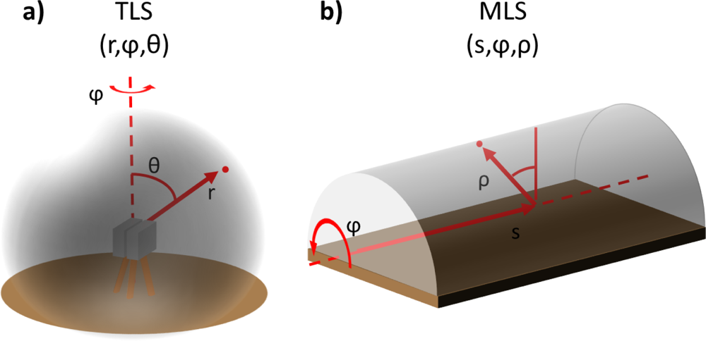
Figure 2.
Concepts of different sampling methods illustrated with a distance distribution of a synthetic laser point cloud. The blue area describes the distribution of the full dataset. The red and the green areas describe the subsample distributions when sampling sizes have been 20% and 50% of all points. Case (a) represents uniform point sampling (reference), case (b) represents leveled distance histogram sampling, and case (c) represents inversely weighted distance sampling (3D).
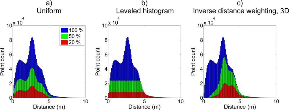
Figure 3.
(a) The point cloud of a single scanning location in Case Study I (the centre scan, Scan I). The number of points has been reduced down to 5% of the original for visualization purposes; (b) A point cloud distance histogram from the center of Scan I; (c) The normalized number of detected reference spheres with different sampling ratios. The full data (All) consisted of a total of 57 detected reference spheres; (d) The distance to the farthest detected reference sphere with different sampling ratios.
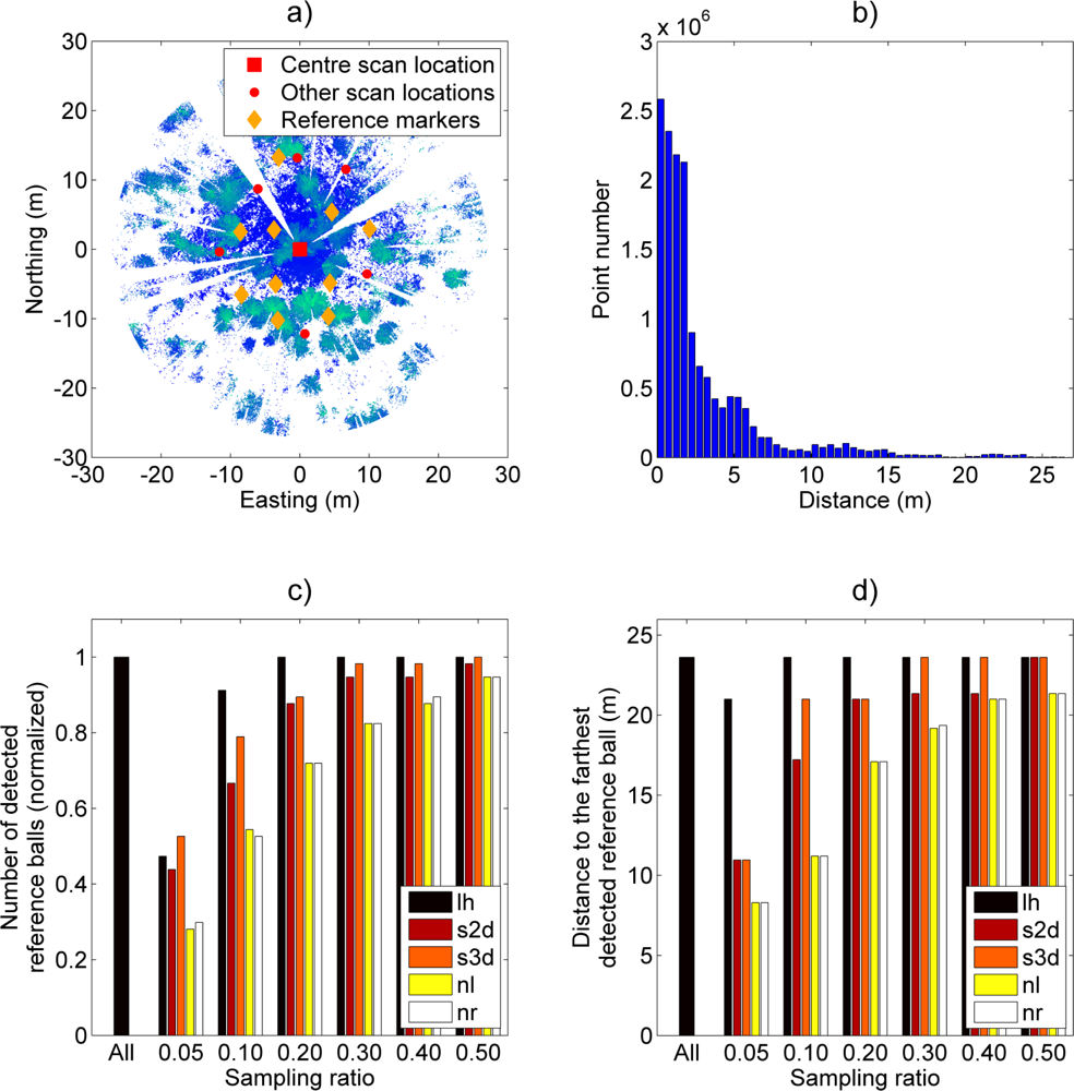
Figure 4.
(a) The test area in Case Study II. The trajectory of FGI Roamer is marked with green color. Manually detected reference poles are marked with red. The number of points (blue) has been reduced down to 10% of the original for visualization purposes. (b) Point cloud distance histogram (blue bars, left scale) and the reference target distribution (red bars, right scale). (c) Normalized sampling performance of different sampling techniques as a function of sampling ratio. Performance normalization was done against the results obtained with the full data. (d) Normalized total running time of the pole detection algorithm with different sampling methods as a function of sampling ratio. Normalization was done against the run time with the full data, which was 2,070 s.

Figure 5.
(a) The test area in Case Study III. The trajectory is drawn with green and wall points extracted from the full data are drawn with red. (b) Point cloud distance histogram. (c) Normalized sampling performance of different sampling techniques as a function of sampling ratio. The comparison is carried out by comparing the number of wall points in sampled point clouds against the results obtained with the full data. (d) Normalized total running time of the wall detection algorithm with different sampling methods as a function of sampling ratio. Normalization was done against the run time with the full data, which was 6,260 s.

Table 1.
Development of TLS and MLS systems over the last decade. All values are the maxima as reported in the reported reference(s). MLS systems that carry more than one scanner have their scanner number in parentheses. The Field Of View column (FOV) marked with an (L) means that a line scanner(s) was used. * Geovan MLS system used a Riegl LMS-Z210 scanner in its configuration.
| Year | Sensor | Type | Measurement Frequency (s−1) | Measurement Distance (m) | FOV (Hor × Ver, degs) | Reference |
|---|---|---|---|---|---|---|
| 1998 | Cyrax 2400 | TLS, Pulse | 8.0 × 10² | 50 | 40 × 40 | [13] |
| 2001 | VLMS | MLS, Pulse | (3×) 1.2 × 10⁴ | 50 | 0 × 300 (L) | [14] |
| 2002 | Z+f RI5003 | TLS, Phase | 6.3 × 10⁵ | 53 | 360 × 270 | [15,16] |
| 2003 | RIEGL LMS-Z420i | TLS, Pulse | 8.0 × 10³ | 800 | 360 × 80 | [17] |
| 2005 | Geovan * | MLS, Pulse | 2.0 × 10⁴ | 350 | 340 × 80 | [18,19] |
| 2006 | Faro LS880 | TLS, Phase | 1.2 × 10⁵ | 76 | 360 × 320 | [20] |
| 2010 | Optech Lynx M1 | MLS, Pulse | (2×) 5.0 × 10⁵ | 200 | 0 × 360 (L) | [21] |
| 2012 | Leica P20 | TLS, Pulse | 1.0 × 10⁶ | 120 | 360 × 270 | [22] |
| 2012 | Faro Focus 3D 120 | TLS, Phase | 9.8 × 10⁵ | 120 | 360 × 305 | [23] |
| 2009/13 | RIEGL VZ-400 | TLS, Pulse | 1.2 × 10⁵ | 600 | 360 × 100 | [24] |
Share and Cite
MDPI and ACS Style
Puttonen, E.; Lehtomäki, M.; Kaartinen, H.; Zhu, L.; Kukko, A.; Jaakkola, A. Improved Sampling for Terrestrial and Mobile Laser Scanner Point Cloud Data. Remote Sens. 2013, 5, 1754-1773. https://doi.org/10.3390/rs5041754
AMA Style
Puttonen E, Lehtomäki M, Kaartinen H, Zhu L, Kukko A, Jaakkola A. Improved Sampling for Terrestrial and Mobile Laser Scanner Point Cloud Data. Remote Sensing. 2013; 5(4):1754-1773. https://doi.org/10.3390/rs5041754
Chicago/Turabian StylePuttonen, Eetu, Matti Lehtomäki, Harri Kaartinen, Lingli Zhu, Antero Kukko, and Anttoni Jaakkola. 2013. "Improved Sampling for Terrestrial and Mobile Laser Scanner Point Cloud Data" Remote Sensing 5, no. 4: 1754-1773. https://doi.org/10.3390/rs5041754