Signal Classification of Submerged Aquatic Vegetation Based on the Hemispherical–Conical Reflectance Factor Spectrum Shape in the Yellow and Red Regions

 ,
,
Abstract
:1. Introduction
2. Materials and Methods
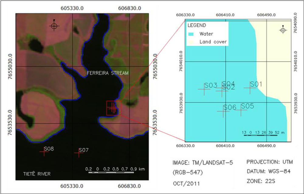
2.1. Study Area
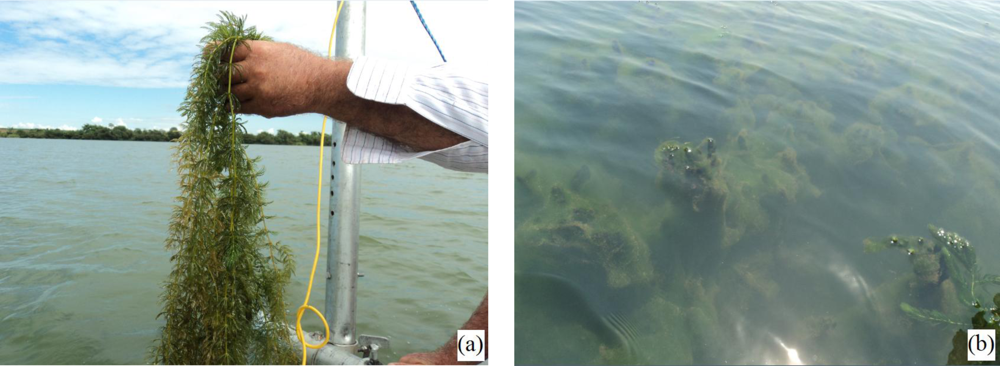
2.2. Field Survey
2.3. Data Analysis
2.3.1. Continuum-Removal Technique
2.3.2. Cluster Analysis
2.3.3. Spectral Angle Mapper (SAM)
3. Results and Discussion
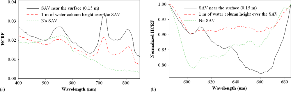
3.1. Continuum Removal
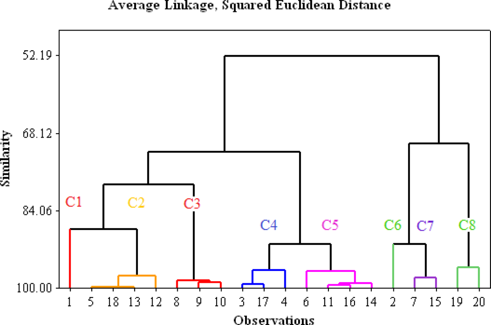
3.2. Cluster Analysis Classification
3.3. Spectral Angle Mapper (SAM)
4. Conclusions
Acknowledgments
References
- Esteves, F.A. Fundamentos de Limnologia, 2nd ed.; Interciência: Rio de Janeiro, Brazil, 1998. [Google Scholar]
- Wetzel, R.G. Limnology: Lake and River Ecosystems, 3rd ed.; Elsevier Academic Press: London, UK, 2001. [Google Scholar]
- Dekker, A.G.; Brando, V.E.; Anstee, J.M.; Pinnel, N.; Kutser, T.; Hoogeboom, E.J.; Peters, S.; Pasterkamp, R.; Vos, C.; Olbert, C.; Malthus, T.J.M. Imaging Spectrometry of Water. In Imaging Spectrometry: Basic Principles and Prospective Applications; van der Meer, F.D., Jong, S.M., Eds.; Kluwer Academic Publishers: New York, NY, USA, 2002; Chapter 11; pp. 307–359. [Google Scholar]
- Pitelli, R.L.C.M.; Toffaneli, C.M.; Vieira, E.A.; Pitelli, R.A.; Velini, E.D. Dynamics of the aquatic macrophyte community in the Santana reservoir in Pirai-RJ. Weed Sci 2008, 26, 473–480. [Google Scholar]
- Cavenaghi, A.L.; Velini, E.D.; Galo, M.L.B.T.; Carvalho, F.T.; Negrisoli, E.; Trindade, M.L.B.; Simionato, J.L.A. Caracterization of water quality and sediment related to the occurrence of aquatic plants in five Tietê waterhed reservoirs. Weed Sci 2003, 21, 43–52. [Google Scholar]
- Thomaz, S.M.; Souza, D.C.; Bini, L.M. Species richness and beta diversity of aquatic macrophytes in a large subtropical reservoir (Itaipu Reservoir. Brazil): The influence of limnology and morphometry. Hydrobiologia 2003, 505, 119–128. [Google Scholar]
- Bini, L.M.; Thomaz, S.M. Prediction of Egeria najas and Egeria densa occurrence in a large subtropical reservoir (Itaipu Reservoir. Brazil-Paraguay). Aquat. Bot 2005, 83, 227–238. [Google Scholar]
- Rybicki, N.B.; Carter, V. Light and temperature effects on the growth of wild celery and hydrilla. J. Aquat. Plant Manage 2002, 40, 92–99. [Google Scholar]
- Lee, K.H.; Lunetta, R.S. Wetland Detection Methods. In Wetland and Environment Applications of GIS; Lyon, J.G., McCarthy, J., Eds.; Lewis Publishers: New York, NY, USA, 1996; pp. 246–284. [Google Scholar]
- Adam, E.; Mutanga, O.; Rugege, D. Multispectral and hyperspectral remote sensig for identification and mapping of wetland vegetation: A review. Wetlands Ecol. Manag 2010, 18, 281–296. [Google Scholar]
- Ackleson, S.G.; Klemas, V. Remote sensing of submerged aquatic vegetation in lower Chesapeake Bay: A comparison of Landsat MSS to TM imagery. Remote Sens. Environ 1987, 22, 235–248. [Google Scholar]
- Peñuelas, J.; Gamon, J.A.; Griffin, K.L.; Field, C.B. Assessing community type, plant biomass, pigment composition, and photosynthetic efficiency of aquatic vegetation from spectral reflectance. Remote Sens. Environ 1993, 46, 110–118. [Google Scholar]
- Malthus, T.J.; George, D.G. Airborne remote sensing of macrophytes in Cefni Reservoir, Anglesey, UK. Aquat. Bot 1997, 58, 317–332. [Google Scholar]
- Han, L.; Rundquist, D.C. The spectral responses of Ceratophyllum demersum at varying depths in an experimental tank. Int. J. Remote Sens 2003, 24, 859–864. [Google Scholar]
- Hestir, E.L.; Khanna, S.; Andrew, M.E.; Santos, M.J.; Viers, J.H.; Greenberg, J.A.; Rajapakse, S.S.; Ustin, S.L. Identification of invasive vegetation using hyperspectral remote sensing in the California Delta ecosystem. Remote Sens. Environ 2008, 112, 4034–4047. [Google Scholar]
- Phinn, S.R.; Dekker, A.G.; Brando, V.E.; Roelfsema, C.M. Mapping water quality and substrate cover in optically complex coastal and reef waters: An integrated approach. Mar. Pollut. Bull 2005, 51, 459–469. [Google Scholar]
- Brando, V.E.; Anstee, J.M.; Wettle, M.; Dekker, A.G.; Phinn, S.R.; Roelfsema, C. A physics based retrieval and quality assessment of bathymetry from suboptimal hyperspectral data. Remote Sens. Environ 2009, 113, 755–770. [Google Scholar]
- Lyons, M.; Phinn, S.; Roelfsema, C. Integrating Quickbird multi-spectral satellite and field data: Mapping bathymetry, seagrass cover, seagrass species and change in Moreton Bay, Australia in 2004 and 2007. Remote Sens 2011, 3, 42–64. [Google Scholar]
- Hedley, J.D.; Roelfsema, C.M.; Phinn, S.R.; Mumby, P.J. Environmental and sensor limitations in optical remote sensing of coral reefs: Implications for monitoring and sensor design. Remote Sens 2012, 4, 271–302. [Google Scholar]
- Kirk, J.T.O. Light and Photosynthesis in Aquatic Ecosystems, 2nd ed.; Cambridge University Press: Cambridge, UK, 1994. [Google Scholar]
- Mobley, C.D. Light and Water: Radiative Transfer in Natural Waters; Academic Press: San Diego, CA, USA, 1994. [Google Scholar]
- Gitelson, A. The peak near 700 nm on radiance spectra of algae and water: Relationships of its magnitude and position with chlorophyll concentration. Int. J. Remote Sens 1992, 13, 3367–3373. [Google Scholar]
- Mittenzwey, K.-H.; Ullrich, S.; Gitelson, A.A.; Kondratiev, K.Y. Determination of chlorophyll a of inland waters on the basis of spectral reflectance. Limnol. Oceanogr 1992, 37, 147–149. [Google Scholar]
- Gitelson, A.; Garbuzov, G.; Szilagyi, F.; Mittenzwey, K-H.; Karnieli, A.; Kaiser, A. Quantitative remote sensing methods for real-time monitoring of inland waters quality. Int. J. Remote Sens 1993, 14, 1269–1295. [Google Scholar]
- Rundquist, D.C.; Han, L.H.; Schalles, J.F.; Peake, J.S. Remote measurement of algal chlorophyll in surface waters: The case for the first derivative of reflectance near 690 nm. Photogramm. Eng. Remote Sensing 1996, 62, 195–200. [Google Scholar]
- Goodin, D.G.; Han, L.; Fraser, R.N.; Rundquist, C.; Stebbins, W.A.; Schalles, J.F. Analysis of suspended solids in water using remotely sensed high resolution derivative spectra. Photogramm. Eng. Remote Sensing 1993, 59, 505–510. [Google Scholar]
- Chen, Z.; Curran, P.J.; Hansom, J.D. Derivative reflectance spectroscopy to estimate suspended sediment concentration. Remote Sens. Environ 1992, 40, 67–77. [Google Scholar]
- Han, L.; Rundquist, D.C.; Liu, L.L.; Fraser, R.N.; Schalles, J.F. The spectra responses of algal chlorophyll in water with varying levels of suspended sediment. Int. J. Remote Sens 1994, 15, 3707–3718. [Google Scholar]
- Han, L. Spectral reflectance with varying suspended sediment concentrations in clear and algae-laden waters. Photogramm. Eng. Remote Sensing 1997, 63, 701–705. [Google Scholar]
- Williams, D.J.; Rybicki, N.B.; Lombana, A.V.; O’brien, T.M.; Gomez, R.B. Preliminary investigation of submerged aquatic vegetation mapping using hyperspectral remote sensing. Environ. Monit. Assess 2003, 81, 383–392. [Google Scholar]
- Yuan, L.; Zhang, L. Mapping large-scale distribution of submerged aquatic vegetation coverage using remote sensing. Ecol. Inform 2008, 3, 245–251. [Google Scholar]
- Rotta, L.H.S. Inferência Especial Para Mapeamento de Macrófitas Submersas—Estudo de Caso.
- Clementson, L.A.; Parslow, J.S.; Turnbull, A.R.; McKenzie, D.C.; Rathbone, C.E. Optical properties of waters in Australasian sector of the Southern Ocean. J. Geophys. Res 2001, 106, 31611–31625. [Google Scholar]
- Brando, V.E.; Dekker, A.G. Satellite hyperspectral remote sensing for estimating estuarine and coastal water quality. IEEE Trans. Geosci. Remote Sens 2003, 41, 1378–1387. [Google Scholar]
- Lee, Z.; Casey, B.; Arnone, R.; Weidmann, A.; Parsons, R.; Montes, M.J.; Gao, B.C.; Goode, W.; Davis, C.O.; Dye, J. Water and bottom properties of a coastal environment derived from Hyperion data measured from the EO-1 spacecraft platform. J. Appl. Remote Sens 2007, 1, 1–16. [Google Scholar]
- Lee, Z.L.; Carder, K.L.; Mobley, C.D.; Steward, R.G.; Patch, J.S. Hyperspectral remote sensing for shallow waters: 2. Deriving bottom depths and water properties by optimization. Appl. Opt 1999, 38, 3831–3843. [Google Scholar]
- Casal, G.; Sánchez-Carnero, N.; Domínguez-Gómez, J.A.; Kutser, T.; Freire, J. Assessment of AHS (Airborne Hyperspectral Scanner) sensor to map macroalgal communities on the Ría de Vigo and Ría de Aldán coast (NW Spain). Mar. Biol 2012, 159, 1997–2013. [Google Scholar]
- Everitt, J.H.; Yang, C.; Escobar, D.E.; Webster, C.F.; Lonard, R.I.; Davis, M.R. Using remote sensing and spatial information technologies to detect and map two aquatic macrophytes. J. Aquat. Plant Manage 1999, 37, 71–80. [Google Scholar]
- Horler, D.N.H.; Dockray, M.; Barber, J. The red edge of plant leaf reflectance. Int. J. Remote Sens 1983, 4, 273–288. [Google Scholar]
- Curran, P.J.; Dungan, J.L.; Macler, B.A.; Plummer, S.E. The effect of a red leaf pigment on the relationship between red edge and chlorophyll concentration. Remote Sens. Environ 1991, 35, 69–76. [Google Scholar]
- Filella, I.; Peñuelas, J. The red edge position and shape as indicators of plant chlorophyll content. biomass and hydric status. Int. J. Remote Sens 1994, 15, 1459–1470. [Google Scholar]
- Gitelson, A.A.; Merzlyak, M.N. Remote estimation of chlorophyll content in higher plant leaves. Int. J. Remote Sens 1997, 18, 2691–2697. [Google Scholar]
- Knipling, E.B. Physical and physiological basis for the reflectance of visible and near-infrared radiation from vegetation. Remote Sens. Environ 1970, 1, 155–159. [Google Scholar]
- Elvidge, C.D.; Chen, Z. Comparison of broad-band and narrow red and near-infrared vegetation indices. Remote Sens. Environ 1995, 54, 38–48. [Google Scholar]
- Cho, H.J.; Kirui, P.; Natarajan, H. Test of muti-spectral vegetation index for floating and canopy-forming submerged vegetation. Int. J. Environ. Res. Publ. Health 2008, 5, 477–483. [Google Scholar]
- Han, L. Spectral Reflectance of Thalassia Testudinum with Varying Depths. Proceedings of 2002 IEEE International Geosciences and Remote Sensing Symposium (IGARSS’02), Toronto, ON, Canada, 24–28 June 2002; pp. 2123–2125.
- Analytical Spectral Devices Inc. FieldSpec® UV/VNIR: HandHeld Spectroradiometer User’s Guide; Analytical Spectral Devices Inc.: Boulder, CO, USA, 2002. [Google Scholar]
- Poli Control. Portable Digital/Bench Turbidimeter, Model AP 200 (0–1000 NTU), 2012. Available online: www.policontrol.com.br(accessed on 26 October 2012).
- BioSonics Inc. DT-X Digital Scientific Portable Echosounder. 2012. Available online: http://www.biosonicsinc.com/product-dtx-portable-echosounder.asp (accessed on 26 October 2012).
- Sabol, B.M.; Kannenberg, J.; Skogerboe, J.G. Integrating acoustic mapping into operational aquatic plant management a case study in Wisconsin. J. Aquat. Plant Manage 2009, 47, 44–52. [Google Scholar]
- Johnson, R.A.; Wichern, D.W. Applied Multivariate Statistical Analysis, 6th ed.; Pearson Education: Delhi, India, 2007. [Google Scholar]
- Clark, R.N.; Roush, T.L. Reflectance spectroscopy: Quantitative analysis techniques for remote sensing applications. J. Geophys. Res 1984, 89, 6329–6340. [Google Scholar]
- Kruse, F.A.; Lefkoff, A.B.; Boardman, J.W.; Heidebrecht, K.B.; Shapiro, A.T.; Barloon, P.J.; Goetz, A.F.H. The spectral image processing system (SIPS)—Interactive visualization and analysis of imaging spectrometer data. Remote Sens. Environ 1993, 44, 145–163. [Google Scholar]
- Kruse, F.A.; Lefkoff, A.B.; Dietz, J.B. Expert system-based mineral mapping in northern death valley. California/Nevada. using the Airbone Visible/Infrared Imaging Spectrometer (AVIRIS). Remote Sens. Environ 1993, 44, 309–336. [Google Scholar]
- Mutanga, O.; Skidmore, A.K.; Kumar, L.; Ferwerda, J. Estimating tropical pasture quality at canopy level using band depth analysis with continuum removal in the visible domain. Int. J. Remote Sens 2005, 26, 1093–1108. [Google Scholar]
- Youngentob, K.N.; Roberts, D.A.; Held, A.A.; Dennison, P.E.; Jia, X.; Lindernmayer, D.B. Mapping two Eucalyptus subgenera using multiple endmember spectral mixture analysis and continuum-removed imaging spectrometry data. Remote Sens. Environ 2011, 115, 1115–1128. [Google Scholar]
- Ge, S.; Carruthers, R.I.; Krammer, M.; Everitt, H.; Anderson, G.L. Multiple-level defoliation assessment with hyperspectral data: Integration of continuum-removed absorptions and red edges. Int. J. Remote Sens 2011, 32, 6407–6422. [Google Scholar]
- Carvalho, J.C.; Barbosa, C.C.; Novo, E.M.; Mantovani, J.E.; Melack, J.; Pereira Filho, W. Applications of Quantitative Analysis Techniques to Monitor Water Quality of Curuai Lake, Brazil. Proceedings of 2003 IEEE International Geosciences and Remote Sensing Symposium, (IGARSS’03), Toulouse, France, 21–25 July 2003; pp. 2362–2364.
- Krzanowski, W.J.; Marriott, F.H.C. Multivariate Analysis—Part 2: Classification Covariance Structure and Repeated Measurements; Arnold: London, UK, 1995. [Google Scholar]
- Minitab Inc. Software Minitab 15, 2006. Available online: www.minitab.com(accessed on 13 November 2012).
- Yuhas, R.H.; Goetz, A.F.H.; Boardman, J.W.; Green, R.O. Discrimination among Semi-Arid Landscape Endmembres Using the Spectral Angle Mapper (SAM) Algorithm. Proceedings of 3rd Annual JPL Airborne Geoscience Workshop, Pasadena, CA, USA, 1–5 June 1992; 1, pp. 147–149.
- Kruse, F.A.; Boardman, J.W.; Huntington, J.F. Comparison of airborne hyperspectral data and EO-1 Hyperion for mineral mapping. IEEE Trans. Geosci. Remote Sens 2003, 41, 1388–1400. [Google Scholar]
- Dennison, P.E.; Halligan, K.Q.; Roberts, D.A. A comparison of error metrics and constraints for multiple endmember spectral mixture analysis and spectral angle mapper. Remote Sens. Environ 2004, 93, 359–367. [Google Scholar]
- Yonezawa, C. Maximum likelihood classification combined with spectral angle mapper algorithm form high resolution satellite imagery. Int. J. Remote Sens 2007, 28, 3729–3737. [Google Scholar]
- Cho, M.A.; Debba, P.; Mathieu, R.; Naidoo, L.; Aardt, J.V.; Asner, G.P. Improving discrimination of Savanna tree species through a multiple-endmember spectral angle mapper approach: Canopy-level analysis. IEEE Trans. Geosci. Remote Sens 2010, 48, 4133–4142. [Google Scholar]
- Barbosa, C.C.F. Sensoriamento Remoto da Dinâmica da Circulação da Água no Sistema Planície de Curuai/Rio Amazonas. 2005; p. 281. [Google Scholar]
- MathWorks®. Software MatLab 7. Matlab®—The Language of Techinical Computing, 2004. Available online: www.mathworks.com(accessed on 13 November 2012).
- Han, L. Spectral reflectance with varying suspended sediment concentrations in clear and algae-laden waters. Photogramm. Eng. Remote Sensing 1997, 63, 701–705. [Google Scholar]
- Jensen, J.R. Remote Sensing of the Environment: An Earth Resource Perspective, 2nd ed.; Pearson Prentice Hall: Upper Saddle River, NJ, USA, 2007. [Google Scholar]


| Sites | Turbidity (NTU) | Channel | Samples | SAV | Water Column Height over the SAV (m) |
|---|---|---|---|---|---|
| S01 | 1.98 | Ferreira stream | 1 | NO | - |
| 2 | YES | 0.15 | |||
| 3 | YES | 0.01 | |||
| S02 | 1.31 | Ferreira stream | 4 | YES | 0.2 |
| 5 | YES | 2.0 | |||
| 6 | YES | 0.46 | |||
| 7 | YES | 0.07 | |||
| 8 | NO | - | |||
| S03 | 2.16 | Ferreira stream | 9 | NO | - |
| 10 | YES | 3.0 | |||
| 11 | YES | 0.63 | |||
| S04 | 1.67 | Ferreira stream | 12 | YES | 1.0 |
| 13 | YES | 0.22 | |||
| 14 | YES | 0.15 | |||
| S05 | 1.41 | Ferreira stream | 15 | YES | 0.3 |
| 16 | YES | 0.5 | |||
| 17 | YES | 0.05 | |||
| S06 | 1.45 | Ferreira stream | 18 | YES | 2.0 |
| S07 | 1.2 | Tietê River | 19 | NO | - |
| S08 | 1.2 | Tietê River | 20 | NO | - |
| T\R | 1 | 4 | 7 | 9 | 11 | 14 | 18 | 20 |
|---|---|---|---|---|---|---|---|---|
| 2 | 0.0428 | 0.0387 | 0.0122 | 0.0583 | 0.0318 | 0.031 | 0.0458 | 0.0752 |
| 3 | 0.0263 | 0.0265 | 0.014 | 0.0523 | 0.0176 | 0.0157 | 0.0377 | 0.0756 |
| 5 | 0.0166 | 0.0433 | 0.0355 | 0.0267 | 0.0168 | 0.0186 | 0.0127 | 0.0531 |
| 6 | 0.023 | 0.0326 | 0.0194 | 0.0427 | 0.0125 | 0.0128 | 0.0282 | 0.0658 |
| 8 | 0.0399 | 0.0717 | 0.0614 | 0.0071 | 0.0447 | 0.0466 | 0.019 | 0.0298 |
| 10 | 0.0253 | 0.0561 | 0.0492 | 0.0161 | 0.0299 | 0.032 | 0.0109 | 0.0432 |
| 12 | 0.0126 | 0.0383 | 0.0337 | 0.0326 | 0.0118 | 0.0135 | 0.0181 | 0.0598 |
| 13 | 0.0168 | 0.0303 | 0.0385 | 0.0455 | 0.0167 | 0.018 | 0.0333 | 0.0729 |
| 15 | 0.0281 | 0.0325 | 0.0143 | 0.0489 | 0.0186 | 0.0178 | 0.0349 | 0.0702 |
| 16 | 0.0131 | 0.0277 | 0.0305 | 0.0438 | 0.0085 | 0.0094 | 0.0297 | 0.0703 |
| 17 | 0.0284 | 0.0145 | 0.0193 | 0.0601 | 0.0195 | 0.0174 | 0.0453 | 0.0851 |
| 19 | 0.0785 | 0.1077 | 0.0905 | 0.0431 | 0.0809 | 0.0827 | 0.0557 | 0.0193 |
Share and Cite
Watanabe, F.S.Y.; Imai, N.N.; Alcântara, E.H.; Da Silva Rotta, L.H.; Utsumi, A.G. Signal Classification of Submerged Aquatic Vegetation Based on the Hemispherical–Conical Reflectance Factor Spectrum Shape in the Yellow and Red Regions. Remote Sens. 2013, 5, 1856-1874. https://doi.org/10.3390/rs5041856
Watanabe FSY, Imai NN, Alcântara EH, Da Silva Rotta LH, Utsumi AG. Signal Classification of Submerged Aquatic Vegetation Based on the Hemispherical–Conical Reflectance Factor Spectrum Shape in the Yellow and Red Regions. Remote Sensing. 2013; 5(4):1856-1874. https://doi.org/10.3390/rs5041856
Chicago/Turabian StyleWatanabe, Fernanda Sayuri Yoshino, Nilton Nobuhiro Imai, Enner Herenio Alcântara, Luiz Henrique Da Silva Rotta, and Alex Garcez Utsumi. 2013. "Signal Classification of Submerged Aquatic Vegetation Based on the Hemispherical–Conical Reflectance Factor Spectrum Shape in the Yellow and Red Regions" Remote Sensing 5, no. 4: 1856-1874. https://doi.org/10.3390/rs5041856