Impact of the Spatial Domain Size on the Performance of the T_s-VI Triangle Method in Terrestrial Evapotranspiration Estimation

Abstract

This study aims to investigate the impact of the spatial size of the study domain on the performance of the triangle method using progressively smaller domains and Moderate Resolution Imaging Spectroradiometer (MODIS) observations in the Heihe River basin located in the arid region of northwestern China. Data from 10 clear-sky days during the growing season from April to September 2009 were used. Results show that different dry/wet edges in the surface temperature-vegetation index space directly led to the deviation of evapotranspiration (ET) estimates due to the variation of the spatial domain size. The slope and the intercept of the limiting edges are dependent on the range and the maximum of surface temperature over the spatial domain. The difference of the limiting edges between different domain sizes has little impact on the spatial pattern of ET estimates, with the Pearson correlation coefficient ranging from 0.94 to 1.0 for the 10 pairs of ET estimates at different domain scales. However, it has a larger impact on the degree of discrepancies in ET estimates between different domain sizes, with the maximum of 66 W·m⁻². The largest deviation of ET estimates between different domain sizes was found at the beginning of the growing season.

1. Introduction

Evapotranspiration (ET) from the land surface is an important component in the surface energy balance and water balance. Accurate characterization of it is therefore very important in the study of the terrestrial ecosystem, climate dynamics and hydrologic cycle. At present, estimate of regional evapotranspiration has been made possible by using the remote sensing observations in combination with ancillary surface and atmospheric data. Since the 1980s, a number of satellite-based land surface flux models were developed to simulate surface-atmosphere interactions and to retrieve the terrestrial evapotranspiration over a wide range of spatial scales [1–7]. Among these models, the triangle model proposed by Jiang and Islam [4,8] is a direct estimation of evaporative fraction (EF: the ratio of ET to the available energy), based on the triangle shape formed by the scatter plot of remotely sensed vegetation index (VI) versus surface temperature (T_s) under a full range of vegetation cover and soil moisture availability within the study region. This model needs fewer assumptions and reduces the complexity of ET estimation over large heterogeneous areas [9,10].

A significant number of publications have demonstrated the reliability of this method in estimating regional ET [11,12]. However, large deviation from the ground-based measurements was also presented by [13,14]. Besides the effects of vegetation structure on the surface temperature, the neglect of local advection and the uncertainty in the Priestley–Taylor coefficient, the large deviation was also attributed to the incorrect determination of the dry edge and the wet edge in the T_s-VI triangle space [14]. The dry edge is the upper envelope of the T_s-VI space, pixels on which are taken as surfaces with the largest water stress for a range of VI. In contrast, the wet edge is the lower envelope of the T_s-VI space, pixels on which represent surfaces without water stress. Figure 1 shows the conceptual T_s-VI space. T_max,i and T_min,i are the corresponding maximum and minimum surface temperatures at the dry and wet edges, respectively for a given VI (see Figure 1).

The determination of the dry edge and the wet edge is a critical procedure in the triangle method in that they provide important boundary conditions of the contextual T_s-VI relationship. Based on the boundary conditions, EF for a pixel at a specific VI interval is deduced by weighting the extreme T_s values within the interval in terms of the T_s of the pixel (see Section 2). Therefore, the dry edge and wet edge determine EF for pixels within the two limiting edges and subsequently determine ET estimation.

Normally, the dry edge of the triangle method is derived from the remotely sensed T_s-VI scatter plot by a linear fit to data pairs of the maximum T_s values at each VI class interval (e.g., [12–15]). Surface albedo is helpful to constrain the dry edge when all surface conditions are not met within the study domain [16,17]. The wet edge is usually assumed to be a horizontal line and is determined by the T_s of the cold pixel with the largest VI value, the T_s of a water body or a well-irrigated agricultural field [4,18]. One requirement of the triangle method is that there are full ranges of soil moisture availability and vegetation cover within the study area. However, in actual practices, the number of pixels from a remote sensing image is usually insufficient to cover all kinds of soil wetness and vegetation fraction cover [19]. In this situation, large uncertainty and error from the improper selection of the limiting edges will occur. For instance, it is hard to find wet surface evaporating and transpiring at potential rates in arid and semi-arid areas. Likewise, for a study site where crops or vegetated areas are prevalent, the possibility of the presence of dry surface with negligible sensible heat flux in an image would be greatly reduced.

In addition, the triangle method assumes uniform atmospheric forcing within the study area. Meteorological forcing is also an important factor influencing surface temperature, as a result affects the determination of the dry/wet edge of the T_s-VI space. However, whether the assumption is met is rarely mentioned in literatures when the triangle method is applied. The great difficulty in retrieving regional and accurate data of air temperature may be a major reason for this.

In practice, satellite images with varying spatial coverage can be used to retrieve surface heat flux in the domain of interest. One would use a subset of an image specifically for a study site, taking the entire scene of the image, or even merge multiple scenes of images. Different images used in the calculation would result in different surface heat flux estimates because the corresponding geomorphological features may be different. Usually, increasing the domain size would increase the heterogeneity in the land surface and meteorological conditions, and result in variations in the boundary condition of the triangle method, consequently, influence ET estimates. Therefore, performance of the triangle method depends on the size of the domain being used. Additionally, the impact of spatial extent on the performance of the triangle method also depends on the methodology for estimating temperature endmembers.

The relationship between the domain size and the performance of the triangle method has been studied insufficiently. Chen [20] indicated that spatial extent has great effects on the relationship between T_s and VI. Long et al.[21] investigated the sensitivity of the Surface Energy Balance Algorithm for Land (SEBAL) to changes in domain size by applying SEBAL to sub-watersheds of different sizes and the entire Baiyangdian watershed in North China. They observed a root mean square deviation (RMSD) of 75 W·m⁻² in the sensible heat flux (H) estimates between different domain sizes. They concluded that the variation of surface temperature for the selected extremes (hot pixel and cold pixel) at different domain scales is a major reason for this. Long et al.[22] also indicated that the dry edge of the triangle method tends to move upward and the wet edge tends to move in the opposite direction as the domain is enlarged, which could result in a large deviation of EF estimates between different domain sizes. In fact, domain dependence of the triangle method is likely to be different especially when study areas have different physical and geomorphological features. The sites in Long’s studies are both located in humid or semi-humid area. Different from his studies, this study has a different focus by investigating how the triangle method is dependent on the domain size in arid area using more satellite images across the whole crop growing season. In addition, the underlying reasons for the moving of the limiting edges due to the variation of the domain size and the relationship between the ET estimates and the varying limiting edges were revealed quantitatively and extensively.

The objective of this study is to investigate the dependence of the T_s-VI triangle method on the domain size specifically for arid area. By applying the triangle method to five nested subareas of the Heihe River Basin in the arid northwestern China, five sets of ET estimates and the related evaluation matrix are compared. The new findings of this study would be helpful to optimize the size of domain when applying and improving the triangle method.

2. T_s-VI Triangle Method

The triangle method for ET estimation is based on the physical relationship between T_s and VI or vegetation fraction cover (F_r) [8].

The mathematical expression of latent heat flux (LE) is taken as follows (Jiang and Islam 1999):

$$LE=\varphi \left[\left(R_n-G\right)\frac{\mathrm{\Delta }}{\mathrm{\Delta }+\gamma }\right]$$

(1)

where ϕ represents a combined-effect parameter accounting for the aerodynamic resistance (dimensionless). R_n is the surface net radiation (W·m⁻²). G is the soil heat flux (W·m⁻²). Δ is the slope of saturated vapor pressure at the air temperature (KPa·C⁻¹). γ is the psychrometric constant (KPa·C⁻¹).

The value of ϕ for each of the pixels is derived through interpolation between upper and lower boundaries of ϕ for a specific interval of F_r (0 < F_r < 1). Assuming ϕ_min = 0 for the driest bare soil pixel and ϕ_max = 1.26 for the wet edge with the maximum F_r, global minimum and maximum ϕ can be conveniently determined. Jiang and Islam (1999) demonstrated that the upper bound of ϕ_max,i for each F_r is very close to 1.26. Given these two bounds, the value of ϕ for pixel i can be linearly interpolated based on the distance of the corresponding surface temperature to the two boundaries. F_r along the dry edge is used as the lower bound of ϕ_min,i. The ϕ_i for any pixel with a F_r and a surface temperature T_s, can be determined by

$${\varphi }_i=\frac{T_{\text{max},i}-T_{s,i}}{T_{\text{max},i}-T_{\text{min},i}}\left({\varphi }_{\text{max},i}-{\varphi }_{\text{min},i}\right)+{\varphi }_{\text{min},i}$$

(2)

where T_max,i and T_min,i are the corresponding maximum and minimum surface temperatures at the dry and wet edges, respectively for a given F_r (see Figure 1).

In this study, R_n and G were obtained following the equations by Zhang et al. [19]:

$$R_n=S_0\left(1-\alpha \right)+R_{ld}-\sigma \epsilon T_s^4$$

(3)

$$R_{ld}=\sigma T_a^4\left[1-0.261\text{exp}\left(-0.000777{\left(273-T_a\right)}^2\right)\right],$$

(4)

$$G\approx 0.3\left(1-0.9F_r\right)R_n$$

(5)

where the item of R_ld is the downward longwave radiation and is estimated by the method proposed by Idso and Jackson [23], σ is the Stefan–Boltzmann constant, T_a is the air temperature, S₀ is the solar shortwave radiation, α is the surface albedo and T_s is the surface temperature, ε is calculated by a weighting average of soil/vegetation emissivities (ε_s, ε_v) according to their proportion in a pixel (Equation (6)). ε_s = 0.96 and ε_v = 0.98 are used in the calculation. F_r is estimated from the normalized difference vegetation index (NDVI) [24]:

$$\epsilon =F_r{\epsilon }_v+\left(1-F_r\right){\epsilon }_s$$

(6)

An automatic edge determination algorithm presented by Tang et al. [12] was used to find the dry edge in the study. This algorithm can automatically filter the spurious dry points and is more robustly resistant to the outliers. As for the horizontal wet edge, the lowest T_s value at dense vegetation cover was selected as the constant temperature at the wet edge. If pixels show relatively low T_s values but not high NDVI values, it implies an absence of dense vegetation cover, generally occurring in the early stage of crop growing season. In this case, quality control data from the land surface temperature product of MODIS was used to exclude pixels that have uncertainties of 3 k in T_s retrievals. Then, the pixel with the lowest T_s value was taken as the temperature at the wet edge.

3. Study Site and Data

3.1. Area Description

Our study area is the Heihe River Basin in the arid northwestern China, ranging in latitude between 37.75°N and 42.67°N and in longitude between 96.07°E and 102.07°E (Figure 2). The Heihe River, the second largest inland river in China, is 821 km long with a basin of 134,000 km², rising in the Qilian Mountain and flowing northward through 11 counties in 3 Provinces to become the East and the West of Juyan Lakes.

The basin comprises three major geomorphologic divisions from the south to the north, namely, the southern Qilian Mountains (the upper reach), the middle Hexi Corridor (the middle reach) and the northern Alxa High-plain (the lower reach). Elevations decrease from the south to the north, ranging from around 5,100 m to 500 m (Figure 2). Land cover ranges from woodland and grassland in the southern mountainous areas to cropland over the middle reach and to bare land in the lower plain (Figure 3). Bare land indicates the Gobi desert, saline and alkaline land and bare soil. Mean annual precipitation is about 500 mm, 200 mm and 42 mm for the upper, the middle and the lower reaches, respectively.

To investigate the relationship between the domain size and the triangle model performance, five different spatial domains were set up. The five domains include the entire basin (Domain I in Figure 3) and the four subareas of the basin, which are the area covering the middle Hexi Corridor and the Alxa High-plain (Domain II in Figure 3), the area covering the middle Hexi Corridor (Domain III in Figure 3), the area covering Zhangye, Linze and Gaotai (Domain IV in Figure 3) and the area covering only Zhangye (Domain V in Figure 3). The five domains are progressively decreasing and Zhangye is the overlapping area among all the five domains. Gobi desert in Ejina and Jinta represents the driest conditions in the basin. A minuscule amount of rain less than 50 mm per year [25] is the major reason for this. From the perspective of rainfall, Domain I and II have the drier surface conditions compared with the other three subareas. The highest heterogeneity of landscape and elevation is seen in Domain I because increasing the domain size would generally encompass more diverse land cover types, atmospheric forcing and more complex topography. Large difference between different domain sizes would help to clarify the question about the impact of the spatial domain size on the performance of the triangle method.

3.2. Moderate Resolution Imaging Spectroradiometer (MODIS) Data

Data of the daytime surface temperature (LST_Day_1 km), the overpass-time (Day_view_time), 16-day Normalized Difference Vegetation Index (1_km_16_days_NDVI) and 8-day Albedo (Albedo_BSA_Band_shortwave) extracted respectively from the MODIS products of land surface temperature (MOD11A1), 16-day Vegetation Indices (MOD13A2) and 8-day Albedo (MCD43B3) were used as the inputs for the triangle method. All the data were georeferenced and were re-sampled to 1 km spatial resolution with the MODIS Reprojection Tool (MRT). Because T_s-VI triangle space can not be constructed during non-growing seasons when there is almost no green vegetation in the basin except the needle-leaved evergreen forest in Qilian Mountains, only the clear-sky MODIS data in 2009 during the growing season from April to September were used. Because only one image is available every 16 days for MODIS NDVI product, data of surface temperature and Albedo matching closest with the date of the NDVI data were used to estimate ET. MOD11A1 quality information was used to exclude MODIS data having large uncertainties in surface temperature retrievals. After screening, days in which valid data can cover 90% of the whole Heihe Revier Basin were kept. Finally, 10 clear-sky days during the growing season from April to September in 2009 were used to investigate the impact of the spatial domain size on the performance of the Ts-VI triangle method in terrestrial evapotranspiration estimation.

3.3. Meteorological Data

As shown in Equations (1)–(5), solar radiation (S₀) and air temperature (T_a) are required to calculate R_n and Δ. In this study, meteorological data of S₀ and T_a from the Global Data Assimilation System (GDAS); the global meteorological weather forecast model of the National Centers for Environmental Prediction [26] were used, with 6 hourly (00, 06, 12, 18 UTC), global, 50 km resolution. A bilinear interpolation method was used to expand data of S₀ and T_a to a 1 km resolution, which uses 4 neighboring points to compute the interpolation weights. A linear interpolation method was used to get S₀ and T_a at overpass time of MODIS (about 03 UTC at the Heihe River Basin), which computes the temporal weights based on data at 00 and 06 UTC.

4. Results

4.1. Comparisons of Dry/Wet Edges Among Different Domain Sizes

Based on the T_s and F_r images covering Domain I, II, III, IV and V, respectively, we obtained five sets of dry/wet edges for each of the 10 days.

Table 1. Statistics of the determined dry/wet edges, the maximum surface temperature (T_s_max) over the subarea for 10 clear-sky days.

a (K)						b
DOY	I	II	III	IV	V	I	II	III	IV	V
96	315.9	316.0	315.7	311.1	310.9	−32.7	−32.5	−31.8	−5.6	−5.2
112	322.1	321.9	321.3	315.9	313.7	−30.4	−31.2	−28.8	−9.9	−7.7
121	323.0	320.1	320.2	315.8	310.8	−25.6	−20.6	−20.7	−18.6	−13.0
144	327.3	327.5	326.5	325.7	322.4	−25.7	−26.4	−24.2	−21.7	−18.4
152	331.3	331.3	330.9	328.2	320.1	−33.9	−33.9	−33.6	−29.1	−17.7
163	331.4	331.5	329.3	327.8	322.5	−30.2	−30.8	−27.4	−22.0	−16.8
176	332.9	333.1	331.6	330.8	328.2	−26.1	−26.7	−24.2	−23.5	−20.7
192	334.1	333.5	331.7	330.7	324.5	−31.6	−28.4	−28.3	−25.9	−18.7
224	333.6	332.1	331.4	330.9	329.4	−29.8	−24.3	−24.1	−24.8	−23.8
231	328.8	329.3	326.3	317.1	308.9	−30.3	−30.1	−30.1	−19.4	−8.9

Table 1. Statistics of the determined dry/wet edges, the maximum surface temperature (T_s_max) over the subarea for 10 clear-sky days.

c (K)						Ts_max(K)
DOY	I	II	III	IV	V	I	II	III	IV	V
96	283.2	283.5	283.9	304.1	304.6	316.9	316.9	314.3	314.3	314.3
112	291.6	290.8	292.5	306.0	306.1	321.3	321.3	319.4	319.1	315.1
121	292.4	291.7	291.9	297.2	297.9	318.9	318.9	318.9	318.7	312.5
144	298.3	300.8	301.6	302.3	302.3	329.6	329.6	326.7	326.1	323.8
152	291.9	293.1	292.7	295.9	297.2	328.2	328.2	327.7	327.0	322.9
163	294.2	294.9	294.9	300.8	300.6	330.9	330.9	329.7	329.7	324.3
176	297.7	300.3	300.6	306.6	306.7	334.5	334.5	331.8	331.8	331.8
192	294.6	296.6	296.8	303.0	302.6	333.8	333.8	332.0	331.8	326.0
224	293.1	295.9	296.4	305.3	305.4	336.5	336.5	331.0	330.8	328.9
231	291.4	291.2	291.3	297.6	299.4	329.5	329.5	323.5	323.5	312.7

a and b respectively represents the intercept and the slope of the dry edge

c represents the constant temperature at the wet edge and also represents the minimum surface temperature

shows the statistics of the determined dry/wet edges and the maximum surface temperatures (T_s_max) over each area for each day.

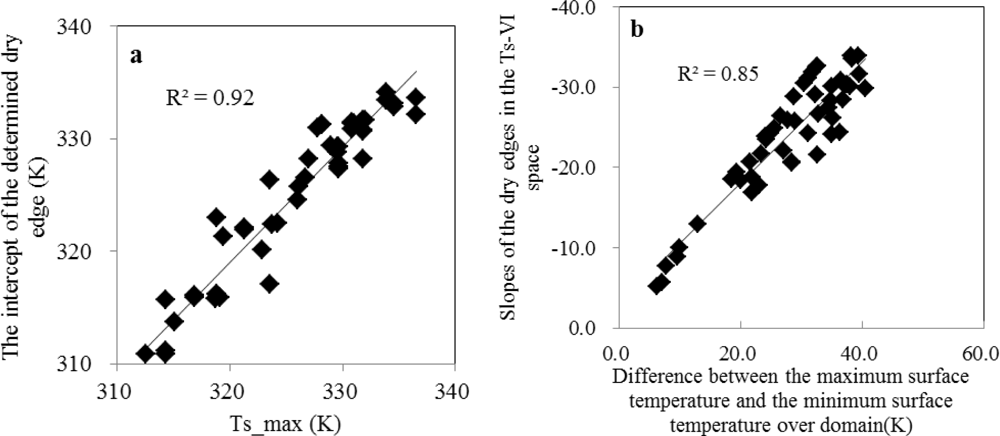
In general, a slight difference of the intercepts of dry edge for Domain I, II and III was found. Compared with the intercepts for Domain IV and V, Domain I, II and III have much higher values. This phenomenon can be related to T_s_max corresponding to the five areas. Figure 4(a) illustrates the relationship between the intercept of the determined dry edge and T_s_max for the five areas for the 10 days. It displays a very good correlation coefficient (R²), indicating high surface temperature of bare soil usually could lead to high intercepts of the dry edge. 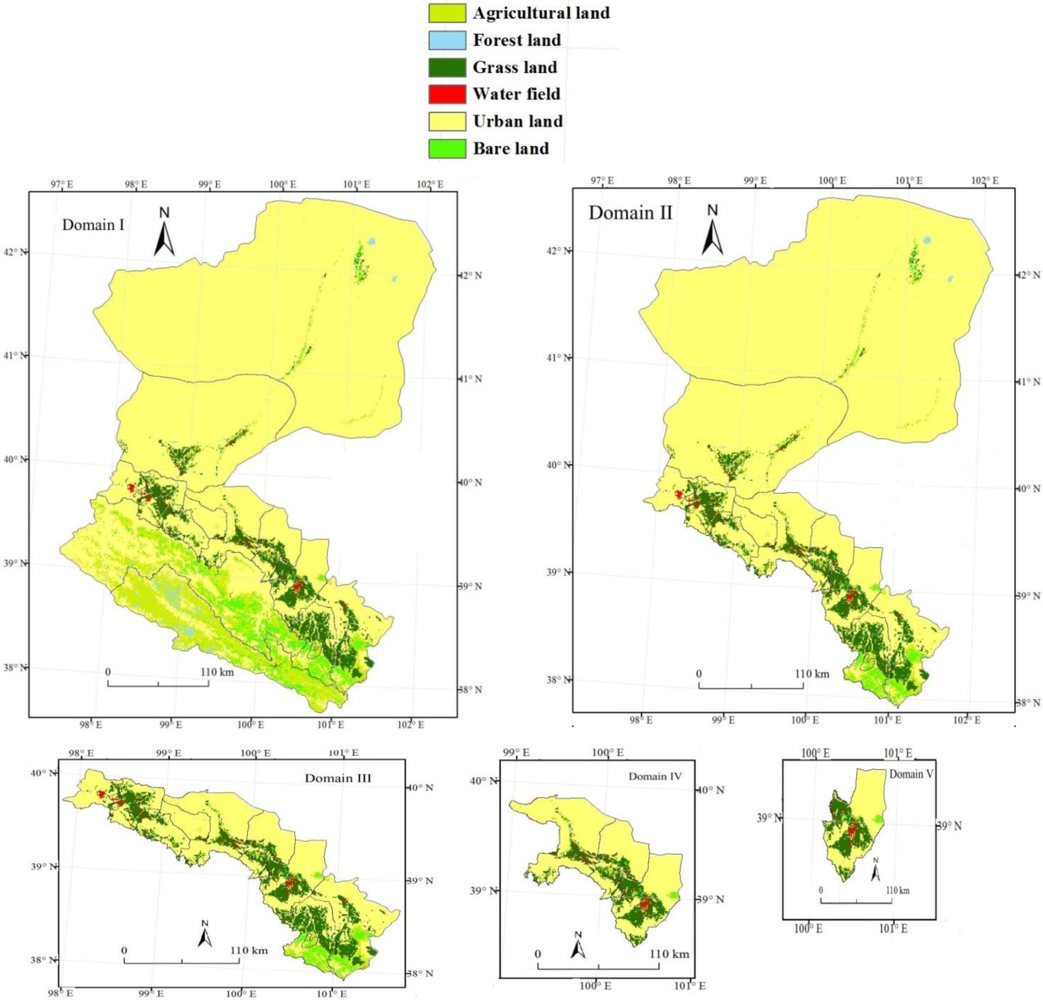Table 1 also shows T_s_max are the highest for Domain I and II, followed in turn by Domain III, IV and V. As mentioned in Section 3.1, Gobi desert in Ejina and Jinta is the driest surface in the basin and therefore produced the highest T_s_max for Domain I and II. Comparatively, the absence of extremely dry surface in Domain V results in the lowest intercept of the dry edge.

In addition, it can be seen from Table 1 that the slopes of the dry edges for Domain I, II and III are quite different from those for Domain IV and V, especially for Domain V. The slopes for Domain I, II and III are obvious steeper than that for Domain IV and V, which means that the decrease of surface temperature due to the increase of F_r happens much faster for Domain I, II and III. As mentioned in Section 2, the slope of the dry edge is determined by a linear regression between the maximum surface temperatures and the corresponding F_r interval. In the case where there is a wide range of maximum surface temperature for a range of F_r resulting from the combined effect of soil moisture, elevation, land use type, a steep slope of the dry edge would be produced. Generally speaking, the larger the domain size is, the more heterogeneous land surface is and thereby the steeper the slope of the dry edge is. The difference between T_s_max and the minimum surface temperature (c in Table 1) over the domain could represent the heterogeneity of land surface to a certain degree and was correlated with the slopes of the dry edges, as shown in Figure 4(b). A good linear relationship was observed. It could be concluded that when enlarging the domain size, the slope of the dry edge tends to be steeper. When the extremely dry or wet surfaces are not available, the slope of the dry edge tends to be gentler.

The largest differences in slopes of the five domains were observed on DOY (day of year) 96, and 112. It is up to 27.5 K, 22.7 K between Domain I and V, respectively for the two days. The growing season of the dominant crops (maize and spring wheat) in the basin is from April to September. DOY 96 and 112 are at the early stage of the growing season. An absence of densely vegetated surfaces in Domain IV and V during the early stage of the crop growing season leads to a higher temperature for wet surfaces (see c value in Table 1) by contrast with Domain I, II and III. This produces a narrower range of T_s on DOY 96 and 112, and therefore produces the gentler slopes. Values of (a–c) for Domain V for the two days are only 6.3 K and 7.6 K, while values of (a–c) are more than 20 K for the days in the middle of the growing season. The results indicate that the slope of the dry edge in T_s-VI space would be obviously overestimated during the early stage of crop growth or for the domain with no full vegetation cover. For Domain I, II and III, low surface temperatures of forest and grass land at high altitudes (Figure 2–3) contribute to the lower c values and thereby produce the larger (a–c) values and steeper slopes.

Similar to the largest difference of the slopes for the upper boundaries, the largest contrast in the lower boundaries were also observed between Domain I and V. On DOY 96 and 112, the differences of c values between Domain I and V are as large as 15∼20 K. This is consistent with the above description of the absence of extremely wet surface for Domain V at the beginning of the growing season.

4.2. Variation in ET Estimates with Domain Size

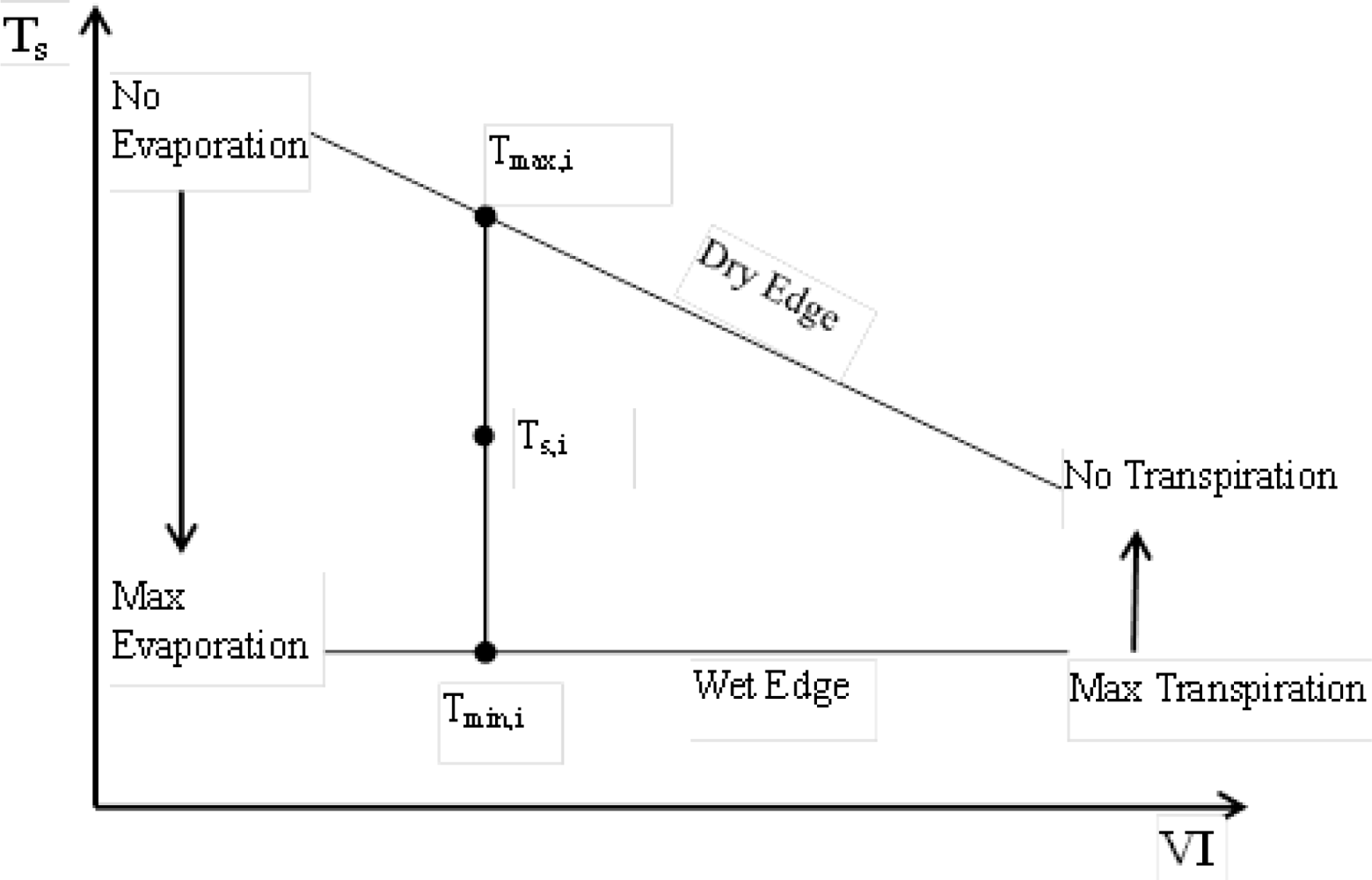
ET estimates from the triangle method is substantially dependent on the boundaries in the T_s-VI space via the ϕ estimates from T_max,i and T_min,i using Equations (1)–(2). ET estimates from the domains that have an overlapping area were compared. For example, Domain V was compared with Domain I, II, III and IV. ET estimates of Domain IV were compared with that of Domain I, II and III, and so it is with ET estimates of Domain III and II.

Table 2. The average of the Pearson correlation coefficient (r), Root Mean Square Difference (RMSD, W·m⁻²) and Mean of Difference (MD, W·m⁻²) of the 10 pairs of ET estimates over the 10 days (a) Domain V; (b) Domain IV; (c) Domain III; (d) Domain II).

a	r				RMSD				MD
DOY	I–V	II–V	III–V	IV–V	I–V	II–V	III–V	IV–V	I–V	II–V	III–V	IV–V
96	0.9935	0.9933	0.9940	1.0000	65.89	65.44	65.65	6.98	−46.68	−46.06	−46.54	−4.11
112	0.9857	0.9862	0.9878	0.9983	42.37	43.94	42,16	15.75	−20.43	−22.64	−21.01	12.38
121	0.9816	0.9888	0.9888	0.9941	25.40	22.80	22.53	15.29	−18.01	−11.46	−10.99	9.41
144	0.9881	0.9984	0.9989	0.9989	12.85	14.42	13.31	13.35	−3.41	12.06	11.93	12.79
152	0.9970	0.9975	0.9975	0.9985	26.83	28.34	26.98	26.04	20.78	23.17	21.43	23.25
163	0.9959	0.9971	0.9967	0.9993	22.86	23.26	19.56	20.89	7.64	8.84	4.72	18.85
176	0.9956	0.9975	0.9973	0.9998	19.78	17.79	16.10	10.32	−7.64	−2.94	−5.53	8.71
192	0.9972	0.9976	0.9983	0.9996	25.88	24.67	21.89	24.65	7.29	11.49	6.23	21.57
224	0.9964	0.9965	0.9969	0.9999	17.23	13.33	13.63	4.32	−9.77	−7.59	−8.78	3.69
231	0.9400	0.9378	0.9489	0.9891	38.63	38.67	38.87	28.71	0.84	1.53	−5.41	5.79
average	0.9871	0.9891	0.9905	0.9977	29.77	29.27	28.07	16.63	−6.94	−3.36	−5.40	11.23

Table 2. The average of the Pearson correlation coefficient (r), Root Mean Square Difference (RMSD, W·m⁻²) and Mean of Difference (MD, W·m⁻²) of the 10 pairs of ET estimates over the 10 days (a) Domain V; (b) Domain IV; (c) Domain III; (d) Domain II).

b	r			RMSD			MD
DOY	I–IV	II–IV	III–IV	I–IV	II–IV	III–IV	I–IV	II–IV	III–IV
96	0.9928	0.9926	0.9935	54.95	54.50	54.81	−42.28	−41.73	−42.24
112	0.9890	0.9895	0.9909	32.40	33.96	32.51	−19.24	−21.15	−20.14
121	0.9910	0.9991	0.9992	19.04	16.14	15.78	−19.14	−13.46	−13.04
144	0.9927	0.9997	0.9999	15.84	4.59	2.36	−13.22	1.38	0.23
152	0.9993	0.9996	0.9995	5.56	5.68	5.03	1.37	3.26	1.59
163	0.9979	0.9986	0.9984	13.60	13.16	13.50	−4.25	−3.10	−8.63
176	0.9961	0.9979	0.9978	17.56	13.91	14.58	−11.49	−6.95	−10.71
192	0.9980	0.9982	0.9988	14.67	10.82	13.89	−7.70	−4.91	−10.68
224	0.9971	0.9973	0.9975	14.57	11.89	12.63	−9.88	−8.94	−10.16
231	0.9816	0.9808	0.9861	21.14	21.58	18.71	9.00	9.65	2.65
average	0.9936	0.9953	0.9962	20.93	18.62	18.38	−11.68	−8.59	−11.11

Table 2. The average of the Pearson correlation coefficient (r), Root Mean Square Difference (RMSD, W·m⁻²) and Mean of Difference (MD, W·m⁻²) of the 10 pairs of ET estimates over the 10 days (a) Domain V; (b) Domain IV; (c) Domain III; (d) Domain II).

c	r		RMSD		MD		d	r	RMSD	MD
DOY	I–III	II–III	I–III	II–III	I–III	II–III	DOY	I–II	I–II	I–II
96	1.0000	1.0000	0.68	0.54	−0.37	0.32	96	1.0000	0.64	−0.63
112	0.9999	1.0000	1.46	2.73	0.33	−1.70	112	1.0000	2.04	1.96
121	0.9919	1.0000	1.14	0.44	−1.03	−0.43	121	0.9867	2.65	−1.53
144	0.9899	0.9998	3.34	2.66	−1.12	0.49	144	0.9930	2.92	−2.11
152	1.0000	1.0000	1.86	1.82	−0.89	1.78	152	0.9999	2.48	−2.15
163	0.9999	0.9999	4.93	5.78	3.37	4.91	163	0.9999	2.01	−1.75
176	0.9996	0.9999	4.98	4.14	−1.89	3.16	176	0.9994	5.79	−5.32
192	,0.9997	0.9998	5.53	5.30	0.80	4.72	192	0.9999	2.85	−1.30
224	0.9996	0.9999	4.83	1.36	−1.23	0.77	224	0.9995	2.94	0.67
231	0.9994	0.9991	6.36	7.14	5.75	6.27	231	1.0000	1.21	−1.12
average	0.9980	0.9998	3.51	3.19	0.37	2.03	average	0.9978	2.55	−1.33

shows the statistics of the 10 pairs of ET estimates. For ET estimates of Domain V (Table 2(a)), the smallest differences were observed between Domain IV and V, with an average RMSD of 16 W·m⁻² for the 10 days. The largest differences were found between Domain I and V, yielding an RMSD of 29 W·m⁻² for the 10-day average. This is consistent with the smallest difference in the limiting edges between Domain IV and V and the largest difference between Domain I and V (Table 1). The comparison results among Domain I versus V, II versus V and III versus V were very similar for the 10 days, which can be attributed to the similar dry/wet edges between them. When compared with the results at the beginning (DOY 96 and 112) of growing season for Domain I versus V, II versus V and III versus V, the RMSD values in the middle of growing season were obvious lower. The maximum RMSD was identified for Domain I versus V on DOY 96, with an RMSD of 66 W·m⁻². This can be explained by the larger difference of the dry/wet edges for the domains in the early stage of growing season and the smaller difference in the middle stage of growing season.

For the ET estimates in Domain IV (Table 2(b)), the largest RMSD was found between Domain I and IV, with a ten-day average of 21 W·m⁻². Similar to the comparison of ET estimates for Domain V, the RMSD of ET estimates between Domain IV and the other three Domain I, II, III are also significantly higher at the beginning of growing season than in the middle, which is as high as 55 W·m⁻² on DOY 96.

When comparing the ET estimates for Domain II and III (Table 2(c,d)), it gives much smaller RMSD than the prior comparisons. And the previously observed phenomenon of larger RMSD occurring at the beginning of growing season disappeared. This may be due to the similar limiting conditions among Domain I, II and III.

The trend of ET estimates with increasing domain size was not completely reflected from the mean difference of ET estimates between the five domain sizes. Some days exhibit positive values, while some days exhibit negative values.

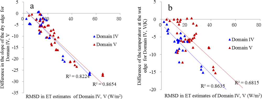
The above results indicate that the difference of the dry/wet edges in the T_s-VI space may be a key contributor to the difference of ET estimates for domains with different sizes. Figure 5 quantitatively illustrates the relationship between the difference of ET estimates of Domain IV and Domain V at different domain scales and the difference of the boundary conditions of the T_s-VI space. Apparently, differences in the slopes of the dry edges of the T_s-VI space (difference of b value in Table 1) between Domain IV and Domain I, II, III are linearly correlated with the RMSD of ET estimates between them. Good linear correlation was also found between the differences of b values and the RMSD of ET estimates (Table 2(a)) between Domain V and the other four domains. From Figure 5(b), difference of the constant temperatures at the wet edges (difference of c value in Table 1) is generally proportional to the values of RMSD of ET estimates between Domain IV and Domain I, II, III. So is the relationship for the differences of c values and the RMSD of ET estimates between Domain V and the other four domains. However, no linear relationship was found for ET estimates of Domain III and Domain II, which was not displayed in the paper. This is primarily because the dry/wet edges for Domain I, II and III are too similar to find significant differences. Overall, the dependence of the triangle method on the domain size is mostly originated from the dependence of the limiting edges on domain size.

Additionally, the average Pearson correlation coefficients (r) above 0.98 were found for each pair of ET estimates. This indicates that the difference of the determined limiting edges for different domain sizes has little impact on the spatial pattern of ET estimates. Even for the pair of Domain I and V, which has the largest contrast of the limiting edges, a high r value of 0.987 was obtained.

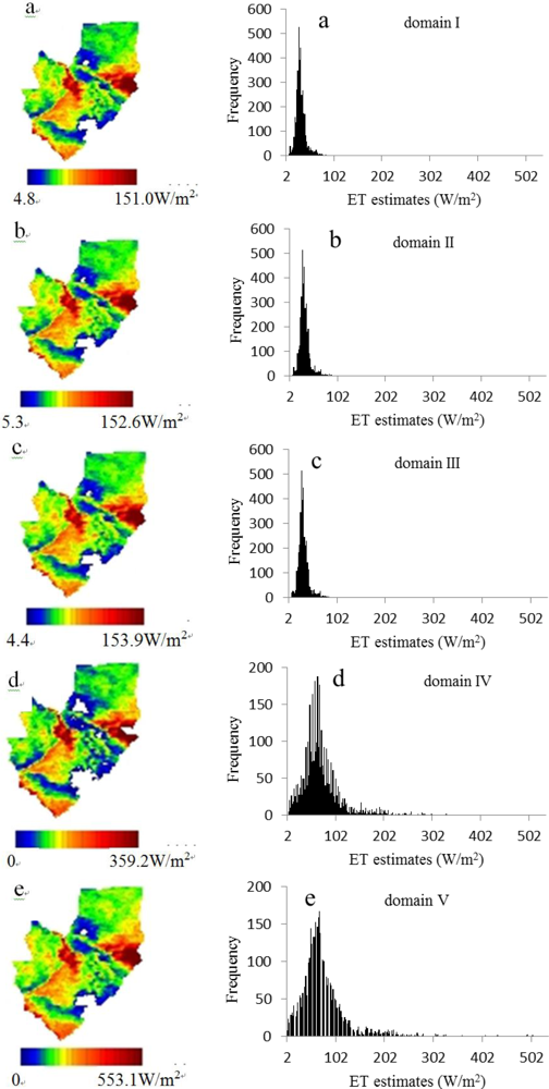
Figure 6 illustrates the five maps and the frequency histograms of ET estimates over the common overlapping Domain V on DOY 96 when the difference of ET estimates between different domain sizes are the largest. Similar distribution patterns were observed between the five sets of ET estimates, with higher ET in agricultural land and lower ET in bare land. It seems that the change of the limiting edges in T_s-VI space with domain size does not influence the spatial pattern of ET estimates. However, there are large differences in the magnitude of ET estimates between different domain sizes in terms of their histograms. Results explicitly revealed that ET estimates from Domain IV, V are much larger than that from Domain I, II and III on DOY 96, showing the areal mean of ET estimates of 72 W·m⁻², 76 W·m⁻², 32 W·m⁻², 33 W·m⁻² and 32 W·m⁻², respectively for Domain IV, V, I, II and III.

5. Conclusions

To investigate how domain size influences the performance of the triangle method, the method was applied to five nested subareas of the Heihe River basin in arid northwestern China where large variations of land cover, vegetation fractional cover, surface temperature and altitude are found between the five subareas. The impact of spatial extent on the performance of the triangle method resulting from the variability of soil moisture and vegetation cover at the sensor resolution was specially discussed. By comparing the determined dry/wet edges and ET retrievals between the five subareas, the relationship between the triangle method and the domain size is quantitatively investigated.

Results show that: (1) the intercept of the dry edge in the T_s-VI space is determined largely by the highest surface temperature in the spatial domain. In the case that the extremely dry surface is absent in the spatial domain, the intercept of the dry edge would be underestimated. In the study, it was underestimated by 20 K on DOY 231. As the domain size is increased, the extreme high surface temperature tends to increase and the extreme low surface temperature tends to decrease. (2) a large range of surface temperature in the spatial domain could lead to a steep slope of the determined dry edge. With the increase of the domain size, the slope of the dry edge tends to be steeper because of the increasing diversity of land surface types. When the extremely dry and wet surfaces are absent, the slope of the dry edge tends to be gentler. The maximum difference of the slopes of the dry edges between different domain sizes is up to 27 in the study. (3) large differences of the limiting edges between different domain size tend to arise in the beginning of the growing season. Because densely vegetated surfaces with low surface temperature are often absent during that time, the range of surface temperature is greatly reduced at a small domain, producing gentler slopes of the dry edge. (4) ET estimates from the triangle method depend on the domain size owing to the domain dependence of the limiting edges of the T_s-VI space. The degree of discrepancies in ET estimates between different domain sizes corresponds to the degree of discrepancies in the limiting edges between different domain sizes. The maximum difference of ET estimates of 66 W·m⁻² between different domain sizes was produced in the study. (5) the Pearson correlation coefficients for ET estimates at different domain scales are as high as 0.99. This indicates that the difference of the determined limiting edges between different domain sizes has little impact on the spatial pattern of ET estimates.

References

1. Norman, J.M.; Kustas, W.P.; Humes, K.S. A two-source approach for estimating soil and vegetation energy fluxes from observation of directional radiometric surface temperature. Agric. For. Meteorol 1995, 77, 263–293. [Google Scholar]
2. Bastiaanssen, W.G.M.; Menenti, M.; Feddes, R.A.; Holtslag, A.A.M. A remote sensing surface energy balance algorithm for land (SEBAL) 1. Formulation. J. Hydrol 1998, 213, 198–212. [Google Scholar]
3. Kustas, W.P.; Norman, J.M. Evaluation of soil and vegetation heat flux predictions using a simple two-source model with radiometric temperatures for partial canopy cover. Agric. For. Meteorol 1999, 94, 13–29. [Google Scholar]
4. Jiang, L.; Islam, S. Estimation of surface evaporation map over southern Great Plains using remote sensing data. Water Resour. Res 2001, 37, 329–340. [Google Scholar]
5. Su, Z.B. The surface energy balance system (SEBS) for estimation of turbulent heat fluxes. Hydrol. Earth Syst. Sci 2002, 6, 85–89. [Google Scholar]
6. Zhang, R.H.; Sun, X.M.; Wang, W.M.; Xu, J.P.; Zhu, Z.L.; Tian, J. An operational two-layer remote sensing model to estimate surface flux in regional scale: Physical background. Sci. China Ser. D 2005, 48, 225–244. [Google Scholar]
7. Allen, R.G.; Tasumi, M.; Trezza, R. Satellite-based energy balance for Mapping Evapotranspiration with Internalized Calibration (METRIC)-model. J. Irrig. Drain Eng 2007, 133, 380–394. [Google Scholar]
8. Jiang, L.; Islam, S. A methodology for estimation of surface evapotranspiration over large areas using remote sensing observations. Geophys. Res. Lett 1999, 26, 2773–2776. [Google Scholar]
9. Venturini, V.; Bisht, G.; Islam, S.; Jiang, L. Comparison of evaporative fractions estimated from AVHRR and MODIS sensors over South Florida. Remote Sens. Environ 2004, 93, 77–86. [Google Scholar]
10. Yang, Y.M.; Su, H.B.; Zhang, R.H.; Tian, J.; Yang, S.Q. Estimation of regional evapotranspiration based on remote sensing: Case study in the Heihe River Basin. J. Appl. Remote Sens. 2012, 6. [Google Scholar] [CrossRef]
11. Stisen, S.; Sandholt, I.; Nørgaard, A.; Fensholt, R.; Jensen, K.H. Combining the triangle method with thermal inertia to estimate regional evapotranspiration—Applied to MSG/SEVIRI data in the Senegal River basin. Remote Sens. Environ 2008, 112, 1242–1255. [Google Scholar]
12. Tang, R.L.; Li, Z.L.; Tang, B.H. An application of the T(s)-VI triangle method with enhanced edges determination for evapotranspiration estimation from MODIS data in arid and semi-arid regions: Implementation and validation. Remote Sens. Environ 2010, 114, 540–551. [Google Scholar]
13. Choi, M.; Kustas, W.P.; Anderson, M.C.; Allen, R.G.; Li, F.Q.; Kjaersgaard, J.H. An intercomparison of three remote sensing-based surface energy balance algorithms over a corn and soybean production region (Iowa, US) during SMACEX. Agric. For. Meteorol 2009, 149, 2082–2097. [Google Scholar]
14. Tang, R.L.; Li, Z.L.; Jia, Y.Y.; Li, C.R.; Sun, X.M.; Kustas, W.P.; Anderson, M.C. An intercomparison of three remote sensing-based energy balance models using Large Aperture Scintillometer measurements over a wheat-corn production region. Remote Sens. Environ 2011, 115, 3187–3202. [Google Scholar]
15. Su, H.B.; Tian, J.; Chen, S.H.; Zhang, R.H.; Rong, Y.; Yang, Y.M.; Tang, X.Z.; Garcia, J. A New Algorithm to Automatically Determine the Boundary of the Scatter Plot in the Triangle Method for Evapotranspiration Retrieval. Proceedings of 2011 IEEE International Geoscience and Remote Sensing Symposium (IGARSS), Vancouver, BC, Canada, 24–29 July 2011.
16. Merlin, O.; Duchemin, B.; Hagolle, O; Jacob, F; Coudert, B.; Chehbouni, A.; Dedieu, G.; Garatuza, J.; Kerr, Y. Disaggregation of MODIS surface temperature over an agricultural area using a time series of Formosat-2 images. Remote Sens. Environ 2010, 114, 2500–2512. [Google Scholar] [Green Version]
17. Merlin, O.; Rudiger, C.; Al Bitar, A.; Richaume, P.H.; Walker, J.P.; Kerr, Y.H. Disaggregation of SMOS soil moisture in southeastern Australia. IEEE Trans. Geosci. Remote Sens 2012, 50, 1556–1571. [Google Scholar]
18. Carlson, T. An Overview of the “Triangle Method” for estimating surface evapotranspiration and soil moisture from satellite imagery. Sensors 2007, 7, 1612–1629. [Google Scholar]
19. Zhang, R.H.; Tian, J.; Su, H.B.; Sun, X.M.; Chen, S.H.; Xia, J. Two improvements of an operational two-layer model for terrestrial surface heat flux retrieval. Sensors 2008, 8, 6165–6187. [Google Scholar]
20. Chen, X.Y.; Yamaguchi, J.; Chen, Y.S. Scale effect of vegetation-index-based spatial sharpening for thermal imagery: A simulation study by ASTER data. IEEE Geosci. Remote Sens. Lett 2012, 9, 549–553. [Google Scholar]
21. Long, D.; Singh, V.P.; Li, Z.L. How sensitive is SEBAL to changes in input variables, domain size and satellite sensor? J. Geophys. Res. 2011, 116. [Google Scholar] [CrossRef]
22. Long, D.; Singh, V.P.; Scanlon, B.R. Deriving theoretical boundaries to address scale dependencies of triangle models for evapotranspiration estimation. J. Geophys. Res. 2012, 117. [Google Scholar] [CrossRef]
23. Idso, S.B.; Jackson, R.D. Thermal radiation from the atmosphere. J. Geophys. Res 1969, 74, 5397–5403. [Google Scholar]
24. Zhang, R.H. Experimental Remote Sensing Modeling and Surface Foundation (in Chinese); Beijing Science Press: Beijing, China, 1996; pp. 105–106. [Google Scholar]
25. Zhang, Y.C.; Yu., J.J.; Wang, P.; Fu, G.B. Vegetation response to integrated water management in the Ejina Basin, Northwest China. Hydrol. Process 2011, 25, 3448–3461. [Google Scholar]
26. Derber, J.C.; Parish, D.F.; Lord, S.J. The new global operational analysis system at the National Meteorological Center. Weather Forecast 1991, 6, 538–547. [Google Scholar]
Figure 1. The conceptual Ts-VI space.
Remotesensing 05 01998f1
Figure 2. DEM (Digital Elevation Model) map and the administrative division of the Heihe River Basin.
Remotesensing 05 01998f2
Figure 3. Land cover maps of the five domains in Heihe River Basin (a) Domain I; (b) Domain II; (c) Domain III; (d) Domain IV; (e) Domain V.
Remotesensing 05 01998f3
Figure 4. (a) Relationship between the intercept of the dry edge and the maximum surface temperature (Ts_max) for the 10 days for the five domains (50 points); (b) Relationship between the slope of the dry edge and the range of the surface temperature over the five domains for the 10 days (50 points).
Remotesensing 05 01998f4
Figure 5. Comparisons of RMSD in ET estimates of Domain IV and Domain V between different domain scales and the difference of the boundary conditions of the Ts-VI space (a) difference in the slope of the dry edge; (b) difference of the temperature at the wet edge.
Remotesensing 05 01998f5
Figure 6. Distribution maps of ET estimates of domain V calculated from images covering domain I, II, III, IV and V on DOY 96.
Remotesensing 05 01998f6