Automated Extraction of Shallow Erosion Areas Based on Multi-Temporal Ortho-Imagery


Abstract
:1. Introduction
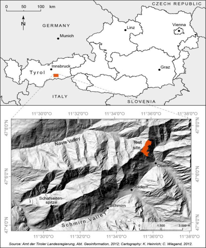
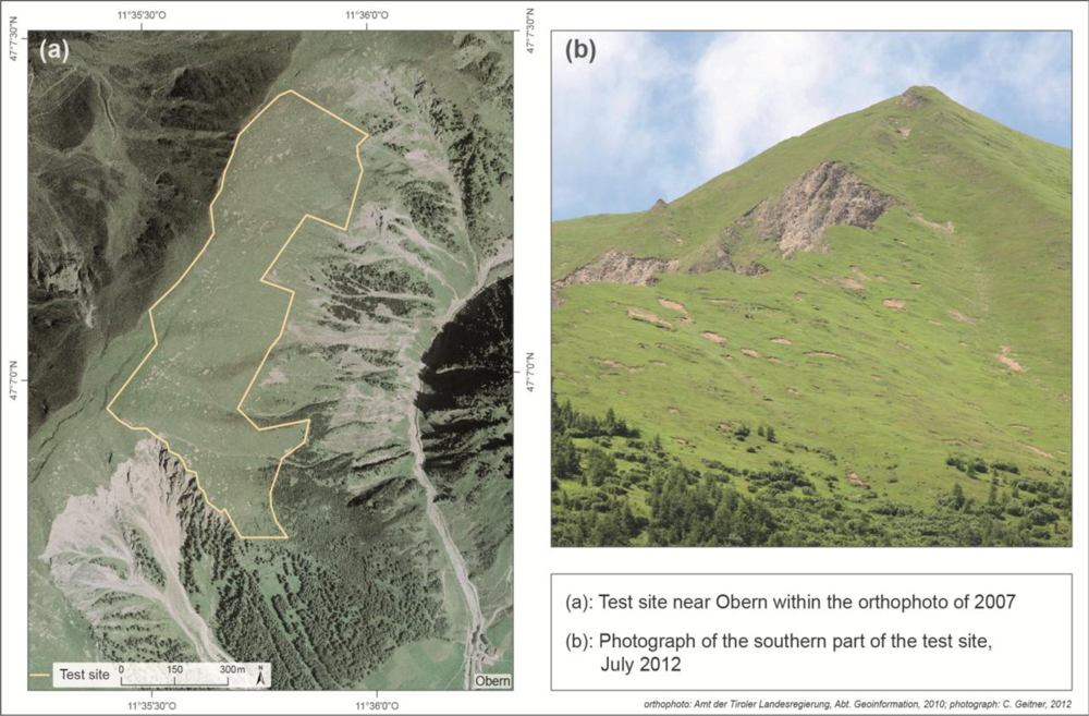
2. Site Description
3. Data Set
4. Segmentation Workflow
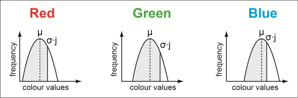
5. Parameter Setting
6. Results
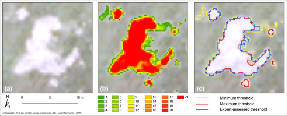
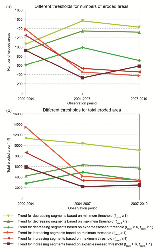
6.1. Comparison of Minimum, Maximum and Expert-Assessed Thresholds for the Segmentation of Eroded Areas
6.2. Occurrence of Erosions in the Four Different Years
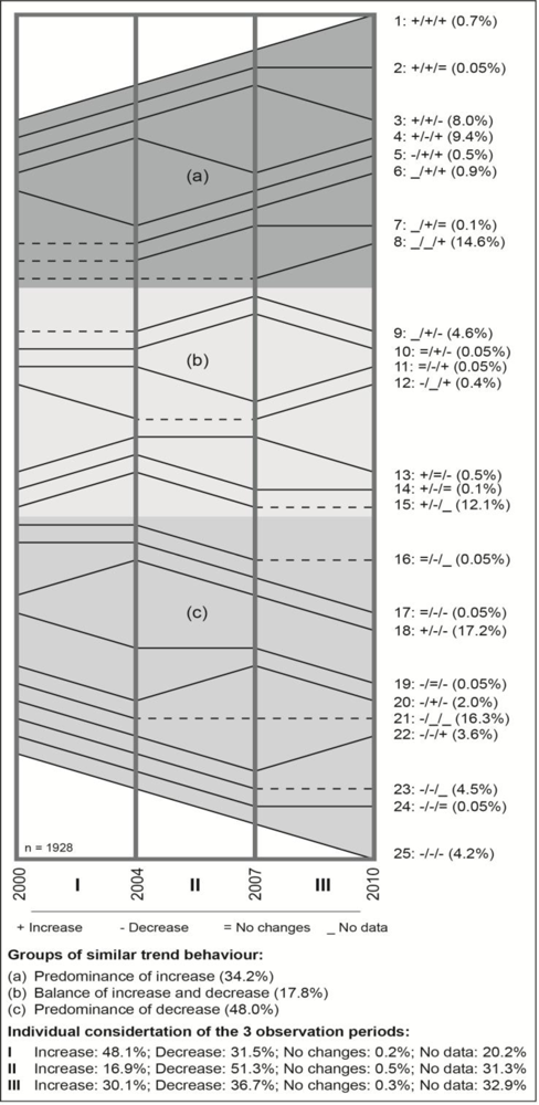
6.3. Qualitative Changes of Classified Eroded Areas between 2000 and 2010
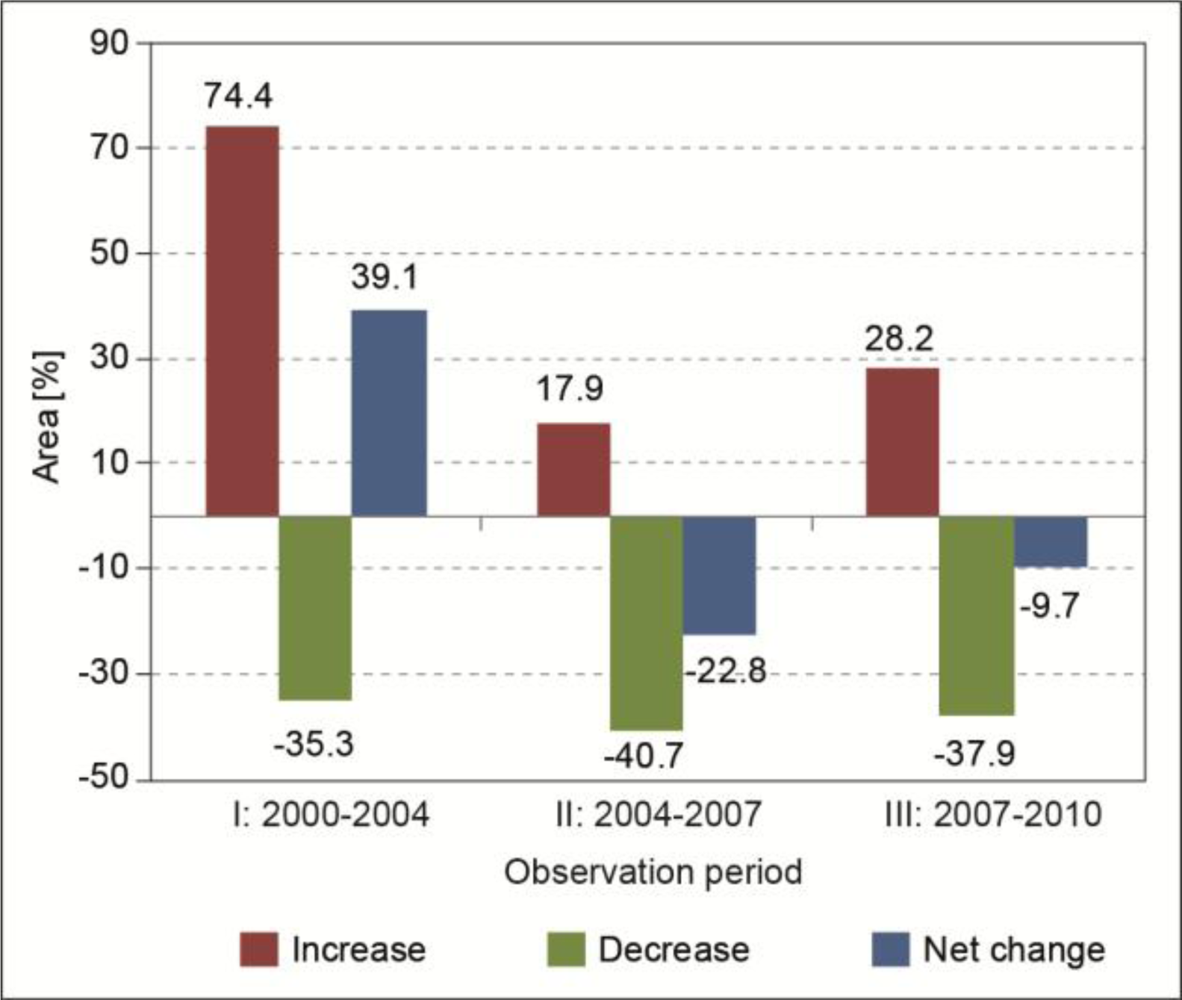
6.4. Quantitative Changes of Classified Eroded Areas between 2000 and 2010
7. Discussion
7.1. Reliability of Imagery
7.2. Reliability of Segmentation
7.3. Changes in Shallow Erosion Size between 2000 and 2010
8. Conclusions and Further Applications
Acknowledgments
- Conflict of InterestThe authors declare no conflict of interest.
References
- MacDonald, D.; Crabtree, J.R.; Wiesinger, G.; Dax, T.; Stamou, N.; Fleury, P.; Gutierrez Lazpita, J.; Gibon, A. Agricultural abandonment in mountain areas of Europe: Environmental consequences and policy response. J. Environ. Manage. 2000, 59, 47–69. [Google Scholar]
- Chemini, C.; Rizzoli, A. Land use change and biodiversity conservation in the Alps. J. Mt. Ecol. 2003, 7 Suppl., 1–7. [Google Scholar]
- Tasser, E.; Leitinger, G.; Pecher, C.; Tappeiner, U. Agricultural Changes in the European Alpine Bow and Their Impact on Other Policies. Proceedings of the 16th Symposium of the European Grassland Federation, Gumpenstein, Austria, 29–31 August 2011; pp. 27–38.
- Glade, T. Landslide occurrence as a response to land use change: A review of evidence from New Zealand. Catena 2003, 51, 297–314. [Google Scholar]
- Tasser, E.; Mader, M.; Tappeiner, U. Effects of land use in alpine grasslands on the probability of landslides. Basic Appl. Ecol. 2003, 4, 271–280. [Google Scholar]
- Meusburger, K.; Alewell, C. Impacts of anthropogenic and environmental factors on the occurrence of shallow landslides in an alpine catchment (Urseren Valley, Switzerland). Nat. Hazards Earth Syst. Sci. 2008, 8, 509–520. [Google Scholar] [Green Version]
- Soldati, M.; Corsini, A.; Pasuto, A. Landslides and climate change in the Italian Dolomites since the Late glacial. Catena 2004, 55, 141–161. [Google Scholar]
- Beniston, M. Mountain weather and climate: A general overview and a focus on climate change in the Alps. Hydrobiologia 2006, 562, 3–16. [Google Scholar]
- Crozier, M.J. Deciphering the effect of climate change on landslide activity: A review. Geomorphology 2010, 124, 260–267. [Google Scholar]
- Chiang, S.-H.; Chang, K.-T. The potential impact of climate change on typhoon-triggered landslides in Taiwan, 2010–2099. Geomorphology 2011, 133, 143–151. [Google Scholar]
- Gobster, P.H.; Nassauer, J.I.; Daniel, T.C.; Fry, G. The shared landscape: What does aesthetics have to do with ecology? Landscape Ecol 2007, 22, 959–972. [Google Scholar]
- Mantovani, F.; Soeters, R.; Van Westen, C.J. Remote sensing techniques for landslide studies and hazard zonation in Europe. Geomorphology 1996, 15, 213–225. [Google Scholar]
- Van Westen, C.J.; Lilie Getahun, F. Analyzing the evolution of the Tessina landslide using aerial photographs and digital elevation models. Geomorphology 2003, 54, 77–89. [Google Scholar]
- Metternicht, G.; Hurni, L.; Gogu, R. Remote sensing of landslides: An analysis of the potential contribution to geo-spatial systems for hazard assessment in mountainous environments. Remote Sens. Environ. 2005, 98, 284–303. [Google Scholar]
- Moine, M.; Puissant, A.; Malet, J.-P. Detection of Landslides from Aerial and Satellite Images with a Semi-Automatic Method. Application to the Barcelonette Basin (Alpes-de-Haute-Provence, France). Proceedings of International Conference Landslide Processes: From Geomorphological Mapping to Dynamic Modelling, CERG, Strasbourg, France, 6–7 February 2009; pp. 63–68.
- Bishop, M.P.; James, L.A.; Shroder, J.F.; Walsh, S.J. Geospatial technologies and digital geomorphological mapping: Concepts, issues and research. Geomorphology 2012, 137, 5–26. [Google Scholar]
- Cardinali, M.; Reichenbach, P.; Guzzetti, F.; Ardizzone, F.; Antonini, G.; Galli, M.; Cacciano, M.; Castekkani, M.; Salvati, P. A geomorphological approach to the estimation of landslide hazards and risks in Umbria, Central Italy. Nat. Hazards Earth Syst. Sci. 2002, 2, 57–72. [Google Scholar]
- Alewell, C.; Meusburger, K.; Brodbeck, M.; Bänninger, D. Methods to describe and predict soil erosion in mountain regions. Landscape Urban Plan. 2008, 88, 46–53. [Google Scholar]
- Van Westen, C.J.; Castellanos, E.; Kuriakose, S.L. Spatial data for landslide susceptibility, hazard, and vulnerability assessment: An overview. Eng. Geol. 2008, 102, 112–131. [Google Scholar]
- Hervás, J.; Barredo, J.; Rosin, P.; Pasuto, A.; Mantovani, F.; Silvano, S. Monitoring landslides from optical remotely sensed imagery: The case history of Tessina landslide, Italy. Geomorphology 2003, 54, 63–75. [Google Scholar]
- Borghuis, A.M.; Chang, K.; Lee, H.Y. Comparison between automated and manual mapping of typhoon-triggered landslides from SPOT-5 imagery. Int. J. Remote Sens. 2007, 28, 1843–1856. [Google Scholar]
- Hay, G.J.; Castilla, G. Geographic Object-Based Image Analysis (GEOBIA): A New Name for A New Discipline. In Object-Based Image Analysis—Spatial Concepts for Knowledge-Driven Remote Sensing Applications; Blaschke, T., Lang, S., Hay, G., Eds.; Springer: Berlin/Heidelberg, Germany, 2008; pp. 75–89. [Google Scholar]
- Martha, T.R.; Kerle, N.; Jetten, V.; van Westen, C.J.; Kumar, K.V. Characterising spectral, spatial and morphometric properties of landslides for semi-automatic detection using object-oriented methods. Geomorphology 2010, 116, 24–36. [Google Scholar]
- Lu, P.; Stumpf, A.; Kerle, N.; Casagli, N. Object-oriented change detection for landslide rapid mapping. IEEE Geosci. Remote Sens. Lett. 2011, 8, 701–705. [Google Scholar]
- Stumpf, A.; Kerle, N. Object-oriented mapping of landslides using Random Forests. Remote Sens. Environ. 2011, 115, 2564–2577. [Google Scholar]
- Hölbling, D.; Füreder, P.; Antolini, F.; Cigna, F.; Casagli, N.; Lang, S. A semi-automated object-based approach for landslide detection validated by persistant scatterer interferometry measures and landslide inventories. Remote Sens. 2012, 4, 1310–1336. [Google Scholar]
- Van den Eeckhaut, M.; Kerle, N.; Poesen, J.; Hervás, J. Object-oriented identification of forested landslides with derivates of single pulse LiDAR data. Geomorphology 2012, 173–174, 30–42. [Google Scholar]
- Schauer, T. Die Blaikenbildung in den Alpen. Schriftenreihe des Bayerischen Landesamtes für Wasserwirtschaft 1975, 1, 1–29. [Google Scholar]
- Van Asch, T.W.J.; Buma, J.; Van Beek, L.P.H. A view on some hydrological triggering systems in landslides. Geomorphology 1999, 30, 25–32. [Google Scholar]
- Lateltin, O.; Haemmig, C.; Raetzo, H.; Bonnard, C. Landslide risk management in Switzerland. Landslides 2005, 2, 313–320. [Google Scholar]
- Laatsch, W.; Grottenthaler, W. Typen der Massenverlagerung in den Alpen und ihre Klassifikation. Forstwissen. Centralbl. 1972, 91, 309–339. [Google Scholar]
- Wiegand, C.; Geitner, C. Flachgründiger Abtrag auf Wiesen- und Weideflächen in den Alpen - Wissensstand, Datenbasis und Forschungsbedarf. Mitt. Österr. Geogr. G. 2010, 152, 130–162. [Google Scholar]
- Dilo, A.; Kraipeerapun, P.; Bakker, W.; de By, R.A. Storing and Handling Vague Spatial Objects. Proceedings of the 15th International Workshop on Database and Expert Systems Applications, DEXA, Zaragoza, Spain, 30 August–3 September 2004; pp. 945–950.
- Fisher, P. Models of Uncertainty in Spatial Data. In Geographical Information Systems: Principles, Techniques, Management and Applications (Volume 1); Longley, P., Goodchild, M.F., Maguire, D.J., Rhind, D.W., Eds.; John Wiley and Sons: New York, NY, USA, 1999; pp. 191–205. [Google Scholar]
- Cohen, A.; Gotts, N. The ‘egg-yolk’ Representation of Regions with Indeterminate Boundaries. In Geographic Objects with Indeterminate Boundaries; Burrough, P.A., Frank, A.U., Eds.; Taylor and Francis: London, UK, 1996; pp. 171–187. [Google Scholar]
- Auer, I.; Hiebl, J.; Reisenhofer, S.; Böhm, R.; Schöner, W. ÖKLIM 1971–2000—Aktualisierung des Digitalen Klimaatlas Österreich 1961–1990; Projektendbericht; ZAMG: Wien, Austria, 2010. [Google Scholar]
- Brandner, R. Geologie und Tektonik. Geologische und Tektonische Übersichtskarte von Tirol. Begleittexte IX; Tirol Atlas: Innsbruck, Austria, 1985; p. 1. [Google Scholar]
- Research Group—Gruppo di Ricerca Consorzio Ferrara Ricerche (CFR), BBT-SE Geological Map 1:25.000 Map Sheets 1 and 2; Universität Innsbruck, Geologische Bundesanstalt (GBA): Innsbruck, Austria, 2006; p. 2.
- TIRIS, Land Tirol, Amt der Tiroler Landesregierung–Tiris. 2010.
- Lillesand, T.M.; Kiefer, R.W.; Chipman, J.W. Remote Sensing and Image Interpretation; Wiley and Sons: New York, NY, USA, 2008. [Google Scholar]
- Frank, A. Why is Scale an Effective Descriptor for Data Quality? The Physical and Ontological Rationale for Imprecision and Level of Detail. In Research Trends in Geographic Information Science; Navratil, G., Ed.; Springer: Berlin/Heidelberg, Germany, 2009; pp. 39–57. [Google Scholar]
- Auerswald, K. Gravitative Bodenverlagerung. In Bodenerosion und Bodenschutz—Analyse und Bilanz eines Umweltproblems; Richter, G., Ed.; Wiss. Buchges.: Darmstadt, Germany, 1998; pp. 61–67. [Google Scholar]
- CIPRA. Alpine Convention Protocol on the Implementation of the Alpine Convention of 1991 in the field of soil conservation. Offic. J. Eur. Union 2005, 48, 29–35.


| 2000 | 2004 | 2007 | 2010 | |
|---|---|---|---|---|
| Number of eroded areas | 1,018 | 1,202 | 919 | 1,013 |
| Total eroded area (m2) | 9,350 | 13,460 | 9,725 | 9,498 |
| Maximum size of e.a.* (m2) | 175 | 185 | 188 | 132 |
© 2013 by the authors; licensee MDPI, Basel, Switzerland This article is an open access article distributed under the terms and conditions of the Creative Commons Attribution license ( http://creativecommons.org/licenses/by/3.0/).
Share and Cite
Wiegand, C.; Rutzinger, M.; Heinrich, K.; Geitner, C. Automated Extraction of Shallow Erosion Areas Based on Multi-Temporal Ortho-Imagery. Remote Sens. 2013, 5, 2292-2307. https://doi.org/10.3390/rs5052292
Wiegand C, Rutzinger M, Heinrich K, Geitner C. Automated Extraction of Shallow Erosion Areas Based on Multi-Temporal Ortho-Imagery. Remote Sensing. 2013; 5(5):2292-2307. https://doi.org/10.3390/rs5052292
Chicago/Turabian StyleWiegand, Christoph, Martin Rutzinger, Kati Heinrich, and Clemens Geitner. 2013. "Automated Extraction of Shallow Erosion Areas Based on Multi-Temporal Ortho-Imagery" Remote Sensing 5, no. 5: 2292-2307. https://doi.org/10.3390/rs5052292