Quantifying Dynamics in Tropical Peat Swamp Forest Biomass with Multi-Temporal LiDAR Datasets

Abstract

Tropical peat swamp forests in Indonesia store huge amounts of carbon and are responsible for enormous carbon emissions every year due to forest degradation and deforestation. These forest areas are in the focus of REDD+ (reducing emissions from deforestation, forest degradation, and the role of conservation, sustainable management of forests and enhancement of forest carbon stocks) projects, which require an accurate monitoring of their carbon stocks or aboveground biomass (AGB). Our study objective was to evaluate multi-temporal LiDAR measurements of a tropical forested peatland area in Central Kalimantan on Borneo. Canopy height and AGB dynamics were quantified with a special focus on unaffected, selective logged and burned forests. More than 11,000 ha were surveyed with airborne LiDAR in 2007 and 2011. In a first step, the comparability of these datasets was examined and canopy height models were created. Novel AGB regression models were developed on the basis of field inventory measurements and LiDAR derived height histograms for 2007 (r² = 0.77, n = 79) and 2011 (r² = 0.81, n = 53), taking the different point densities into account. Changes in peat swamp forests were identified by analyzing multispectral imagery. Unaffected forests accumulated on average 20 t/ha AGB with a canopy height increase of 2.3 m over the four year time period. Selective logged forests experienced an average AGB loss of 55 t/ha within 30 m and 42 t/ha within 50 m of detected logging trails, although the mean canopy height increased by 0.5 m and 1.0 m, respectively. Burned forests lost 92% of the initial biomass. These results demonstrate the great potential of repetitive airborne LiDAR surveys to precisely quantify even small scale AGB and canopy height dynamics in remote tropical forests, thereby featuring the needs of REDD+.

1. Introduction

Considering the global climate change, efforts are being made to reduce global greenhouse gas emissions. One example of such a climate change mitigation mechanism is REDD+ which aims at reducing emissions from deforestation, forest degradation, and the role of conservation, sustainable management of forests and enhancement of forest carbon stocks [1]. In the focus of REDD+ projects are tropical forests which are huge carbon reservoirs comprising 40% of the terrestrial carbon (C) [2,3]. Tropical peatlands accumulate additional carbon in thick belowground peat deposits which are sustained by intact forests on top of it. The largest known tropical peat deposits occur in Southeast Asia, especially in Indonesia where 55–58 Gt·C is stored belowground and 18.6 Gt·C aboveground in forests [4–6]. Deforestation, forest degradation, and peatland degradation in Southeast Asia produce considerable carbon emissions (more than 220 Mt·C·y⁻¹) [7,8]. Between 1997 and 2006, these activities were responsible for 23% of the total anthropogenic CO₂ emissions worldwide [9]. Particularly, Indonesia became one of the largest carbon emitters worldwide, mostly caused by degradation and deforestation of its peatland areas and forests due to large scale agricultural development and exploitation of forest timber resources [10]. Once the forest is degraded, e.g., through logging activities, the fire vulnerability increases [11]. As a result of these activities and consequential emission rates, Indonesia became a prime target for REDD+ projects. REDD+ intends for conditional payments to developing countries reducing emissions. In October 2009, Norway and Indonesia concluded a landmark deal that includes a payment to Indonesia up to one billion USD for forest conservation and slowing down deforestation and greenhouse gas emission rates. Although, Indonesia agreed to halt the license of new logging concessions (on peatlands), large parts of selective logged forests are excluded from this moratorium which means that logged forests are highly vulnerable to re-logging and conversion to plantations [12].

It is important to distinguish between managed or legal, and unplanned or illegal selective logging due to the different impacts on forests. Managed logging constructs extensive infrastructure, for example substantial logging roads, railways along which the logs are being transported, and landing facilities. In contrast, illegal logging operations have no budget and equipment to establish regular roads or railways and their access tracks into the forest are limited. Illegal logging trails follow natural features, such as streams, drainage channels, or abandoned logging tracks, and their spatial pattern is clearly different from the straight extensive infrastructure of legal logging operations [13]. In Central Kalimantan, authorized and illegal logging increased in the 1990s as a direct result of the Mega Rice Project (MRP) which was initiated by the Indonesian government in 1995. The objective was to convert one million hectare of forest for rice cultivation. For this purpose, about 4,000 km of drainage and irrigation channels were excavated into the peatlands, which allowed access into previously inaccessible peat swamp forests. Active illegal logging, which causes vast forest degradation, still takes place in Central Kalimantan’s forests, even if no new logging concessions are granted. The level of degradation is dependent on the forest type and its accessibility. In Borneo, dipterocarp forests provide easy access due to the firm ground and are therefore often affected by logging using bulldozers [14,15]. In contrast, the access for heavy machinery is restricted to peat swamp forests due to the soft ground [16]. Hence, peat swamp forests, which often contain high densities of valuable timber, are logged by human power and the logs are mainly transported on nearby water courses. This way of logging is much less destructive than mechanized logging occurring in dipterocarp forests [17].

Implementation of REDD+ policies depends on accurate and precise estimates of emissions avoided at national scale. In general, forest carbon stocks are derived from aboveground biomass (AGB) by assuming a carbon content of 50% [18]. The most effective monitoring is based on satellite or airborne observations due to the inaccessibility of the forests [19]. As no remote sensing instrument can directly measure AGB, field inventory measurements are mandatory for both calibrating and validating spatial estimations of AGB [18]. The use of LiDAR (light detection and ranging) measurements has rapidly evolved in the last years due to the ability to precisely quantify the vertical structure of the vegetation and forest attributes such as canopy height distribution, tree height, and crown diameter [20–23].

Many studies have demonstrated the great potential of airborne LiDAR to precisely predict AGB in tropical forests [24–26] whereby only few studies have been conducted in the special ecosystem of peat swamp forests [27–31]. Different point cloud statistics of the vegetation height and canopy cover were tested for their performance to predict AGB in peat swamp forests using linear, multiple linear and power functions. Appropriate parameters to estimate AGB were found to be relative height quartiles (r² = 0.71, RMSE = 115.2 t/ha or r² = 0.7, RMSE = 28.6 t/ha) [27,31] and other LiDAR point height distributions such as Quadratic Mean Canopy Height (QMCH) (r² = 0.84) or Centroid Height (CH) (r² = 0.75, RMSE = 20.5 t/ha and r² = 0.88, RMSE = 106 t/ha) [28,29]. Jubanski et al. showed that the AGB regression models can be improved by using the point density as input [29]. Multi-temporal LiDAR measurements offer tremendous potential for REDD+ requirements. It is possible to detect small scale changes in the canopy height or AGB because height and intensity metrics have been proven to be reproducible [32,33]. For example, Dubayah et al. [34] conducted a multi-temporal LiDAR study in Costa Rica and proved that old growth forests have a slower height growth rate (−0.33 m ± 4.09 m) compared to secondary forests (2.08 m ± 3.71 m) and accumulate therefore less biomass per hectare per year (0.3 t·ha⁻¹·y⁻¹ compared to 3.6 t·ha⁻¹·y⁻¹).

The present study analyzed multi-temporal LiDAR and field inventory measurements to investigate forest dynamics and AGB changes in tropical peat swamp forests on Borneo. Airborne LiDAR data were acquired in 2007 and 2011 and the comparability of both datasets was examined. AGB regression models were developed and changes in canopy height and AGB were quantified with a special focus on undisturbed, selective logged and burned peat swamp forests.

2. Materials and Methods

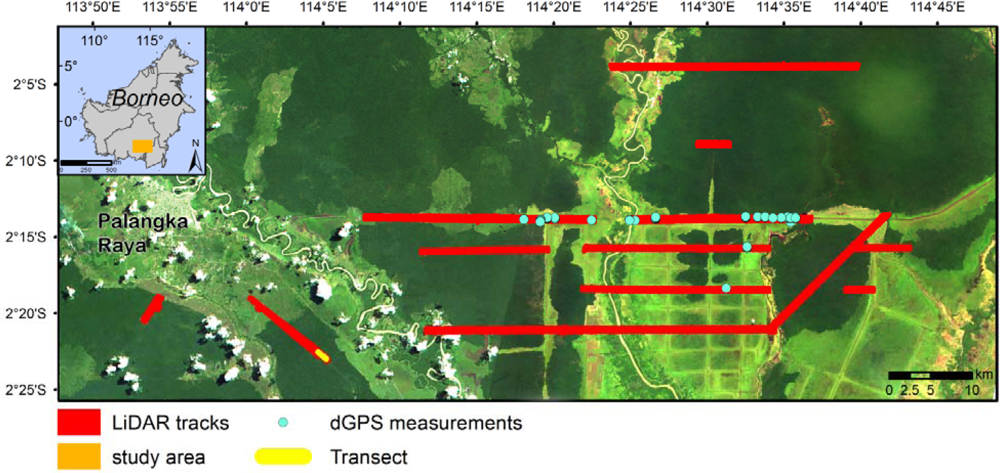
2.1. Study Site

The study area is located east of Palangka Raya, the capital of the province Central Kalimantan, on the island of Borneo, Indonesia (Figure 1). The predominant vegetation type is peat swamp forest which has been under severe anthropogenic pressure for the last three decades, mainly through timber extraction and agricultural conversion [13,35]. The most severe impact was caused by the MRP and the resulting degradation lead to recurrent fires that destroyed approximately 50% of the forest cover in the past two decades [10]. Another driver of forest degradation is illegal selective logging which causes small scale impacts in the forest canopy. Valuable trees are felled, cut into appropriate lengths and then dragged along narrow skid trails to the nearest river or canal where they are transported away. Legal selective logging occurred during the 1980s and 1990s, thereby creating extensive infrastructure. Railways were built to grant access to the highly inaccessible peat swamp forests (Figure 2).

2.2. Data

2.2.1. Field Inventory Data

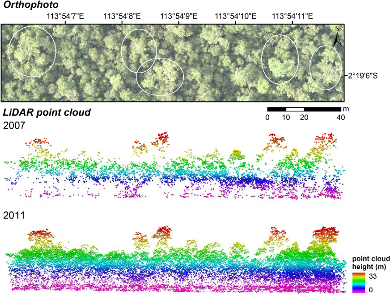
Field inventory campaigns were conducted in the years 2008, 2010, and 2011 whereby inventory plots with different plot sizes were established in forested and regrowing areas. The sample plot design of the field inventory was based on the guidelines provided by Pearson et al. [36]. The plots were distributed over the spatial extent of the LiDAR tacks thereby covering the whole biomass range from woody regrowth to mature forest. Permanent inventory plots were not available due to the inaccessibility of the forests and the ongoing deforestation.

In forested areas, three circular nested plots with radii of 4 m, 14 m, and 20 m were recorded. Inside each nest, trees of a certain DBH (diameter at breast height) were measured depending on degradation intensity: 2 cm to 10 cm or 5 cm to 20 cm (within the 4 m radius), 10 cm to 20 cm or 20 cm to 50 cm (within 14 m radium), and greater than 20 cm or 50 cm (within 20 m radius). In regrowing areas, rectangular plots of 20 m × 50 m were used and all saplings and trees within this area were recorded.

Within both plot types, the following parameters were recorded: DBH, tree height, and tree species in order to estimate their wood density. Tree specific wood densities were derived from databases provided by Chudnoff [37], World Agroforestry Centre [38], and IPCC [39]. If the tree species could not be identified, an average specific wood density for Asian tropical trees of 0.57 Mg·m⁻³, was applied [40].

DBH, tree height, and wood specific density of each tree was used to calculate AGB (t/ha) using a combination of allometric models from Hughes et al. [41] for saplings (if DBH < 5 cm and height ≤ 1.3 m) or trees (if DBH < 5 cm and height > 1.3 m) and Chave et al. [42] for moist tropical forest stands including DBH and tree height (if DBH ≥ 5 cm and height > 1.3 m):

$$\mathit{AGB}=\{\begin{array}{ll}{10}^{-6}\cdot e^{4.7472+1.0915\cdot \text{ln}\left({\mathit{DBH}}^2\right)}\hfill & \mathit{if} \mathit{DBH}<5\mathit{cm} \mathit{and} h\le 1.3m\hfill \\ 1.14\cdot {10}^{-6}\cdot e^{4.9375+1.0583\cdot \text{ln}(\mathit{DBH}?}\hfill & \mathit{if} \mathit{DBH}<5\mathit{cm} \mathit{and} \mathit{h}>1.3m\hfill \\ e^{-2.977+\text{ln}\left(\rho \cdot {\mathit{DBH}}^2\cdot h\right)}\hfill & \mathit{if} \mathit{DBH}\ge 5\mathit{cm} \mathit{and} \mathit{h}>1.3m\hfill \end{array}$$

(1)

where DBH is diameter at breast height, h is tree height, and ρ is wood specific density.

Altogether, 26 plots were sampled in 2008 which were located within the LiDAR tracks of 2007, ranging from 8.7 t/ha to 458.5 t/ha, and 53 plots were sampled in 2010 and 2011 which were inside the LiDAR tracks of 2011 and ranged from 0.0 t/ha to 375 t/ha.

2.2.2. LiDAR Data

LiDAR measurements were collected during the dry seasons (May to October) in 2007 and 2011, respectively, thereby avoiding any influence of standing water during the DTM generation. The 2007 acquisition was conducted in August with a Riegl LMS-Q560 flown 500 m aboveground. Full-waveform LiDAR data was recorded with a half scan angle of ±30°. Each LiDAR transect was generated by a single flight line, thus no strip matching was applied. In 2011, an Optech Orion M200 was used and data were acquired between August and October at a height of 800 m aboveground. Full-waveform LiDAR data were recorded with a half scan angle of ±11°. A strip adjustment procedure was applied resulting in an average vertical accuracy of a root mean square error (RMSE) of 0.036 m. Further data specifications and acquisition details are provided in

Table 1. Specifications of LiDAR acquisitions.

Specification	2007	2011
LiDAR system	Riegl LMS-Q560	Optech Orion M200
Acquisition date	5–10 August	15 August–14 October
Power	100 KHz	100 KHz
Nominal Altitude	500 m	800 m
Wavelength	1.5 μm	1.064 μm
Half Scan angle	±30°	±11°
Average point density	1.5 points/m2	10.7 points/m2

. The specifications of both LiDAR instruments differed in some aspects, e.g., scan angle, flight height, and wavelength, but the most important difference was in terms of point density. Figure 3 illustrates the difference in LiDAR survey point density between 2007 (1.5 points/m²) and 2011 (10.7 points/m²) within an undisturbed peat swamp forest. In order to minimize problems due to the scan angle difference, 10% of the swath width (25 m of each side of the strip) of the 2007 LiDAR tracks was excluded as a reduction in point density of 25% to 40% from nadir to the edge of the swath was observed. Therefore weighing the plots accordingly to their point densities will indirectly take into account the scan geometry. In addition, 80% of the 2008 field plots were collected within a swath of ±15°.

During the 2011 LiDAR acquisition, photos were taken from the aircraft and were processed to orthophotos with a spatial resolution of 0.25 m. The two LiDAR campaigns resulted in a total overlapping area of 11,726 ha and the land cover comprised peat swamp forests, partly affected by former and recent selective logging, old burn scars, fern, grassland, bushes, and agricultural land.

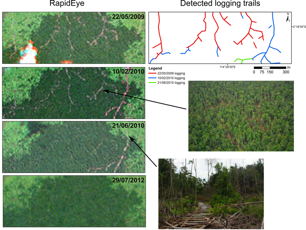
2.2.3. Multispectral Imagery

High-resolution RapidEye imagery has been proven to detect small scale logging in peat swamp forests and was therefore chosen to monitor logging activities and fire impacts between both LiDAR acquisitions [43]. The RapidEye satellite system is a constellation of five identical satellites, which were launched in August 2008, and the images have a pixel resolution of 5 m. Scenes used in this study were acquired on 22 May 2009, 28 July 2009, 10 February 2010, 11 February 2010, 21 June 2010, 18 August 2011, and 29 July 2012, and were atmospherically corrected and co-registered.

Medium resolution Landsat imagery was used to analyze historical managed logging during the 1980s and early 1990s. Landsat satellites have acquired scenes since 1972, mostly with a spatial resolution of 30 m. Former managed logging was investigated on the basis of a Landsat scene from 30 June 1991, which was atmospherically corrected and co-registered (Figure 2). All logging activities before that date were included in the analyses.

2.3. Data Analysis

In a first step, the LiDAR point clouds of 2007 and 2011 were compared to each other and the effect of different point densities was examined. As set out in Table 1, the mean point density differed by a factor of 7. Figure 3 shows an orthophoto taken in 2011 and the corresponding LiDAR point clouds of 2007 and 2011 within an unaffected peat swamp forest. Tree crowns of emergent trees are easily identifiable and are indicated by circles in the orthophoto. Although the point density differences are clearly visible, the relative distribution over the different vegetation layers is similar. In the 2007 data, the relative number of LiDAR returns from the ground and lower vegetation layer is less than in the 2011 data. Therefore, height histograms and consequently height histograms of both LiDAR measurements are slightly different. For this reason, it was reasonable to develop separate AGB regression models for 2007 and 2011.

2.3.1. LiDAR Filtering and DTM Generation

A crucial step within the digital terrain model (DTM) generation is the LiDAR filtering. A hierarchic robust filter was applied to the LiDAR point clouds, separating the ground and non-ground (vegetation) points [44]. The linear adaptable prediction interpolation (kriging) was utilized to generate DTMs with a resolution of 1 m. The accuracy of the DTMs was evaluated on the basis of field derived differential Global Positioning System (dGPS) measurements. Altogether, 93 dGPS measurements were available within both LiDAR tracks covering different land cover classes (peat swamp forest, open forest, burn scars, ferns, and shrubs) (Figure 1). The 2007 and 2011 DTM resulted in RMSE = 0.41 m and RMSE = 0.16 m, respectively. In comparison to each other, the DTM featured RMSE = 0.37 m (Figure 4). The DTMs were further utilized for the CHM creation and AGB estimation. Due to the difference of both datasets, separated CHMs and AGB models for 2007 and 2011, were generated. Therefore, the acquisition difference does not influence the analyses as relative heights were used and are supposed to be stable [45,46].

2.3.2. Canopy Height Models

CHMs of both years with a resolution of 1 m were produced by calculating the difference between the elevation of the digital surface model (DSM) and the underlying terrain of the DTM. For the DSM the highest point was chosen within a grid of 1 m. Pixels containing no data were filled using the highest point of the neighborhood and the morphological operator “closing” [47]. The changes of the CHMs between 2007 and 2011 were analyzed by calculating the difference of both models and subsequent median filtering. The relative accuracy between both CHMs is similar to the accuracy of the DTMs (RMSE = 0.37 m).

2.3.3. Biomass Estimation

Due to the differences of both LiDAR measurements, especially in point density, each acquisition was treated as an independent assessment and the biomass models were therefore developed separately. Similarly, Hudak et al. [45] used LiDAR measurements with significant differences in point densities and found out that different point densities do not affect AGB estimations if LiDAR measurements were independently analyzed.

Only 26 field inventory plots were available for the 2007 LiDAR analysis and there were not sufficient data to develop an accurate regression model. Hence, the 2011 LiDAR point density of the 2011 field inventory plots was reduced, resulting in a similar point density as the 2007 data, and added to the 2007 analysis as reference data in order to enlarge the AGB reference dataset for a significant analysis. The LiDAR point density of 2011 was reduced by taking the highest and lowest point within a square with a side length of 1 m. The 2011 plots within the reduced LiDAR data of 2011 resulted in a mean point density of 1.99 points/m² whereas the 2007 plots within the 2007 LiDAR data had an average point density of 1.52 points/m². In 2011, sufficient field inventory plots (n = 53) were available to develop an accurate AGB regression model.

Previous studies revealed that the centroid height is an appropriate height parameter of the LiDAR point cloud to estimate AGB in tropical forests taking also the point distribution over the different vegetation layers into account [27–29]. It was therefore used in this study to estimate AGB and its changes. LiDAR height histograms were calculated by normalizing all points within a grid of 35 m (similar to the size of the largest field inventory plot) to the ground using the DTMs as reference. A height interval of 0.5 m was defined and the number of points within this interval was stored in form of a histogram. The first height interval was considered as ground return and therefore excluded from the further processing. The centroid height (CH) of the height histogram was calculated by weighing each 0.5 m height interval with the relative number of LiDAR points stored within this interval. CH was related to field inventory derived AGB and regression models were developed. Jubanski et al. [29] showed that the accuracy of AGB estimations derived from LiDAR height histograms increased with higher point densities. For this reason, point density was also implemented in the regression in form of a weighting factor.

The commonly used power functions [25,26,29] resulted in significant overestimations in the higher biomass range of our study area. For this reason, we developed a novel, more appropriate AGB regression model, which is a combination of a power function (in the lower biomass range up to a certain threshold CH₀) and a linear function (in the higher biomass range). The threshold of CH₀ was determined by increasing the value of CH₀ in steps of 0.001 m by identifying the lowest RMSE. The linear function is the tangent through CH₀ and was calculated on the basis of the first derivative of the power function:

$$\mathit{AGB}=\{\begin{array}{ll}a\cdot {\mathit{CH}}^b\hfill & \mathit{if} \mathit{CH}\le {\mathit{CH}}_0\hfill \\ \left(a\cdot b\cdot {\mathit{CH}}_0^{(b-1)}\right)\left(\mathit{CH}-{\mathit{CH}}_0\right)+a\cdot {\mathit{CH}}_0^b\hfill & \mathit{if} \mathit{CH}>{\mathit{CH}}_0\hfill \end{array}$$

(2)

where CH is the centroid height, CH₀ is the threshold of function change and a, b are coefficients.

The developed AGB regression models were independently validated by the Predictive Power of the Regression (PPR) as carried out by Asner et al. [24]. The PPR is the RMSE determined by running 1,000 iterations of the regression by randomly leaving out 10% of the reference field inventory plots.

The biomass models were applied to all available LiDAR tracks. Changes in biomass were calculated over the four year time period by subtracting the 2007 AGB map from the one of 2011. Positive values thus indicate net biomass gain while negative values indicate loss.

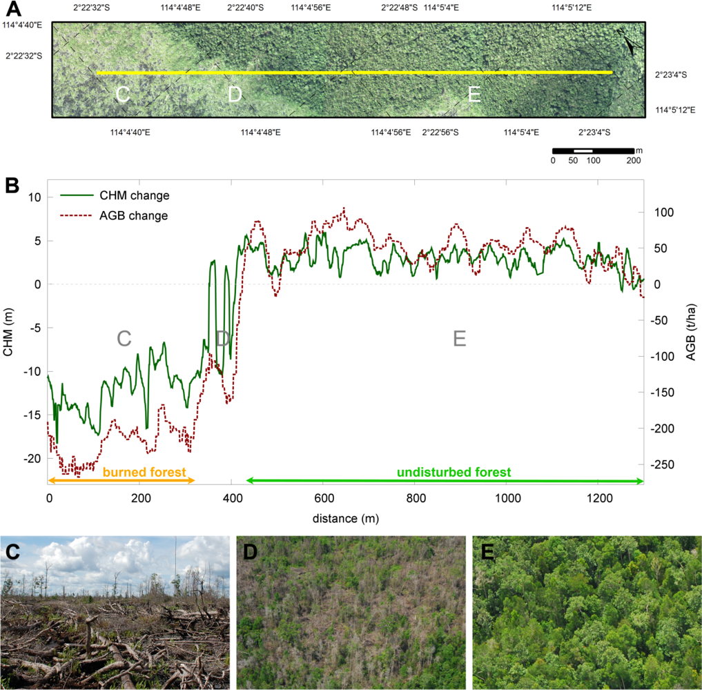
2.3.4. Change Analysis

Changes in canopy height and AGB between 2007 and 2011 were analyzed over the whole study area. The vegetation within the study area is under strong anthropogenic pressure and thus experiences many changes. Multispectral imagery was used to identify unaffected, selective logged and burned peat swamp forests, and changes in canopy height and AGB were quantified within these areas. Logging trails could be easily identified due to the high spatial and temporal resolution of the RapidEye data. On the basis of field surveys, orthophotos and long term experience within the study area as well as lack of literature reference data, an area with a buffer of 30 m and 50 m, respectively, was chosen for the investigation of AGB loss caused by selective logging. It is assumed that loggers do not remove trees that are further away from the logging trail than 50 m because new trails would then be constructed. Additionally, areas affected by former managed selective logging with extensive infrastructure were identified on the basis of a Landsat scene from 30 June 1991. All logging activities before that date were included in the analyses.

3. Results

3.1. Canopy Height Models

Changes in canopy height were evaluated on the basis of CHMs. In unaffected forests, it was possible to identify crowns of emergent trees and to quantify the growth rates. Figure 5(A) depicts the 2007 and 2011 CHM of such a tree crown. Tree height increased by 0.6 m within the four years, from 29.3 m to 29.9 m. An example of a degraded forest area is shown in Figure 5(B). The degradation was most likely caused by felling the trees. The two examples demonstrate that changes in the CHM helped to identify areas of growth and disturbance.

3.2. AGB Regression Models

Due to different point densities of both LiDAR acquisitions, two separated AGB regression models were developed on the basis of a combined power and linear function (Equation (2), Figure 6(A) shows scatterplots of AGB and CH for 2007 and 2011 with the corresponding regressions. The part of the power function in the lower biomass range is depicted in blue and the linear part of the function in the higher biomass range in orange. The size of the reference field inventory plots depends on LiDAR point density, the higher the density, the bigger the dot. Figure 6(B) displays the dependence of CH₀, the threshold of function change, and RMSE for the 2007 and 2011 AGB regression models. The lower the value of CH₀, the lower is the proportion of the power function and the higher the value of CH₀, the lower is the proportion of the linear function. The value with the lowest RMSE is marked and was chosen as CH₀. Figure 6(C) depicts LiDAR derived AGB estimations versus field inventory AGB values of the AGB reference dataset. The 2007 AGB regression model was developed on the basis of 79 field inventory measurements resulting in a coefficient of determination r² = 0.77 with PPR = 54.2 t/ha and CH₀ = 8.086 m. For the 2011 AGB regression model, 53 field inventory plots were available for calibration and validation and resulted in r² = 0.81, PPR = 47.4 t/ha and CH₀ = 8.841 m.

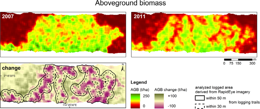
3.3. Change Analyses

The study area comprises several different land covers, such as peat swamp forest, former burned and regrowing areas containing fern, grassland, bushes, and agricultural areas. Due to the high variability, three main categories of change of initial peat swamp forests between both LiDAR acquisitions were evaluated on the basis of multispectral imagery.

First, undisturbed forest areas of 3,393 ha, that had no or no visible impact, were identified. Second, logging trails were identified on the basis of high temporal and spatial resolution RapidEye data. Figure 7 depicts four different RapidEye scenes showing the example of a selective logged area. The narrow skid trail infrastructure, which is clearly visible, was fast evolving and the rapid regrowth of the vegetation after the logging activities stopped hindered the detection of the full extent of logging in the RapidEye images. All skid trails that could be detected with available RapidEye imagery are also shown in Figure 7 (“detected logging trails”). On the basis of repetitive field observations, the area within 30 m and 50 m of the detected logging trails was analyzed and amounted to 67 ha and 113 ha, respectively. Third, forested areas that burned once between both LiDAR acquisitions were evaluated. This is important because recurrent fires further reduce AGB. Altogether, 555 ha of initial peat swamp forests within the study area burned.

Table 2. Quantification of changes in canopy height and AGB of unaffected, selective logged (within 30 m and 50 m of logging trails) or burned peat swamp forests. The mean values and standard deviations (std) are depicted.

Forest Condition	Unaffected		Selective Logged within				Burned
			30 m		50 m
	Mean	std	Mean	std	Mean	std	Mean	std
area (ha)	3,393		67		113		555
CHM 2007 (m)	14.0	5.8	13.5	6.0	13.2	6.0	11.1	6.7
CHM 2011 (m)	16.3	4.7	13.9	5.9	14.2	5.8	1.7	4.0
CHM change (m)	+2.3	1.9	+0.5	3.1	+1.0	3.0	−9.4	5.3
AGB 2007 (t/ha)	203	58	215	62	209	63	154	80
AGB 2011 (t/ha)	223	47	160	57	167	57	12	21
AGB change (t/ha)	+20	33	−55	41	−42	44	−142	77

depicts canopy height and AGB dynamics and the standard deviations (std) indicating the AGB variability within these areas. In undisturbed peat swamp forests, the canopy height increased on average by 2.3 m and accumulated 20 t/ha over this four year time period. In selective logged forests, the canopy height increased on average 0.5 m and mean AGB decreased by 55 t/ha within 30 m of the logging trails whereby a canopy height increase of 1.0 m and AGB loss of 42 t/ha was detected within 50 m of the logging trails. As expected, burned forests experienced an extensive loss in canopy height (9.4 m on average) and AGB (approximately 92%). The initial AGB of burned forests (154 t/ha) was on average lower than of undisturbed peat swamp forest (203 t/ha) which indicates that degraded forests are more vulnerable to fire.

Figure 8 shows AGB of 2007 and 2011 as well as its changes in the selective logged peat swamp forest area of Figure 7. The areas within 30 m and 50 m of the detected logging trails were analyzed and are also depicted. The forest area has already been degraded in 2007, but has further been exploited between both acquisitions which is not only evident from multispectral imagery (Figure 7) but also from AGB loss (Figure 8). The spatial pattern of AGB loss clearly follows the skid trails whereas AGB accumulated in remaining small forest patches.

Figure 9 depicts a transect through a burned and adjacent unaffected peat swamp forest with the changes in canopy height and AGB. The extensive loss of AGB and canopy height is clearly visible within the burned area (C) as well as growth of canopy height and accumulation of AGB in the unaffected area (E). The transition area (D) between the burned and unaffected area is characterized by single remaining trees which increased in height over the four years. This effect is visible in the canopy height change diagram. Even if single remaining trees increased in height, AGB of this transition area was reduced due to the fire impact.

Historical managed logged areas during the 1980s and early 1990s were identified on the basis of a Landsat scene from 30 June 1991. In total, 4,529 ha of the study area (39%) were affected by former managed logging of which 2946 ha were degraded to shrubs, bushes, and grassland in 2007, whereby 110 ha were part of a large scale oil palm plantation. The remaining historical logged area (1,584 ha) was still forested in 2007 of which 1,211 ha remained unaffected between 2007 and 2011. The average biomass of these forests was 219 t/ha in 2007 and 238 t/ha in 2011 with a mean canopy height of 14.2 m and 16.8 m, respectively. In contrast, unlogged and undisturbed forests contained 194 t/ha with a mean canopy height of 13.9 m in 2007 and 214 t/ha with a mean canopy height of 16.0 m in 2011. These results demonstrate that historical logged forests have in general a higher forest biomass than unaffected forests, even though they were degraded 20 years ago. This comparison also revealed that historical logged forests experienced a higher growth rate (on average 2.6 m) during this four year time period than primary forests (on average 2.1 m), thereby accumulating a similar amount of AGB (19 t/ha and 20 t/ha, respectively).

4. Discussion

Implementation of REDD+ projects require accurate carbon or AGB estimations as well as their changes at national level. This study shows that repeat LiDAR measurements are capable of estimating changes in AGB even if data specifications and acquisition details differs from each other. The datasets were comparable when treated as independent assessments by developing two separated AGB regression models. Hudak et al. [45] also compared repetitive LiDAR measurements that had a 30-fold difference in point density and concluded that it does not affect biomass estimations and dynamics when treated as independent assessments with two independently developed regression models. Large scale LiDAR surveys, e.g., at national level, and especially repetitive acquisitions are very expensive and may exceed the financial framework of these projects. A cost-effective possibility would be to upscale accurate regional airborne LiDAR derived carbon estimations and changes with satellite imagery.

The most appropriate regression model to predict AGB from LiDAR derived CH was a combined power and linear function. Although many studies obtained good results for estimating AGB from LiDAR height metrics on the basis of a power function [48–50], we detected significant overestimations in the higher biomass range when using solely a power function. Additionally, AGB estimations derived from the power function were not as accurate as estimations derived from the combined power and linear function. The AGB regression model of 2007 solely based on the power function resulted in r² = 0.75 and PPR = 65.1 t/ha whereas the regression model based on a combined power and linear function resulted in r² = 0.77 and PPR = 54.2 t/ha. Similarly, the AGB model of 2011 based on the power function resulted in r² = 0.78 and PPR = 52.3 t/ha and the combined power and linear function resulted in r² = 0.81 and PPR = 47.4 t/ha. Similarly, Mascaro et al. [51] developed a carbon estimation regression model on the basis of airborne LiDAR canopy height metrics in a tropical forest in Panama and also modified the power function of the AGB regression.

In unaffected peat swamp forests, the mean canopy height increased on average 2.3 m and accumulated 5 t·ha⁻¹·y⁻¹. These unaffected forest areas included primary and secondary forests of different degradation levels as well as different peat swamp forest types. The growth and accumulation rates are an average of fast growth rates, e.g., in previously logged forests and slow growth rates and in primary forests. Sweda et al. [30] and Boehm et al. [52] analyzed some of the same 2007 LiDAR data in combination with another LiDAR dataset also acquired in 2011 within the study area. They found a canopy growth of 1.9 m and an AGB accumulation of 3.7 t·ha⁻¹·y⁻¹. The results might differ from each other mainly due to the spatial extent of the study area.

Canopy height and AGB changes in illegal selective logged areas were quantified within 30 m and 50 m of detected logging trails. As no reference data could be found in literature, the extent of the analyzed area was based on repetitive field observations on ground and during flight surveys as well as long term experience within the study area. It is assumed that trees which are more than 50 m away from the trails are unlikely to be logged because new logging trails would then be constructed in order to overcome the access difficulties in peat swamp forests. Within the 30 m area of the trails, canopy height increased by 0.5 m and AGB was reduced by 55 t/ha which makes up 26% of initial biomass. The analysis of the 50 m area resulted in a canopy height increase of 1.0 m and AGB loss of 42 t/ha which is 20% of initial biomass. Although AGB was reduced in both cases, canopy height increased as a result of fast regrowth. Trees grow fast in height with thin trunks and thus slowly accumulate AGB. No other study on AGB loss due to selective logging in tropical peat swamp forests could be found. Mazzei et al. [53] estimated AGB loss due to small impact logging in the eastern Amazon on the basis of field inventory data to 94.5 t/ha which is equivalent to 23% of the initial AGB. Other studies on managed selective logging also based on field measurements in dipterocarp forests reported an AGB loss between 33% and 56% of the initial forest biomass [14,15]. This comparison emphasizes the different degradation levels caused by selective logging in dipterocarp and peat swamp forests.

The quantitative assessment of burned peat swamp forests revealed that 92% of initial 154 t/ha was lost. Three field inventory measurements were available within the study area before (2008) and after (2010) the fire in 2009. On average, 98% of 187 t/ha was lost due to fire. Hashimotio et al. [54] and Hiratsuka et al. [55] conducted field inventory measurements in East Kalimantan on a burned forest area and found remaining AGB of 8–10 t/ha and 9–17 t/ha, respectively. This comparison shows that the amount of remaining biomass after fire events is similar.

In total, 4,529 ha of the study area were affected by managed selective logging in the 1980s and early 1990s of which 65% were degraded to shrubs, bushes and grassland in 2007 demonstrating the high vulnerability of degraded peat swamp forests. Different growth but similar AGB accumulation rates were detected in former logged (2.3 m and 19 t/ha) and completely unaffected forests (1.9 m and 20 t/ha) demonstrating faster growth rates of secondary forests. Unaffected and unlogged forests contained on average less biomass per hectare than former managed logged forests after 20 years of regrowth. This fact can be explained by different forest types with various species composition. For example, low pole peat swamp forests grow to a maximum height of 20 m. They contain very few commercial tree species and only few of these provide good quality timber [56]. In contrast, tall interior and mixed peat swamp forests reach a maximum height of 45 m and 35 m, respectively, and comprise several tree species of commercial importance. Hence, these forest types are subjected to the most intense logging [56].

With regard to REDD+ projects, it is important to take a closer look at the accuracy of AGB estimations. First, errors associated with field inventory work such as measurements errors or GPS accuracy may influence the AGB reference data. Another potential source of error is the time difference between field inventories and LiDAR acquisitions. These errors are hard to quantify in our analysis. The accuracy of both DTMs to each other resulted in RMSE = 0.37 m within forest, burn scars, fern and shrubs. On a stable surface, the runway of Palangka Raya, the accuracy was much higher (RMSE = 0.07 m). It can therefore be reasonably assumed that the relative accuracy between both CHMs is similar to the DTM accuracy. Therefore, changes in canopy height are within an accuracy of ±0.37 m. Furthermore, the difference of the DTMs is not supposed to have an influence on AGB estimations as height intervals of 0.5 m were chosen. The errors of AGB regression models also influence AGB change calculations. An empirical evidence for the usefulness of AGB quantifications can be found in Table 2. The AGB variability, indicated by the standard deviation, in unaffected forests in 2007 and 2011 is of a similar amount (58 t/ha and 47 t/ha). The AGB gain (5 t·ha⁻¹·y⁻¹) is reasonable compared to other studies [30].

5. Conclusion

This study demonstrates the enormous potential of multi-temporal airborne LiDAR surveys to accurately estimate AGB (aboveground biomass biomass) dynamics in carbon rich tropical peat swamp forests. Due to differences in LiDAR acquisitions, two independent regression models were developed in order to estimate AGB on the basis of the centroid height (CH) of the LiDAR point cloud taking also the point density into account. A novel regression model was developed combining a power and linear function which resulted in more accurate AGB estimates than the common used power function. Changes in canopy height and AGB could be successfully quantified in unaffected, former and recently selective logged, and burned forests revealing the impacts of different degradation levels on tropical peat swamp forests. A more detailed analysis of different and repetitive degradation levels would be helpful to assess the growth and AGB accumulation rates in more detail. A next step could be the investigation of the variability of peat swamp forests considering different forest types and degradation levels leading to a better understanding of the forests and their environment.

References

1. Campbell, B.M. Beyond Copenhagen: REDD plus, agriculture, adaptation strategies and poverty. Glob. Environ. Chang. 2009, 19, 397–399. [Google Scholar]
2. Food and Agriculture Organization (FAO). State of the World’s Forests 2009; Food and Agriculture Organization of the United Nations: Rome, Italy, 2009; Available online: http://www.fao.org/docrep/011/i0350e/i0350e00.htm (accessed on 4 February 2013).
3. Page, S.E.; Hoscilo, A.; Langner, A.; Tansey, K.; Siegert, F.; Limin, S.; Rieley, J.O. Tropical Peatland Fires in Southeast Asia. In Tropical Fire Ecology: Climate Change, Land Use, and Ecosystems Dynamics; Cochrane, M.A., Ed.; Springer-Praxis: Berlin, Germany, 2009; Chapter 9; pp. 263–287. [Google Scholar]
4. Page, S.E.; Rieley, J.O.; Banks, C.J. Global and regional importance of the tropical peatland carbon pool. Glob. Change Biol. 2011, 17, 798–818. [Google Scholar]
5. Jaenicke, J.; Rieley, J.O.; Mott, C.; Kimman, P.; Siegert, F. Determination of the amount of carbon stored in Indonesian peatlands. Geoderma 2008, 147, 151–158. [Google Scholar]
6. Baccini, A.; Goetz, S.; Walker, W.; Laporte, N.; Sun, M.; Sulla-Menashe, D.; Hackler, J.; Beck, P.; Dubayah, R.; Friedl, M.; et al. Estimated carbon dioxide emissions from tropical deforestation improved by carbon-density maps. Nat. Clim. Change 2012, 2, 182–185. [Google Scholar]
7. Couwenberg, J.; Dommain, R.; Joosten, H. Greenhouse gas fluxes from tropical peatlands in south-east Asia. Glob. Change Biol. 2010, 16, 1715–1732. [Google Scholar]
8. Murdiyarso, D.; Hergoualc’h, K.; Verchot, L.V. Opportunities for reducing greenhouse gas emissions in tropical peatlands. Proc. Natl. Acad. Sci. USA 2010, 107, 19655–19660. [Google Scholar]
9. Van der Werf, G.R.; Morton, D.C.; DeFries, R.S.; Olivier, J.G.J.; Kasibhatla, P.S.; Jackson, R.B.; Collatz, G.J.; Randerson, J.T. CO2 emissions from forest loss. Nat. Geosci. 2009, 2, 829. [Google Scholar]
10. Miettinen, J.; Liew, S.C. Two decades of destruction in Southeast Asia’s peat swamp forests. Front. Ecol. Environ. 2012, 10, 124–128. [Google Scholar]
11. Siegert, F.; Ruecker, G.; Hinrichs, A.; Hoffmann, A.A. Increased damage from fires in logged forests during droughts caused by El Nino. Nature 2001, 414, 437–440. [Google Scholar]
12. Edwards, D.P.; Koh, L.P.; Laurance, W.F. Indonesia’s REDD+ pact: Saving imperilled forests or business as usual? Biol. Conserv. 2012, 151, 41–44. [Google Scholar]
13. Boehm, H.D.V.; Siegert, F. The impact of logging and land use change in Central Kalimantan, Indonesia. Int. Peat J. 2004, 12, 3–10. [Google Scholar]
14. Pinard, M.A.; Putz, F.E. Retaining forest biomass by reducing logging damage. Biotropica 1996, 28, 278–295. [Google Scholar]
15. Berry, N.J.; Phillips, O.L.; Lewis, S.L.; Hill, J.K.; Edwards, D.P.; Tawatao, N.B.; Ahmad, N.; Magintan, D.; Khen, C.V.; Maryati, M.; et al. The high value of logged tropical forests: Lessons from northern Borneo. Biodivers. Conserv. 2010, 19, 985–997. [Google Scholar]
16. Whitmore, T.C. Tropical Rain Forests of the Far East; Clarendon Press: Oxford, UK, 1984. [Google Scholar]
17. Felton, A.M.; Engstrom, L.M.; Felton, A.; Knott, C.D. Orangutan population density, forest structure and fruit availability in hand-logged and unlogged peat swamp forests in West Kalimantan, Indonesia. Biol. Conserv. 2003, 114, 91–101. [Google Scholar]
18. Goetz, S.; Dubayah, R. Advances in remote sensing technology and implications for measuring and monitoring forest carbon stocks and change. Carbon Manag. 2011, 2, 231–244. [Google Scholar]
19. Gibbs, H.K.; Brown, S.; Niles, J.O.; Foley, J.A. Monitoring and estimating tropical forest carbon stocks: Making REDD a reality. Envrion. Res. Lett. 2007, 2, 1–13. [Google Scholar]
20. Jung, J.; Crawford, M.M. Extraction of features from LIDAR waveform data for characterizing forest structure. IEEE Geosci. Remote Sens. Lett. 2012, 9, 492–496. [Google Scholar]
21. Vincent, G.; Sabatier, D.; Blanc, L.; Chave, J.; Weissenbacher, E.; Pélissier, R.; Fonty, E.; Molino, J.F.; Couteron, P. Accuracy of small footprint airborne LiDAR in its predictions of tropical moist forest stand structure. Remote Sens. Environ. 2012, 125, 23–33. [Google Scholar]
22. Duncanson, L.; Niemann, K.; Wulder, M. Estimating forest canopy height and terrain relief from GLAS waveform metrics. Remote Sens. Environ. 2010, 114, 138–154. [Google Scholar]
23. Gleason, C.J.; Im, J. A review of remote sensing of forest biomass and biofuel: Options for small-area applications. GISci. Remote Sens. 2011, 48, 141–170. [Google Scholar]
24. Asner, G.P.; Powell, G.V.N.; Mascaro, J.; Knapp, D.E.; Clark, J.K.; Jacobson, J.; Kennedy-Bowdoin, T.; Balaji, A.; Paez-Acosta, G.; Victoria, E.; et al. High-resolution forest carbon stocks and emissions in the Amazon. Proc. Natl. Acad. Sci. USA 2010, 107, 16738–16742. [Google Scholar]
25. Asner, G.P.; Mascaro, J.; Muller-Landau, H.C.; Vieilledent, G.; Vaudry, R.; Rasamoelina, M.; Hall, J.S.; van Breugel, M. A universal airborne LiDAR approach for tropical forest carbon mapping. Oecologia 2012, 168, 1147–1160. [Google Scholar]
26. Mascaro, J.; Detto, M.; Asner, G.P.; Muller-Landau, H.C. Evaluating uncertainty in mapping forest carbon with airborne LiDAR. Remote Sens. Environ. 2011, 115, 3770–3774. [Google Scholar]
27. Kronseder, K.; Ballhorn, U.; Böhm, V.; Siegert, F. Aboveground biomass estimation across forest types at different degradation levels in Central Kalimantan using LiDAR data. Int. J. Appl. Earth Obs. 2012, 18, 37–48. [Google Scholar]
28. Ballhorn, U.; Jubanski, J.; Siegert, F. ICESat/GLAS Data as a measurement tool for peatland topography and peat swamp forest biomass in Kalimantan, Indonesia. Remote Sens. 2011, 3, 1957–1982. [Google Scholar]
29. Jubanski, J.; Ballhorn, U.; Kronseder, K.; Franke, J.; Siegert, F. Detection of large above ground biomass variability in lowland forest ecosystems by airborne LiDAR. Biogeosci. Discuss. 2012, 9, 11815–11842. [Google Scholar]
30. Sweda, T.; Tsuzuki, H.; Maeda, Y.; Boehm, V.; Limin, S.H. Above- and Below-Ground Carbon Budget of Degraded Tropical Peatland Revealed by Multi-temporal Airborne Laser Altimetry. Proceedings of the 14th International Peat Congress, Stockholm, Sweden, 3–8 June 2012.
31. Meyer, V.; Saatchi, S.S.; Chave, J.; Dalling, J.; Bohlman, S.; Fricker, G.A.; Robinson, C.; Neumann, M. Detecting tropical forest biomass dynamics from repeated airborne Lidar measurements. Biogeosci. Discuss. 2013, 10, 1957–1992. [Google Scholar]
32. Bater, C.W.; Wulder, M.A.; Coops, N.C.; Nelson, R.F.; Hilker, T.; Naesset, E. Stability of sample-based scanning-LiDAR-derived vegetation metrics for forest monitoring. IEEE Trans. Geosci. Remote Sens. 2011, 49, 2385–2392. [Google Scholar]
33. Vepakomma, U.; St-Onge, B.; Kneeshaw, D. Spatially explicit characterization of boreal forest gap dynamics using multi-temporal LiDAR data. Remote Sens. Environ. 2008, 112, 2326–2340. [Google Scholar]
34. Dubayah, R.; Sheldon, S.; Clark, D.; Hofton, M.; Blair, J.; Hurtt, G.; Chazdon, R. Estimation of tropical forest height and biomass dynamics using lidar remote sensing at La Selva, Costa Rica. J. Geophys. Res.-Biogeo. 2010, 115, 1–17. [Google Scholar]
35. Hooijer, A.; Page, S.; Canadell, J.G.; Silvius, M.; Kwadijk, J.; Wosten, H.; Jauhiainen, J. Current and future CO2 emissions from drained peatlands in Southeast Asia. Biogeosciences 2010, 7, 1505–1514. [Google Scholar]
36. Pearson, T.; Walker, S.; Brown, S. Sourcebook for Land Use, Land-use Change and Forestry Projects; Winrock International: Little Rock, AR, USA, 2005. [Google Scholar]
37. Chudnoff, M. Tropical Timbers of the World. In Agriculture Handbook 607; US Department of Agriculture, Forest Service, Forest Product Labratory: Madison, WI, USA, 1984. [Google Scholar]
38. World Agroforestry Centre Wood Density Database. 2011. Available online: http://www.worldagroforestrycentre.org/Sea/Products/AFDbases/WD/Index.htm (accessed on 1 March 2012).
39. National Greenhouse Gas Inventories Programme. Intergovernmental Panel on Climate Change. 2006 IPCC Guidelines for National Greenhouse Gas Inventories; Eggleston, H.S., Buendia, L., Miwa, K., Ngara, T., Tanabe, K., Eds.; Institute for Global Environmental Strategies (IGES): Kamiyamaguchi, Japan, 2006. [Google Scholar]
40. Brown, S. Estimation Biomass and Biomass Change of Tropical Forests: A Primer; FAO Forest Paper 134; FAO: Rome, Italy, 1997; pp. 1–55. [Google Scholar]
41. Hughes, R.F.; Kauffman, J.B.; Jaramillo, V.J. Biomass, carbon, and nutrient dynamics of secondary forests in a humid tropical region of Mexico. Ecology 1999, 80, 1892–1907. [Google Scholar]
42. Chave, J.; Andalo, C.; Brown, S.; Cairns, M.A.; Chambers, J.Q.; Eamus, D.; Folster, H.; Fromard, F.; Higuchi, N.; Kira, T.; et al. Tree allometry and improved estimation of carbon stocks and balance in tropical forests. Oecologia 2005, 145, 87–99. [Google Scholar]
43. Franke, J.; Navratil, P.; Keuck, V.; Peterson, K.; Siegert, F. Monitoring fire and selective logging activities in tropical peat swamp forests. IEEE J. Sel. Top. Appl. Earth Observ. 2012, 5, 1811–1820. [Google Scholar]
44. Pfeifer, N.; Stadler, P.; Briese, C. Derivation of Digital Terrain Models in the SCOP++ Environment. Proceedings of OEEPE Workshop on Airborne Laserscanning and Interferometric SAR for Detailed Digital Terrain Models, Stockholm, Sweden, 1–3 March 2001.
45. Hudak, A.T.; Strand, E.K.; Vierling, L.A.; Byrne, J.C.; Eitel, J.U. H.; Martinuzzi, S.; Falkowski, M.J. Quantifying aboveground forest carbon pools and fluxes from repeat LiDAR surveys. Remote Sens. Environ. 2012, 123, 25–40. [Google Scholar]
46. Jenkins, R.B. Airborne laser scanning for vegetation structure quantification in a south east Australian scrubby forest-woodland. Austral Ecol. 2012, 37, 44–55. [Google Scholar]
47. Dougherty, E.R.; Lotufo, R.A. Hands-On Morphological Image Processing; SPIE Bellingham: Bellingham, WA, USA, 2003. [Google Scholar]
48. Lefsky, M.A.; Cohen, W.B.; Harding, D.J.; Parker, G.G.; Acker, S.A.; Gower, S.T. Lidar remote sensing of above-ground biomass in three biomes. Glob. Ecol. Biogeogr. 2002, 11, 393–399. [Google Scholar]
49. Asner, G.P.; Knapp, D.E.; Balaji, A.; Paez-Acosta, G. Automated mapping of tropical deforestation and forest degradation: CLASlite. J. Appl. Remote Sens. 2009, 3, 1–24. [Google Scholar]
50. Saatchi, S.S.; Harris, N.L.; Brown, S.; Lefsky, L.; Mitchard, E.T.A.; Salas, W.; Zutta, B.R.; Buermann, W.; Lewis, S.L.; Hagen, S.; et al. Benchmark map of forest carbon stocks in tropical regions across three continents. Proc. Natl. Acad. Sci. USA 2011, 108, 9899–9904. [Google Scholar]
51. Mascaro, J.; Asner, G.; Muller-Landau, H.; van Breugel, M.; Hall, J.; Dahlin, K. Controls over aboveground forest carbon density on Barro Colorado Island, Panama. Biogeosciences 2011, 8, 1615–1629. [Google Scholar]
52. Boehm, V.; Liesenberg, V.; Sweda, T.; Tsuzuki, H.; Limin, S.H. Multi-temporal Airborne LiDAR-Surveys in 2007 and 2011 over Tropical Peat Swamp Forest Environments in Central Kalimantan, Indonesia. Proceedings of the 14th International Peat Congress, Stockholm, Sweden, 3–8 June 2012.
53. Mazzei, L.; Sist, P.; Ruschel, A.; Putz, F.E.; Marco, P.; Pena, W.; Ribeiro Ferreira, J.E. Above-ground biomass dynamics after reduced-impact logging in the Eastern Amazon. For. Ecol. Manag. 2010, 259, 367–373. [Google Scholar]
54. Hashimotio, T.; Kojima, K.; Tange, T.; Sasaki, S. Changes in carbon storage in fallow forests in the tropical lowlands of Borneo. For. Ecol. Manag. 2000, 126, 331–337. [Google Scholar]
55. Hiratsuka, M.; Toma, T.; Diana, R.; Hadriyanto, D.; Morikawa, Y. Biomass recovery of naturally regenerated vegetation after the 1998 forest fire in East Kalimantan, Indonesia. JARQ-Jpn. Agr. Res. Quart. 2006, 40, 277–282. [Google Scholar]
56. Shepherd, P.A.; Rieley, J.O.; Page, S.E. The Relationship between Forest Vegetation and Peat Characteristics in the Upper Catchment of Sungai Sebangau, Central Kalimantan. In Biodiversity and Sustainability of Tropical Peatlands; Rieley, J.O., Page, S.E., Eds.; Samara Publishing Limited: Cardigan, UK, 1997; pp. 191–207. [Google Scholar]
Figure 1. True color RapidEye mosaic from 28 July 2009 and 29 July 2012 showing the study area with the overlapping LiDAR tracks of 2007 and 2011. The location of field derived dGPS measurements used for assessing the accuracy of digital terrain models (DTMs) and the location of the transect shown in Figure 9 are also depicted.
Remotesensing 05 02368f1
Figure 2. Landsat scene from 30 June 1991 (RGB: bands 543) showing a managed selective logged peat swamp forest area within the study area. An abandoned logging railway is depicted in the photograph (S. Englhart©).
Remotesensing 05 02368f2
Figure 3. Orthophoto taken on 13 October 2011 and the corresponding LiDAR point clouds of 2007 and 2011 within an unaffected peat swamp forest. The locations of emergent tree crowns which are clearly visible within LiDAR point clouds are indicated by white circles in the orthophoto.
Remotesensing 05 02368f3
Figure 4. Scatterplots and accuracy of heights derived from generated DTMs of 2007 and 2011 and field derived dGPS measurements.
Remotesensing 05 02368f4
Figure 5. Canopy height models of 2007 and 2011 of (A) an unaffected and (B) degraded peat swamp forest.
Remotesensing 05 02368f5
Figure 6. (A) Scatterplots of field derived AGB and CH of 2007 (left) and 2011 (right) datasets. The most appropriate AGB regression models based on a combined power and linear function (Equation (2)) are also displayed. (B) Dependence of CH0 and RMSE. The CH0 value with the lowest RMSE was chosen as threshold for function change. (C) LiDAR derived AGB estimations versus field inventory derived AGB of 2007 and 2011 depicted with a 1:1 line.
Remotesensing 05 02368f6
Figure 7. Multi-temporal RapidEye scenes of a selective logged peat swamp forest with detected logging trails. Photos show an aerial image of a logged forest and an abandoned logging trail (F. Siegert, P. Navratil©).
Remotesensing 05 02368f7
Figure 8. AGB of 2007 and 2011 as well as the spatial dynamic in a selective logged peat swamp forest. The analyzed area was within 30 m and 50 m of the detected logging trails (Figure 7).
Remotesensing 05 02368f8
Figure 9. (A) Transect through a burned and adjacent unaffected peat swamp forest superimposed on an orthophoto from 11 October 2011. (B) Changes in canopy height and AGB. Photos of (C) a burned forest, (D) transition area of burned and unaffected forest and (E) undisturbed forest (S. Englhart, F. Siegert©). Locations of (C), (D), and (E) are indicated in the transect and graph. The location of the transect is shown in Figure 1.
Remotesensing 05 02368f9