Classifying the Baltic Sea Shallow Water Habitats Using Image-Based and Spectral Library Methods

Abstract
:1. Introduction
2. Material and Methods
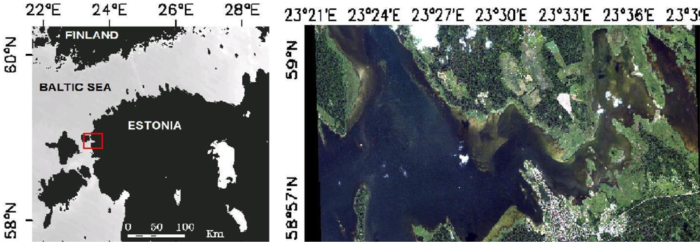
2.1. Study Area
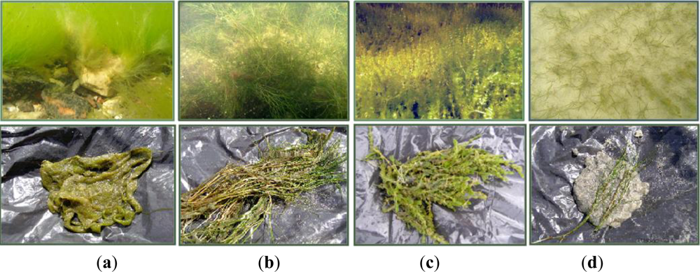
2.2. Field Survey
2.3. Spectral Library
2.4. Remote Sensing Data
2.4.1. CASI
2.4.2. WorldView-2
2.4.3. Classification
3. Results
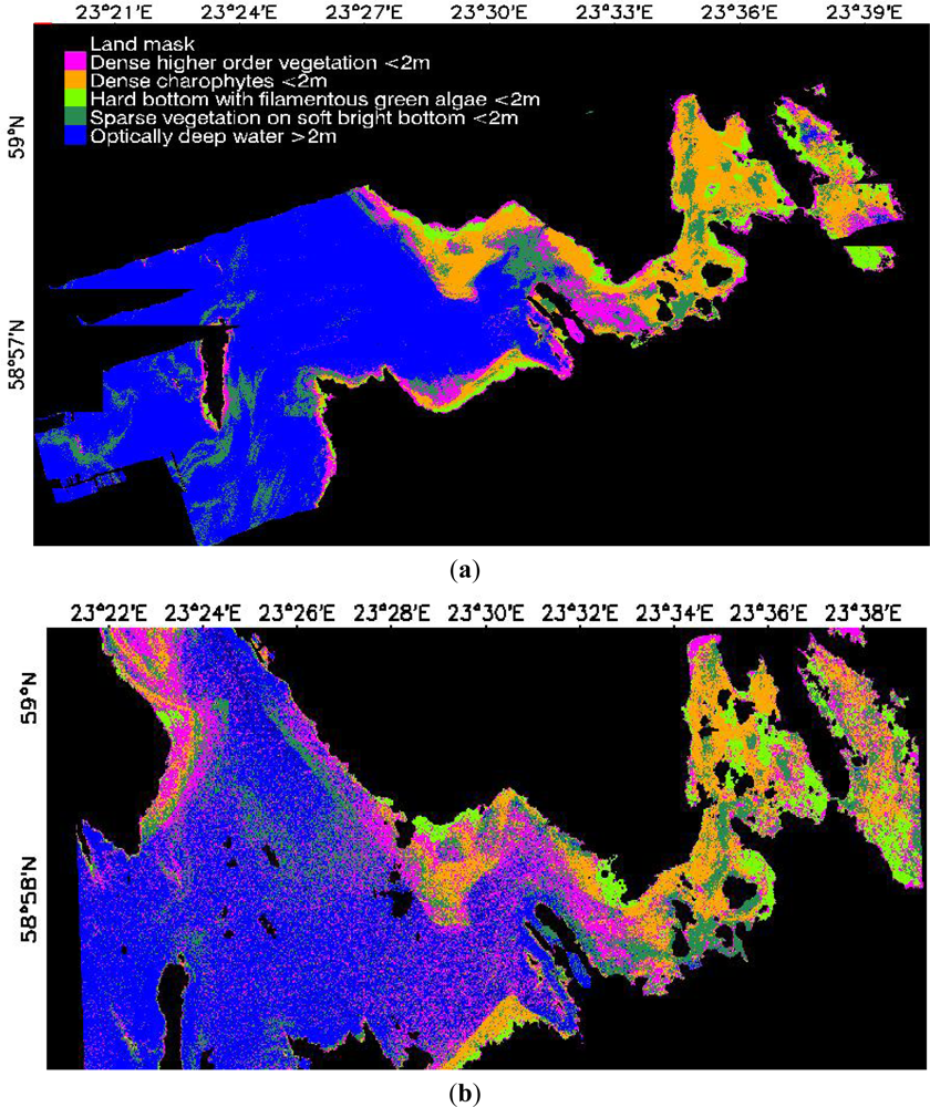
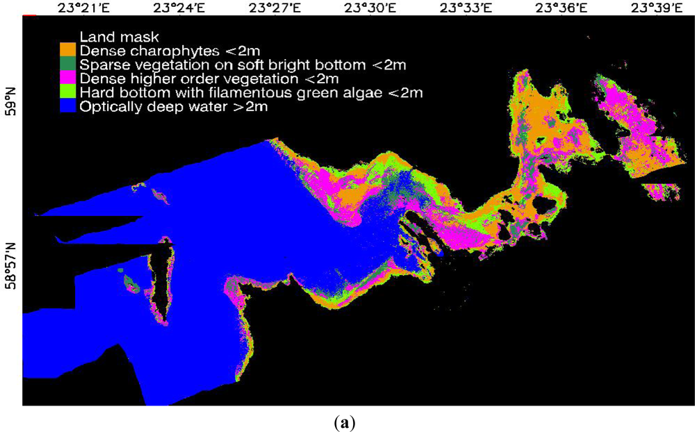
3.1. Image-Based Classification
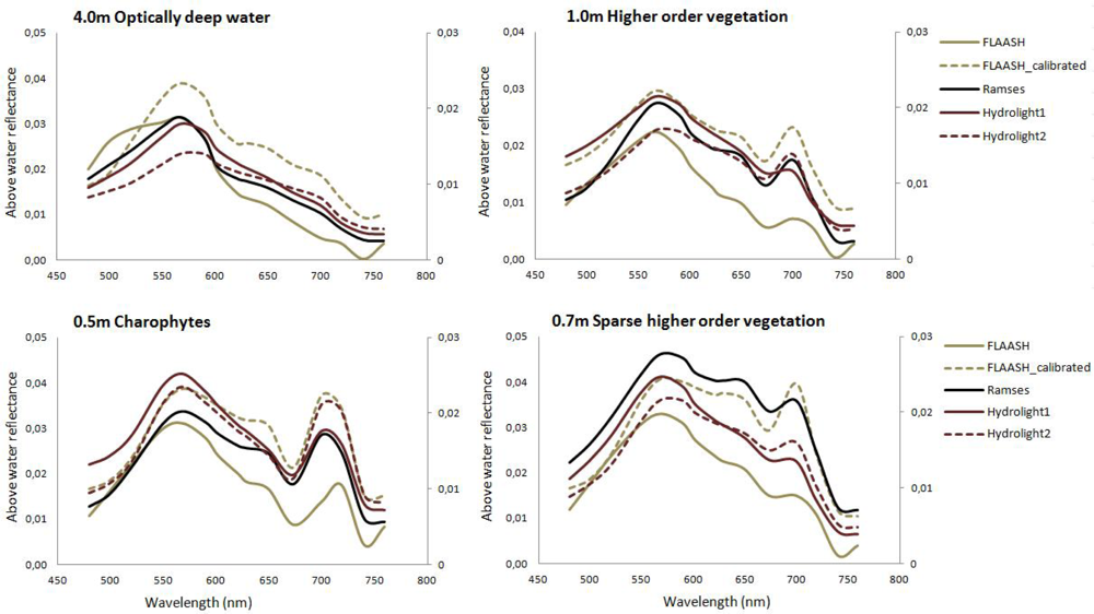
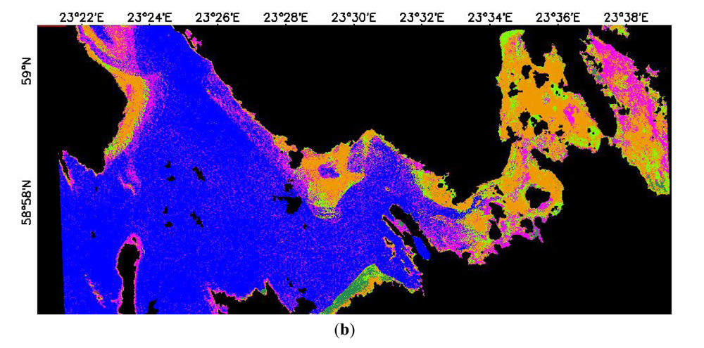
3.2. Spectral Library Classification
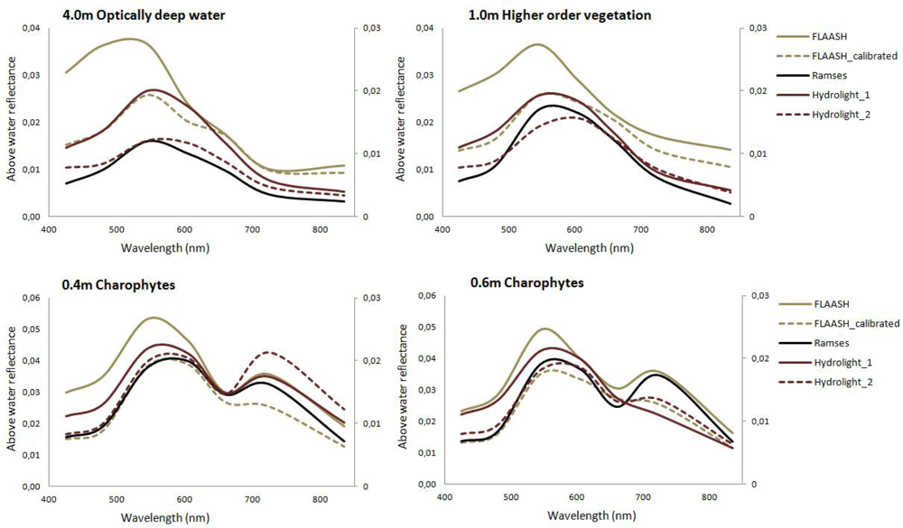
3.2.1. Atmospheric Correction
3.2.2. Classification
4. Discussion
5. Conclusions
Acknowledgments
References
- HELCOM. Ecosystem Health of the Baltic Sea 2003–2007. HELCOM Initial Holistic Assessment. Baltic Sea Environment Proceedings No. 122; Helsinki Commission: Helsinki, Finland, 2010. Available online: http://www.helcom.fi/stc/files/Publications/Proceedings/bsep122.pdf (accessed on 15 December 2012).
- Kotta, J.; Paalme, T.; Martin, G.; Mäkinen, A. Major changes in macroalgae community composition affect the food and habitat preference of Idotea baltica. Int. Rev. Hydrobiol 2000, 85, 693–701. [Google Scholar]
- Torn, K.; Krause-Jensen, D.; Martin, G. Present and past depth distribution of bladderwrack (Fucus vesiculosus) in the Baltic Sea. Aquat. Bot 2006, 84, 53–62. [Google Scholar]
- Thomsen, M.; Wernberg, T.; Engelen, A.; Tuya, F.; Vanderklift, M.; Holmer, M.; McGlathery, K.; Arenas, F.; Kotta, J.; Silliman, B. A meta-analysis of seaweeds impact on seagrasses: generalities and knowledge gaps. PLoS ONE 2012, 7, e28595. [Google Scholar]
- Kotta, J.; Aps, R.; Orav-Kotta, H. Bayesian Inference for Predicting Ecological Water Quality under Different Climate Change Scenarios. In Management of Natural Resources, Sustainable Development and Hazards II; WIT Press: Sussex, UK, 2009. [Google Scholar]
- Phinn, S.R.; Dekker, A.G.; Brando, V.E.; Roelfsema, C.M. Mapping water quality and substrate cover in optically complex coastal and reef waters: An integrated approach. Mar. Pollut. Bull 2005, 51, 459–469. [Google Scholar]
- Malthus, T.J.; Karpouzli, E. Integrating field and high spatial resolution satellitebased methods for monitoring shallow submersed aquatic habitats in the Sound of Eriskay, Scotland, UK. Int. J. Remote Sens 2003, 24, 2585–2593. [Google Scholar]
- Darecki, M.; Stramski, D. An evaluation of MODIS and SeaWiFS bio-optical algorithms in the Baltic Sea. Remote Sens. Environ 2004, 89, 326–350. [Google Scholar]
- Kutser, T.; Paavel, B.; Metsamaa, L; Vahtmäe, E. Mapping coloured dissolved organic matter concentration in coastal waters. Int. J. Remote Sens 2009, 30, 5843–5849. [Google Scholar]
- Kutser, T.; Metsamaa, L.; Vahtmäe, E.; Aps, R. Operative monitoring of the extent of dredging in coastal ecosystems using MODIS satellite imagery. J. Coastal Res. 2007, SI50, 180–184. [Google Scholar]
- Kutser, T.; Metsamaa, L.; Strömbeck, N.; Vahtmäe, E. Monitoring cyanobacterial blooms by satellite remote sensing. Estuar. Coast. Shelf Sci 2006, 67, 303–312. [Google Scholar]
- Vahtmäe, E.; Kutser, T.; Kotta, J.; Pärnoja, M. Detecting patterns and changes in a complex benthic environment of the Baltic Sea. J. Appl. Remote Sens 2011, 5, 053559. [Google Scholar]
- Dekker, A.G.; Brando, V.E.; Anstee, J.M. Retrospective seagrass hange detection in a shallow coastal tidal Australian lake. Remote Sens. Environ 2005, 97, 415–433. [Google Scholar]
- Kutser, T.; Miller, I.; Jupp, D.L.B. Mapping coralreef benthic substrates using hyperspectral space-borne images and spectral libraries. Estuar. Coast. Shelf Sci 2006, 70, 449–460. [Google Scholar]
- Phinn, S.; Roelfsema, C.; Dekker, A.; Brando, V.; Anstee, J. Mapping seagrass species, cover and biomass in shallow waters: An assessment of satellite multi-spectral and airborne hyper-spectral imaging systems in Moreton Bay (Australia). Remote Sens. Environ 2008, 112, 3413–3425. [Google Scholar]
- Bertels, L.; Vanderstraete, T.; Van Coillie, S.; Knaeps, E.; Sterckx, S.; Goossens, R; Deronde, B. Mapping of coral reefs using hyperspectral CASI data; A case study: Fordata, Tanimbar, Indonesia. Int. J. Remote Sens 2008, 29, 2359–2391. [Google Scholar]
- Fearns, P.R.C.; Klonowski, W.; Babcock, R.C.; England, P.; Phillips, J. Shallow water substrate mapping using hyperspectral remote sensing. Cont. Shelf Res 2011, 31, 1249–1259. [Google Scholar]
- Lyons, M.; Phinn, S.; Roelfsema, C. Integrating QuickBird multi-spectral satellite and field data: mapping bathymetry, seagrass cover, seagrass species and change in Moreton Bay, Australia in 2004 and 2007. Remote Sens 2011, 3, 42–64. [Google Scholar]
- Mumby, P.J.; Edwards, A.J. Mapping marine environments with IKONOS imagery: Enhanced spatial resolution can deliver greater thematic accuracy. Remote Sens. Environ 2002, 82, 248–257. [Google Scholar]
- Andrefouet, S.; Kramer, P.; Torres-Pulliza, D.; Joyce, K.E.; Hochberg, E.J.; Garza-Perez, R.; Mumby, P.J.; Riegl, B.; Yamano, H.; White, W.H.; et al. Multi-site evaluation of IKONOS data for classification of tropical coral reef environments. Remote Sens. Environ 2003, 88, 128–143. [Google Scholar]
- Call, K.A.; Hardy, J.T.; Wallin, D.O. Coral reef habitat discrimination using multivariate spectral analysis and satellite remote sensing. Int. J. Remote Sens 2003, 24, 2627–2639. [Google Scholar]
- Wolter, P.T.; Johnston, C.A.; Niemi, G.J. Mapping submerged aquatic vegetation in the US Great Lakes using Quickbird satellite data. Int. J. Remote Sens 2005, 26, 5255–5274. [Google Scholar]
- Pasqualini, V.; Pergent-Martini, C.; Pergent, G.; Agreil, M.; Skoufas, G.; Sourbes, L.; Tsirika, A. Use of SPOT 5 for mapping seagrasses: An application to Posidonia oceanica. Remote Sens. Environ 2005, 94, 39–45. [Google Scholar]
- Fornes, A.; Basterretxea, G.; Orfila, A.; Jordi, A.; Alvarez, A.; Tintore, J. Mapping Posidonia oceanica from IKONOS. ISPRS J. Photogranmm 2006, 60, 315–322. [Google Scholar]
- Theriault, C.; Scheibling, R.; Hatcher, B.; Jones, W. Mapping the distribution of an invasive marine alga (Codium fragile spp. tomentosoides) in optically shallow coastal waters using the compact airborne spectrographic imager (CASI). Can. J. Remote Sens 2006, 32, 315–329. [Google Scholar]
- Gagnon, P.; Scheibling, R.E.; Jones, W.; Tully, D. The role of digital bathymetry in mapping shallow marine vegetation from hyperspectral image data. Int. J. Remote Sens 2008, 29, 879–904. [Google Scholar]
- Schowengerdt, R.A. Remote Sensing Models and Methods for Image Processing; Academic Press: Burlington, MA, USA, 1997. [Google Scholar]
- Chen, D.M.; Stow, D. The effect of training strategies on supervised classification at different spatial resolutions. Photogramm. Eng. Remote Sensing 2002, 68, 1155–1161. [Google Scholar]
- Campbell, J.B. Introduction to Remote Sensing, 4th ed.; The Guilford Press: New York, NY, USA, 2007. [Google Scholar]
- Louchard, E.M.; Reid, R.P.; Stephens, F.C.; Davis, C.O.; Leathers, R.A.; Downes, T.V. Optical remote sensing of benthic habitats and bathymetry in coastal environments at Lee Stocking Island, Bahamas: A comparative spectral classification approach. Limnol. Oceanogr 2003, 48, 511–521. [Google Scholar]
- Lesser, M.P.; Mobley, C.D. Bathymetry, water optical properties, and benthic classification of coral reefs using hyperspectral remote sensing imagery. Coral Reefs 2007, 26, 819–829. [Google Scholar]
- Jaanus, A. Phytoplankton in Estonian Coastal Waters: Variability, Trends and Response to Environmental Pressures. Biologicae Universitatis Tartuensis, Tartu University, Tartu, Estonia, 2011. [Google Scholar]
- Kotta, J.; Jaanus, A.; Kotta, I. Haapsalu and Matsalu Bays. In Ecology of Baltic Coastal Waters; Schiewer, U., Ed.; Springer-Verlag: Berlin/Heidelberg, Germany, 2008; Chapter 11; pp. 245–258. [Google Scholar]
- Kovtun, A.; Torn, K.; Kotta, J. Long-term changes in a northern Baltic macrophyte community. Estonian J. Ecol 2009, 58, 270–285. [Google Scholar]
- Möller, T.; Kotta, J; Martin, G. Effect of observation method on the perception of community structure and water quality in a brackish water ecosystem. Marine Ecol 2009, 30, 105–112. [Google Scholar]
- Morel, A.; Gentili, B. Diffuse reflectance of oceanic waters. II Bidirectional aspects. Appl. Opt 1993, 32, 6864–6879. [Google Scholar]
- Mobley, C.D.; Sundman, L.K. HydroLight 5, Ecolight 5 Users Guide; Sequoia Scientific Inc.: Bellevue, WA, USA, 2008. [Google Scholar]
- Holden, H.; LeDrew, E. Measuring and modeling water column effects on hyperspectral reflectance in a coral reef environment. Remote Sens. Environ 2002, 81, 300–308. [Google Scholar]
- Hedley, J.D.; Harborne, A.R.; Mumby, P.J. Simple and robust removal of sun glint for mapping shallow-water benthos. Int. J. Remote Sens 2005, 26, 2107–2112. [Google Scholar]
- Adler-Golden, S.M.; Matthew, M.W.; Bernstein, L.S.; Levine, R.Y.; Berk, A.; Richtsmeier, S.C.; Acharya, P.K.; Anderson, G.P.; Felde, G.; Gardner, J.; et al. Atmospheric correction for shortwave spectral imagery based on MODTRAN4. Proc. SPIE 1999, 3753, 61–69. [Google Scholar]
- DigitalGlobe Inc. The Benefits of the 8 Spectral Bands of WorldView-2. White Paper; 2010. Available online: www.digitalglobe.com (accessed on 25 March 2013).
- Kruse, F.A.; Dwyer, J.L. The Effect of AVIRIS Atmospheric Calibration Methodology on Identification and Quantification Mapping of Surface Mineralogy, Drums Mountain, Utah. In Proceedings of the 4th JPL Airborne Geoscience Workshop, Washington, DC, USA, 25–29 October 1993; pp. 101–104.
- Vahtmäe, E.; Kutser, T.; Kotta, J.; Pärnoja, M.; Möller, T.; Lennuk, L. Mapping Baltic Sea shallow water environments with airborne remote sensing. Okeanology 2012, 52, 870–876. [Google Scholar]
- Lillesand, T.M.; Kiefer, R.W.; Chipman, J.W. Remote Sensing and Image Interpretation; John Wiley & Sons: New York, NY, USA, 2007. [Google Scholar]
- Kutser, T.; Hiire, M.; Metsamaa, L.; Vahtmäe, E.; Paavel, B.; Aps, R. Field measurements of spectral backscattering coefficient of the Baltic Sea and boreal lakes. Boreal Environ. Res 2009, 14, 305–312. [Google Scholar]
- Metsamaa, L.; Kutser, T.; Strömbeck, N. Recognising cyanobacterial blooms based on their optical signature: a modelling study. Boreal Environ. Res 2006, 11, 493–506. [Google Scholar]
- Nobel, P.S. Physicochemical and Environemntal Plant Physiology, 4th ed.; Elsevier Inc: Oxford, UK, 2009. [Google Scholar]
- Kutser, T.; Vahtmäe, E.; Paavel, P.; Kauer, T. Removing glint effets from field radiometry data measured in optically complex coastal and inland waters. Remote Sens. Environ 2013, 133, 85–89. [Google Scholar]
- Belluco, E.; Camuffo, M.; Ferrari, S.; Modenese, L.; Silvestri, S.; Marani, A.; Marani, M. Mapping salt-marsh vegetation by multispectral and hyperspectral remote sensing. Remote Sens. Environ 2006, 105, 54–67. [Google Scholar]
- Hochberg, E.J.; Atkinson, M.J. Capabilities of remote sensors to classify coral, algae, and sand as pure and mixed spectra. Remote Sens. Environ 2003, 85, 174–189. [Google Scholar]
- Andrefouet, S.; Payri, C.; Hochberg, E.J.; Hu, C.; Atkinson, M.J.; Muller-Karger, F.E. Use of in situ and airborne reflectance for scaling-up spectral discrimination of coral reef macroalgae from species to communities. Marine Ecol. Progr. Series 2004, 283, 161–177. [Google Scholar]
- Kutser, T.; Vahtmäe, E.; Metsamaa, L. Spectral library of macrolagae and benthic substrates in Estonian coastal waters. Proc. Estonian Acad. Sci. Biol. Ecol 2006, 55, 329–340. [Google Scholar]
- Foody, G. On the compensation for chance agreement in image classification accuracy assessment. Photogramm. Eng. Remote Sensing 1992, 58, 1459–1460. [Google Scholar]
- Rosenfield, G.; Fitzpatrick-Lins, K. A Coefficient of agreement as a measure of thematic classification accuracy. Photogramm. Eng. Remote Sensing 1986, 52, 223–227. [Google Scholar]
- Giardino, C.; Bartoli, M.; Candiani, G.; Bresciani, M.; Pellegrini, L. Recent changes in macrophyte colonisation patterns: An imaging spectrometry-based evaluation of southern Lake Garda (northern Italy). J. Appl. Remote Sens 2007, 1, 011509. [Google Scholar]
- Williams, D.J.; Rybicki, N.B.; Lombana, A.V.; O’Brien, T.M.; Gomez, R.B. Preliminary investigation of submerged aquatic vegetation mapping using hyperspectral remote sensing. Environ. Monit. Assess 2003, 81, 383–392. [Google Scholar]
- Mishra, D.; Narumalani, S.; Rundquist, D.; Lawson, M.; Perk, R. Enhancing the detection and classification of coral reef and associated benthic habitats: A hyperspectral remote sensing approach. J. Geophys. Res 2007, 112, C08014. [Google Scholar]
- Lyons, M.; Phinn, S.; Roelfsema, C. Integrating QuickBird multi-spectral satellite and field data: Mapping bathymetry, seagrass cover, seagrass species and change in Moreton Bay, Australia in 2004 and 2007. Remote Sens 2011, 3, 42–64. [Google Scholar]
- Kutser, T.; Pierson, C.D.; Kallio, K.Y.; Reinart, A.; Sobek, S. Mapping lake CDOM by satelliite remonte sensing. Remote Sens. Environ 2006, 94, 535–540. [Google Scholar]
- Kutser, T. Quantitative detection of chlorophyll in cyanobacterial blooms by satelliite remonte sensing. Limnol. Oceanogr 2004, 49, 2179–2189. [Google Scholar]
- O’Neill, J.D.; Costa, M.; Sharma, T. Remote sensing of shallow coastal benthic substrates: In situ spectra and mapping of eelgrass (Zostera marina) in the Gulf Islands National Park Reserve of Canada. Remote Sens 2011, 3, 975–1005. [Google Scholar]
- Vahtmae, E.; Kutser, T.; Martin, G.; Kotta, J. Feasibility of hyperspectral remote sensing for mapping benthic macroalgal cover in turbid coastal waters—A Baltic Sea case study. Remote Sens. Environ 2006, 101, 342–351. [Google Scholar]
- Kruse, F.; Lefkoff, A.; Boardman, A.B.; Heidebrecht, K.B.; Shapiro, A.T.; Barloon, P.J.; Goetz, A.F.H. The Spectral Image Processing System (SIPS) dinteractive visualization and analysis of imaging spectrometer data. Remote Sens. Environ 1993, 44, 145–163. [Google Scholar]
- Kutser, T.; Vahtmäe, E.; Praks, J. A sun glint correction method for hyperspectral imagery containing areas with non-negligible water leaving NIR signal. Remote Sens. Environ 2009, 113, 2267–2274. [Google Scholar]
- Kay, S.; Hedley, J.D.; Lavender, S. Sun glint correction of high and low spatial resolution images of aquatic scenes: A review of methods for visible and near-infrared wavelengths. Remote Sens 2009, 1, 697–730. [Google Scholar]
- Mobley, C.D.; Sundman, L.K; Davis, C.O.; Bowles, J.H.; Downes, T.V.; Leathers, R.A.; Montes, M.J.; Bissett, W.P.; Kohler, D.D.; Reid, R.P.; et al. Interpretation of hyperspectral remote-sensing imagery by spectrum matching and look-up tables. Appl Opt 2005, 44, 3576–3592. [Google Scholar]
- Dekker, A.G.; Phinn, S.R.; Anstee, J.; Bissett, P.; Brando, V.E.; Casey, B.; Fearns, P.; Hedley, J.; Klonowski, W.; Lee, Z.P.; et al. Intercomparison of shallow water bathymetry, hydro-optics, and benthos mapping techniques in Australian and Caribbean coastal environments. Limnol. Oceanogr.: Methods 2011, 9, 396–425. [Google Scholar]
- Casal, G.; Kutser, T.; Dominguez-Gomez, J.A.; Sanchez-Carnero, N.; Freire, J. Mapping benthic macroalgal communities in the coastal zone using CHRIS-PROBA mode 2 images. Estuarine Coastal Shelf Sci 2011, 94, 281–290. [Google Scholar]
- Casal, G.; Sanchez-Carnero, N.; Dominguez-Gomez, J.A.; Kutser, T.; Freire, J. Assessment of AHS (Airborne Hyperspectral Scanner) sensor to map macroalgal communities on the Ria de vigo and Ria de Aldan coast (NW Spain). Mar. Biol 2012, 159, 1997–2013. [Google Scholar]
- Hestir, E.L.; Khanna, S.; Andrew, M.E.; Santos, M.J.; Viers, J.H.; Greenberg, J.A.; Rajapakse, S.S.; Ustin, S.L. Identification of invasive vegetation using hyperspectral remote sensing in the California Delta ecosystem. Remote Sens. Environ 2008, 112, 4034–4047. [Google Scholar]


| Water Type | CChl | CSM | aCDOM(380) |
|---|---|---|---|
| 1 | 2.65 | 4.40 | 2.03 |
| 2 | 6.39 | 3.20 | 4.61 |
| Band | Wavelength (nm) | Band | Wavelength (nm) |
|---|---|---|---|
| 1 | 367.6–372.4 | 14 | 646.9–651.7 |
| 2 | 396.2–401.0 | 15 | 670.7–675.5 |
| 3 | 436.8–441.6 | 16 | 697.0–701.8 |
| 4 | 455.9–460.7 | 17 | 716.1–720.9 |
| 5 | 477.4–482.2 | 18 | 737.5–742.3 |
| 6 | 496.5–501.3 | 19 | 756.6–761.4 |
| 7 | 517.9–522.7 | 20 | 775.7–782.9 |
| 8 | 546.6–551.4 | 21 | 816.3–821.1 |
| 9 | 565.7–570.5 | 22 | 835.4–840.2 |
| 10 | 587.2–592.0 | 23 | 875.4–882.6 |
| 11 | 599.1–603.9 | 24 | 935.5–942.7 |
| 12 | 618.2–623.0 | 25 | 1,035.7–1,054.7 |
| 13 | 625.4–632.6 |
| Overall Accuracy | Kappa Coefficient | |
|---|---|---|
| CASI image-based classification | 77.5% | 0.70 |
| CASI spectral library classification (FLAASH) | 57.5% | 0.43 |
| CASI spectral library classification (FLAASH calibrated) | 70.8% | 0.61 |
| WV-2 image-based classification | 71.6% | 0.62 |
| WV-2 spectral library classification (FLAASH) | 64.6% | 0.52 |
| WV-2 spectral library classification (FLAASH calibrated) | 63.5% | 0.53 |
© 2013 by the authors; licensee MDPI, Basel, Switzerland This article is an open access article distributed under the terms and conditions of the Creative Commons Attribution license ( http://creativecommons.org/licenses/by/3.0/).
Share and Cite
Vahtmäe, E.; Kutser, T. Classifying the Baltic Sea Shallow Water Habitats Using Image-Based and Spectral Library Methods. Remote Sens. 2013, 5, 2451-2474. https://doi.org/10.3390/rs5052451
Vahtmäe E, Kutser T. Classifying the Baltic Sea Shallow Water Habitats Using Image-Based and Spectral Library Methods. Remote Sensing. 2013; 5(5):2451-2474. https://doi.org/10.3390/rs5052451
Chicago/Turabian StyleVahtmäe, Ele, and Tiit Kutser. 2013. "Classifying the Baltic Sea Shallow Water Habitats Using Image-Based and Spectral Library Methods" Remote Sensing 5, no. 5: 2451-2474. https://doi.org/10.3390/rs5052451