Geometric Accuracy Investigations of SEVIRI High Resolution Visible (HRV) Level 1.5 Imagery

Abstract

GCOS (Global Climate Observing System) is a long-term program for monitoring the climate, detecting the changes, and assessing their impacts. Remote sensing techniques are being increasingly used for climate-related measurements. Imagery of the SEVIRI instrument on board of the European geostationary satellites Meteosat-8 and Meteosat-9 are often used for the estimation of essential climate variables. In a joint project between the Swiss GCOS Office and ETH Zurich, geometric accuracy and temporal stability of 1-km resolution HRV channel imagery of SEVIRI have been evaluated over Switzerland. A set of tools and algorithms has been developed for the investigations. Statistical analysis and blunder detection have been integrated in the process for robust evaluation. The relative accuracy is evaluated by tracking large numbers of feature points in consecutive HRV images taken at 15-minute intervals. For the absolute accuracy evaluation, lakes in Switzerland and surroundings are used as reference. 20 lakes digitized from Landsat orthophotos are transformed into HRV images and matched via 2D translation terms at sub-pixel level. The algorithms are tested using HRV images taken on 24 days in 2008 (2 days per month). The results show that 2D shifts that are up to 8 pixels are present both in relative and absolute terms.

1. Introduction

1.1. Motivation and Background

GCOS (Global Climate Observing System) is a long-term program for monitoring the climate, detect the changes, and assess their impacts. It is undertaken by several international organizations, such as WMO, IOC, UNESCO, UNEP and ICSU [1]. The Swiss GCOS Office at the Federal Office of Meteorology and Climatology MeteoSwiss is responsible for coordinating GCOS activities in Switzerland [2].

Remote sensing techniques and satellite imagery are being increasingly used for climate-related measurements. The number of satellites suitable for meteorological applications is growing steadily, and the geometric, radiometric, spectral and temporal resolutions of their sensors are constantly improving, allowing the extraction of new, additional information or an improved determination of current parameters. Satellites are particularly suited for the widespread, repetitive observations of the Earth, even over areas that are difficult to access [3,4].

Accurate georeferencing of satellite imagery is important for generation of fundamental climate data records (FCDR) from satellite observations, in order to avoid errors due to misregistration. An example on the impact of band-to-band misregistration errors for MODIS Aqua can be found in [5]. GCOS has also defined target requirements for geometric accuracy [4].

So far, the main focus has been on radiometric accuracy, and less attention has been paid on the geometric accuracy. A research project is carried out by the Photogrammetry and Remote Sensing Group at the ETH Zurich in the framework of an agreement with the Swiss GCOS Office at MeteoSwiss. The project aims at analyzing the geometric accuracy of three commonly used satellite sensors over Switzerland: SEVIRI (on board of the European meteorological satellites Meteosat-8 and Meteosat-9), MODIS (on board of the NASA satellites Terra and Aqua), and AVHRR (on board of the NOAA and Metop satellite series). It includes the following activities:

(a)

Investigation of the relative geometric accuracy within one image, between different channels, and for multi-temporal imagery;

(b)

Investigation of the absolute geometric accuracy using reference data;

(c)

Investigation of the temporal stability of the absolute as well as the relative geometric accuracy (e.g., from different orbital overpasses, in case of satellite maneuvers, etc.);

(d)

First analysis of the impact of geometric errors on the derivation of climate parameters.

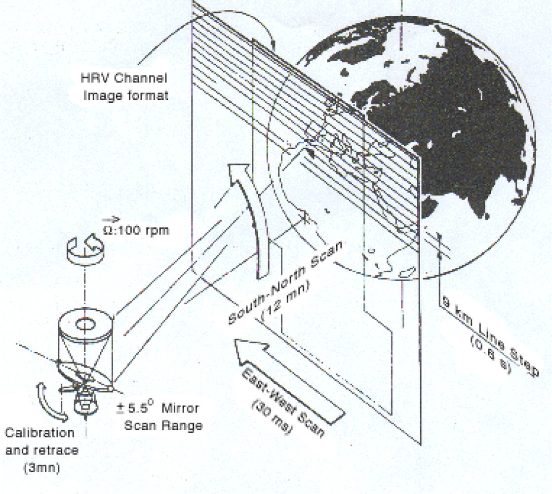
In the first stage of the project, the relative and the absolute geometric accuracies of the HRV (High-Resolution Visible) channel imagery of SEVIRI (Spinning Enhanced Visible and Infra-Red Imager) have been investigated. The SEVIRI instruments acquire images on board of the Meteosat-8 (formerly MSG-1) and Meteosat-9 (formerly MSG-2) satellites. In order to achieve the project goals, a set of algorithms has been developed and implemented. The algorithms can determine the relative and absolute accuracies of HRV Level 1.5 at sub-pixel level. In addition, they allow fully-automatic processing of massive amounts of data (e.g., all images of a year).

There have been a few studies in the literature reporting the geometric accuracy of the SEVIRI imagery. Hanson et al. [6] conducted some tests on the absolute and relative geometric accuracies of the SEVIRI aboard the Meteosat-8 during the commissioning phase. The results were mainly obtained from the Image Quality Ground Support Equipment (IQGSE), with a remark that comparable results are expected from the image processing system that is used for routine operations, called IMPF. The IQGSE identifies landmarks (coastlines) in the Level 1.5 image and derives statistics from their expected and their actual position. They have reported that the geometric performances meet the specifications, usually with a significant margin. They have also performed tests during the eclipse and maneuver times. One maneuver case is analyzed and the results indicate that it should be possible to meet the outage specification [6].

Hanson and Müller [7] have reported an East-West image shift immediately after eclipse up to 3 pixels with respect to the multispectral (MS) channels of Meteosat-8 with 3 km nominal resolution. Gieske et al. [8] have reported that the geocoding accuracy for Meteosat-8 is typically in the order of 1 pixel for the MS imagery. However, in the analysis of image time series it was also noted that sometimes shifts are observed. Dürr and Zelenka [9] have used HRV and MS images that are acquired between 2004 and 2006 from Meteosat-8 and Meteosat-9 in their study and improved the geolocation of the HRV imagery. They have applied a similar approach as proposed here, and used lakes in order to compute shifts at pixel level accuracy on the HRV images over Alpine areas. They have observed shifts up to 8 pixels to the North.

1.2. MSG-SEVIRI

Meteosat Second Generation (MSG) is a series of 4 geostationary satellites developed and procured by the European Space Agency (ESA) on behalf of the European Organization for the Exploitation of Meteorological Satellites (EUMETSAT). SEVIRI is the main instrument carried aboard the Meteosat-8 and Meteosat-9, which are positioned above the equator at longitudes of 9.6°E and 0.0°W, respectively [10]. In operational service, the SEVIRI aboard the Meteosat-9 provides very high temporal resolution and scans the complete disk of the Earth with a 15 min repeat cycle. Meteosat-8 is used as stand-by, and scans a sub region with a 5 min repeat cycle in Rapid Scan Mode [10].

The SEVIRI instrument is designed to support nowcasting, numerical weather forecasting, and climate applications over Europe and Africa [11]. It combines the East-West scan generated by the satellite spin motion and the South to North micro-step scan of a mirror. The imaging phase takes twelve minutes, and the remaining three minutes are allocated for calibration, retrace and stabilization. Figure 1 shows the Earth imaging principle used by SEVIRI. The instrument generates images of the Earth in 12 different spectral channels, from visible to infrared (

Table 1. SEVIRI channel characteristics [12].

Channel ID	Absorption Band/Channel Type	Spectral Bandwidth (m)	Spectral Bandwidth As % of energy actually detected within spectral band
HRV	Visible/High Resolution	0.6 to 0.9	Precise spectral characteristics not critical
VIS 0.6	VNIR/Core Imager	0.56 to 0.71	98.0 %
VIS 0.8	VNIR/Core Imager	0.74 to 0.88	99.0 %
IR 1.6	VNIR/Core Imager	1.50 to 1.78	99.0 %
IR 3.9	IR/Window Core Imager	3.48 to 4.36	98.6 % (1)
IR 6.2	Water Vapour/Core Imager	5.35 to 7.15	99.0 %
IR 7.3	Water Vapour/Pseudo-Sounding	6.85 to 7.85	98.0 %
IR 8.7	IR/Window Core Imager	8.30 to 9.10	98.0 %
IR 9.7	IR/Ozone Pseudo-Sounding	9.38 to 9.94	99.0 %
IR 10.8	IR/Window Core Imager	9.80 to 11.80	98.0 %
IR 12.0	IR/Window Core Imager	11.00 to 13.00	98.0 %
IR 13.4	IR/Carbon Dioxide	12.40 to 14.40	96.0 %
	Pseudo-Sounding

). For the HRV channel, there are nine detectors, and nine lines are obtained per satellite revolution at 1 km resolution (nominal at Sub Satellite Point, SSP). The HRV images are acquired on a reduced Earth area and have the spectral bandwidth of 0.6–0.9 μm [12]. EUMETSAT corrects the raw Level 1.0 image in real-time for all radiometric and geometric effects and georeferences it using a standardized projection [12]. The resulting Level 1.5 image consists of georeferenced, calibrated and radiance-linearized information for the derivation of meteorological products and other further meteorological processing [12,13]. Geometric accuracy expectations for SEVIRI Level 1.5 data acquired from Meteosat-8 and Meteosat-9 are provided by EUMETSAT [14] and shown in

Table 2. Geometric rectification accuracy specification and performances of SEVIRI level 1.5 data provided by the European Organization for the Exploitation of Meteorological Satellites (EUMETSAT) [14].

Geometric Quality Criterion	Specification (km SSP/Pixel Size at SSP)	Meteosat-8/9 Performance (km)
Absolute accuracy	<3.0 (3 pixels for HRV)	1.2
Relative accuracy between two consecutive images	<1.2 (3 pixels for HRV)	0.3
Relative accuracy within an image (over 500 samples)	<3.0 (3 pixels for HRV)	1.2

.

EUMETSAT Central Operations Reports for 2008 [15,16] point out several geometric problems in the images, which were caused by a number of different reasons (e.g., reduced geometric quality following a North-South Station-Keeping maneuver in February, ground-station-Sun-satellite colinearity in March, Meteosat-9 entering safe-mode on 13 May, RAID array failure on the image processing system on 20-May, etc.). Meteosat-8 currently supports the rapid-scan service covering the latitude range of 15°N to 70°N [16]. However, in case of a satellite/instrument unavailability of Meteosat-9, it is used as the primary mission. As an example, on the 13–14 of May 2008, Meteosat-9 entered safe-mode and Meteosat-8 started to operate as the prime mission. The satellite swap required almost 4 hours and resulted in a loss of 16 Repeat Cycles [16].

2. Data and Methodology

2.1. Data and Software

SEVIRI Level 1.5 data from the year 2008 have been delivered by the Swiss GCOS Office in NetCDF4 format. Since the main aim is to analyze data quality over Switzerland, full HRV images were not used. The used image parts cover a rectangular area over Switzerland and surrounding countries and have a size of 652 × 393 pixels. The ground sample distances (GSD) of the image pixels in the project area vary in the range of 1–2 km. The HRV image part acquired on 30 August 2008 at 12:00 UTC, and all lakes used for absolute accuracy evaluation can be seen in Figure 2. A cloud mask with same spatial resolution is provided for each HRV image. The cloud masks consist of labels for each pixel as; cloud free, thin cloud, and thick cloud. Although the images have been acquired mainly from Meteosat-9, there is a substantial amount of imagery, which has been acquired from Meteosat-8 throughout the year. In addition, there are gaps in the image series for several days, where no data is available.

A stand-alone software package is being implemented in Python 2.6 programming language for highly automatized processing of the SEVIRI data. Python is chosen due to the availability of extensive geospatial, image processing, computer vision and mathematics libraries (e.g., opencv, arcpy, pyproj, pil, etc.). More details and documentation on Python programming language can be found on the Python website [17]. The methods and procedures for relative and absolute accuracy evaluations are described in the following sections.

The data delivered by Meteoswiss are extracted using the NetCDF4 library for Python. The given HRV reflectance values are converted into 8 bit grayscale images by linear stretching. The cloud masks are also transformed into 8 bit images due to technical requirements in the fully automated matching process.

The investigations have been done on the images acquired on 24 different days in 2008. In order to evaluate the temporal stability throughout the year, 2 days from each month are selected for processing. The selection has been done automatically by analyzing the HRV cloud mask obtained from the 12:00 UTC image of each day. Minimum cloud coverage is preferred for the evaluation.

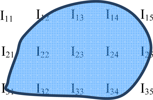
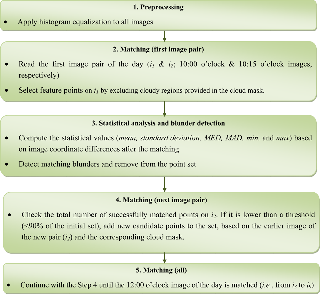
2.2. Relative Accuracy Evaluation

The relative accuracy is evaluated for consecutive HRV images for each day, in order to have very small illumination differences between the images used for matching. For each day, nine images acquired between 10:00 and 12:00 UTC are used for the evaluation. This time frame is selected for the algorithm testing and initial investigations, and will be extended for a more comprehensive analysis in the future. The processing steps for the relative accuracy investigations with the HRV channel data are depicted in Figure 3.

As a first step, histogram equalization is applied to all images in order to increase the contrast and thus the number of points matched. The initial feature points are extracted from the selected first image of the day (10:00) using the goodFeaturesToTrack function in OpenCV [18]. The function finds the most prominent corners in the image, as described in [19]. The given HRV cloud masks are integrated in the feature point selection process in order to exclude cloud regions. The main advantage of using the cloud masks is that it prevents false matches in cloud regions and thus increases the robustness of the whole procedure.

The candidate points are matched in the consecutive image (i.e., taken at 10:15) using the KLT Tracking function of OpenCV (calcOpticalFlowPyrLK). The function matches feature points in an image pair using the Lucas-Kanade method with pyramids [20]. In case of SEVIRI-HRV imagery, no image pyramids are needed due to the small shifts between consecutive images.

After matching of consecutive images, statistical values are calculated for the whole point set based on the image coordinate differences with signs (Δx,Δy) for both axes (x,y): Mean, standard deviation (σ), median (MED), median absolute deviation (MAD) from the median, minimum, and maximum values (formulas are provided in Appendix). Every (Δx,Δy) is compared against the mean-x and mean-y, respectively; and the ones having an absolute difference larger than 3σ are considered as outliers. The blunders usually occur in low contrast and low texture areas and are caused by matching errors. After the removal of outliers, the statistical parameters are recalculated. The outlier check is repeated until a blunder-free set is obtained. The (Δx,Δy) are plotted on a preprocessed reference image for an optional visual assessment of the errors, in terms of location, direction and magnitude.

As described in Steps 4 and 5 in Figure 3, the matching process continues until the last image of the day, which is selected as 12:00 image for this evaluation. The points that are successfully matched (i.e., remaining after the blunder detection) are used as candidate points for the next pair of images (e.g., 10:15 and 10:30). If the total number of points after the blunder detection falls below a given threshold (90% of the point number in the initial image), new points are added to the candidate list based on the earlier image of the new pair and the corresponding cloud mask. In practice, the total number of points is usually above 500 and the percentages of matching outliers are in the range of 3%–20%, with an average of 10%. The spatial distribution of the points in non-cloudy areas is adequate for the relative accuracy evaluation purposes.

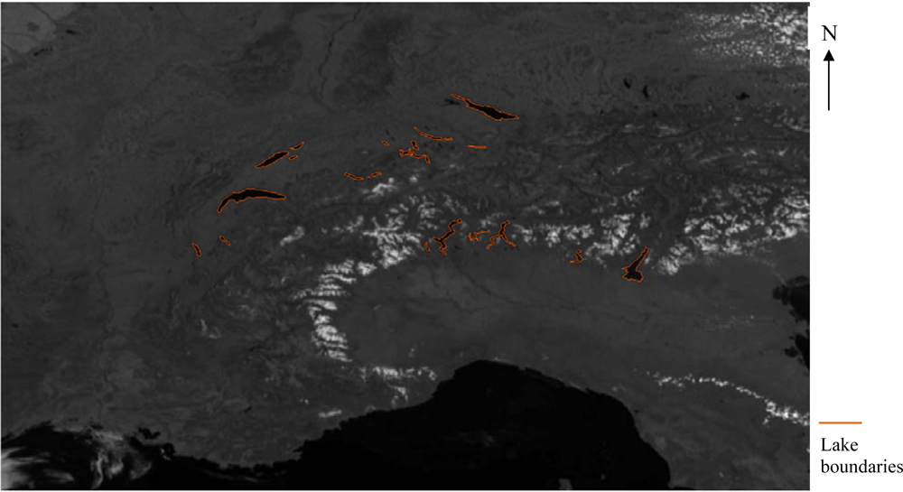
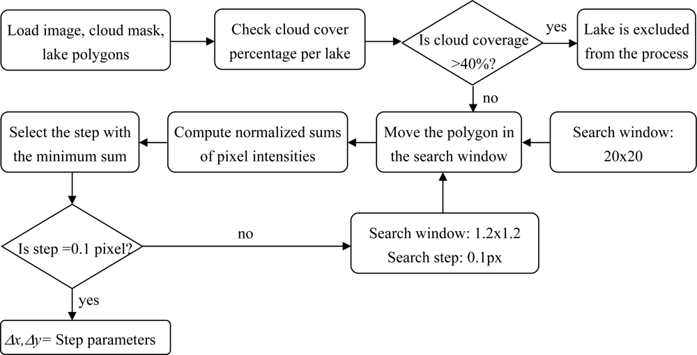
2.3. Absolute Accuracy Evaluation

Absolute accuracy evaluation of the MSG-SEVIRI imagery is done based on lakes, since the detection of shorelines in the HRV images is relatively easy and reliable. The coastlines, which are also visible in the images, have also been considered initially as potential features to be used for the evaluations. The GSHHS (Global self-consistent hierarchical high-resolution shoreline database) has been analyzed for using as reference data [21]. However, the precision of this dataset is between ∼50 and 500 m, which is not sufficient for the evaluation of 1km resolution imagery. Optimally, in photogrammetry, the reference data (ground control points) should have an accuracy of an order of magnitude better than the image GSD, i.e., one-tenth of the GSD, which means 100 m for the HRV imagery. Therefore, only the lake shorelines are used in the process.

The main approach in this study is based on the fact that the pixel grey values of the lakes in the HRV images are low, e.g., less than 30, based on the empirical investigations performed prior to the algorithm development. In addition, the lake pixels are usually darker than the ones of the surrounding areas.

The reference lakes are digitized from two different Landsat orthophotos that are freely available on the Web. The first one is a Landsat 5 image mosaic of Switzerland, which has been produced by Swisstopo [22]. It has been assembled out of about 20 individual images taken by the Landsat 5, in the years 1990 to 1994. Terrain, color and atmospheric corrections are applied on the images. The resulting mosaic is in Swiss Coordinate System (CH1903+) and has a GSD of 25 m. Although the Landsat images have been acquired at much earlier times, no large deviations for the lake areas are observed, when compared with the digital vector maps of Switzerland (VECTOR25).

The second Landsat orthophoto has been available under the Global Land Survey program of USGS [23]. The Landsat 5 image is acquired on 21 August 2011, has a resolution of 30 m, and is in UTM projection system (32°N). This image is only used to extract the Garda Lake, which has a large area and is visible in the HRV images. Since it is only partially covered in the Swiss orthophoto mosaic, it is digitized in the USGS Landsat-5 orthophoto and transformed into the same projection system (Swiss Coordinate System).

The relationship between the geographical and image coordinates of SEVIRI Level 1.5 data is described in a specification document prepared by the Coordination Group for Meteorological Satellites [24]. The main purpose of the document is to define a standard for data dissemination from geostationary satellites. It also provides a set of functions which describes the relation between the geographical coordinates and the image coordinates of each HRV pixel in GEOS (Normalized Geostationary Projection). The GEOS defines the coordinates as Latitude and Longitude on a custom ellipsoid presented in the same document [24]. However, this ellipsoid is assumed to be the same as WGS84 here, since the ellipsoid parameters are similar. An image and ground coordinate transformation software, Navigation Software for MSG-Level 1.5 VIS/IR/HRV data, provided by EUMETSAT [25] is adapted and used in this study.

The preprocessing steps for the absolute geometric accuracy evaluation can be described as following:

• 39 large lakes (except the Garda Lake) in and around Switzerland are digitized manually and saved as vector polygons in Swiss Coordinate System.
• The Garda Lake in Italy is digitized manually on the Landsat 5 orthophoto of USGS and transformed into the Swiss Coordinate System.
• All 40 lakes are first transformed from the Swiss Coordinate System into the GEOS, and then into the HRV image space.
• A cartographic generalization is applied to all lakes to reduce the level of detail of the polygons by removing dense vertices (e.g., forming edges with a length of less than 0.1 pixel).
• After a visual inspection and initial tests for matching, small lakes, which cover an area of smaller than 7 pixels, are removed from the evaluation. The remaining 20 lakes are used for the investigations.

For the matching, each lake polygon is moved inside a 20 × 20 pixels search window (i.e., ± 10 pixels) starting from its initial position. This window size has been found sufficient for the tests. A coarse-to-fine matching is performed at two different steps: firstly, 1 pixel step size is applied to have an approximate matching; and secondly, the results obtained from the first matching are refined by using a window size of 1.2 × 1.2 pixels (i.e., ± 0.6 pixels). For the fine matching, a step size of 0.1 pixel is selected in order to achieve sub-pixel accuracy. At each step, the normalized sum of pixel intensities inside the lake polygons is computed. The partial pixels at the polygon edges are also added to the sum with respect to the pixel area that falls inside the polygon (Figure 4). The coverage area of the lake on a pixel, which is located at the lake edge, is calculated after clipping the lake polygon against pixel boundaries.

The minimum of the normalized sums is selected for each lake within a given image. The step parameters (Δx,Δy), which provides the minimum sum, is considered as the shift of the lake. The algorithm for matching a lake polygon in the HRV image is depicted in Figure 5. The statistical values (mean,σ, MED, MAD, min, max) are derived from the shifts of all lakes in an image. After initial experiments, lakes having a cloud cover percentage of over 40% are excluded from the process since the matching is usually not successful.

3. Results and Discussion

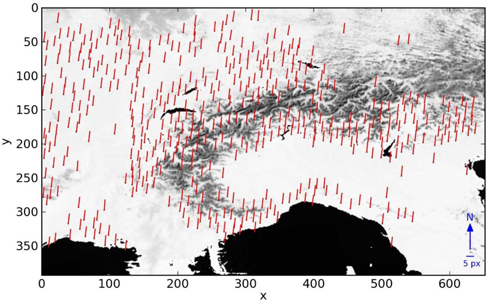
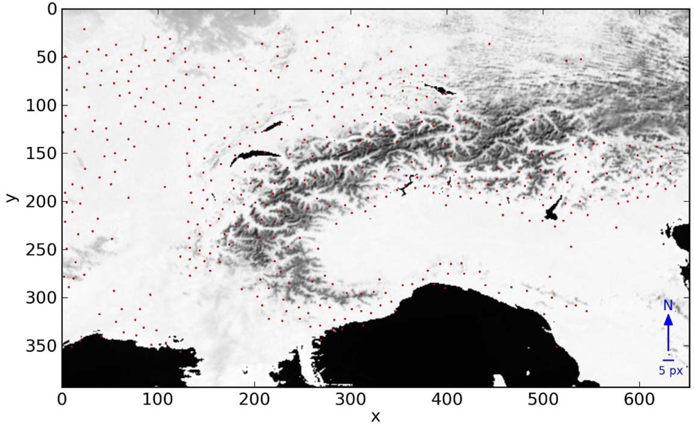
3.1. Relative Accuracy Investigations

A statistical summary of all results obtained from the processing of 216 HRV images acquired on 24 different days (i.e., nine images per day, from 10:00 to 12:00, resulting in 192 image pairs) is given in

Table 3. Relative accuracy evaluation; statistical values of shifts (x) and (y) from all image pairs acquired on 24 different days in the year 2008. All results are given in pixels.

	Mean (x)	Mean (y)	Mean (xy)	MED (x)	MED (y)	σ (x)	σ (y)	MAD (x)	MAD (y)
Min	−0.86	−8.11	0.01	−0.91	−8.11	0.03	0.03	0.02	0.02
Max	1.01	6.90	8.15	0.99	6.92	0.27	0.22	0.13	0.13
Mean	−0.02	0.01	0.46	−0.03	0.01	0.09	0.11	0.05	0.07

. The number of points matched in consecutive image pairs range between 293 and 1003, with an average of 613. The low number of points is mainly due to the high cloud coverage in the corresponding images. The processing time for the matching of all 216 images is only a few minutes on a PC with moderate configuration.

The Min and Max values for the Mean_x and Mean_y, which are presented in Table 3, show that the relative shifts occur in all directions. However, the variations are larger in y axis (up to 8 pixels). The minus sign shows shifts to West and South for x and y, respectively. The Mean and Median values of the shifts are quite similar, showing that no big blunders exist in the results. The standard deviations (σ_x,σ_y) are up to 0.3 pixels, with a mean of 0.1 pixels. The larger σ values (i.e., up to 0.3 pixels) are observed in the images, where small clouds exist in many areas. The Mean σ values can be considered as matching accuracy as well. The MAD can be used as a consistent estimator for the estimation of the standard deviation σ after a multiplication with a constant scale factor, which is 1.48 for normally distributed data (see Appendix as well). The Mean_xy values provided in Table 3 show the errors in terms of 2D distances.

An in depth analysis has been done for 7 February, where large shifts between the images have occurred. The images, which are analyzed here, have been acquired with Meteosat-8. One residual plot obtained from the matching of consecutive images, which were acquired at 10:30 and 10:45, is shown in Figure 6. The total number of candidate points for this matching is 669, and the number of successfully matched points is 591. Mean values of the residuals for x and y are 0.8 and −7.0 pixels, respectively. Both the σ_x and σ_y are 0.1 pixels. Figure 7 shows the residual plot for the same image pair, after removal of the mean shift. The remaining residuals do not show any systematic effect, which implies existence of only 2D shift errors between the images.

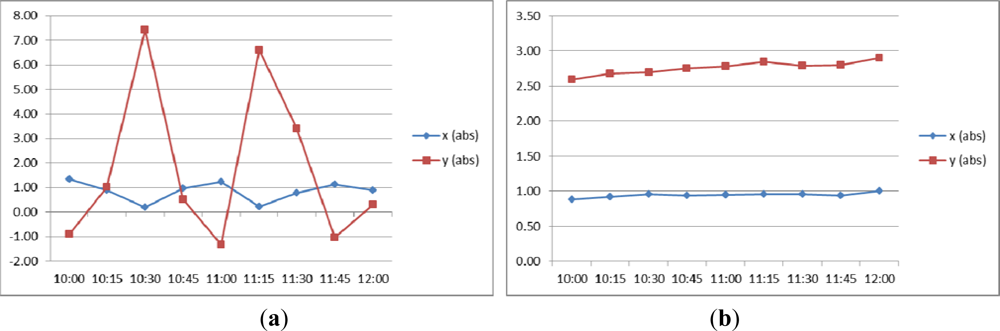
3.2. Absolute Accuracy Investigations

A total of 24 images acquired on 24 different days at 12:00 are processed and the results are summarized in

Table 4. Absolute accuracy evaluation; statistical summary from the shifts of 12:00 images acquired on 24 days in year 2008.

	Shift x (pixel)	Shift y (pixel)	Shift xy (pixel)
Min/Max	0.3/1.5	0.3/3.3	0.9/3.3
Mean/Median	0.9/1.0	2.2/2.2	2.4/2.4
σ/MAD	0.3/0.1	0.6/0.2	0.5/0.2

. The range for the number of lakes used for the evaluations is 6–20, with a mean of 16. The variations are caused due to the exclusion of the lakes, which are largely or completely covered by the clouds, from the process. The processing time for each image varies with respect to the total number of lakes used in the evaluation. Matching of all 20 lakes in an image takes around 15 min. However, not much effort has been invested for the processing time optimization and left as future work.

The statistical values are derived from the estimated shift values of all 24 days. The shifts are shown with signs, where +Δy indicates a shift to the North and +Δx indicates a shift to the East. All 24 images evaluated here are shifted to North and East. The variation in y is larger, between 0.3 to 3.3 pixels, showing poorer stability of the sensor in this direction. The standard deviations calculated from the individual lake offsets in an image range between 0.1 and 0.3 pixels, with a mean standard deviation of 0.2 pixels, which shows the mean accuracy of the matching. This value can as well be interpreted as the variability of absolute accuracy among the lakes of one image. The 2D distances (shift xy) are also provided in Table 4 for the comparison with the sensor geometric accuracy specifications.

An extended analysis has been performed with the data of two different days. Figure 8 shows the absolute accuracy of a total of 18 images acquired with Meteosat-8 and Meteosat-9. Initially, the absolute accuracy values are computed for the 12:00 images of both days with lake matching. The relative shifts for x,y are computed for the consecutive images acquired between 10:00 and 12:00, as described in the previous sections. The absolute accuracy errors of the remaining 8 images of each day are then calculated based on the absolute accuracy results of the respective 12:00 image. On 8 February, the images were acquired with Meteosat-8, and shifts up to 8 pixels to the North can be seen in Figure 8(a). On 30 August, the processed images were acquired with Meteosat-9, and the relative shifts between the consecutive images are much smaller (up to 0.1 pixel), and the processed images have absolute accuracy errors between 0.9 and 1.0 pixel in x (to the East) and between 2.6 and 2.9 pixels in y (to the North).

Figure 9 shows zoomed images of different lakes, after matching. The images were taken on two different days. As can be seen in Figure 9(b,c), lakes that are partially covered by clouds can also be used for the evaluations. The Iseo, the Garda and the Leman Lakes are matched in the HRV image acquired on 11 October 2008 and have x,y shifts of: 1.3, 1.8 pixels for both Iseo and Garda, and 1.1, 2.1 pixels for the Leman Lake. The mean x,y shifts obtained from 17 lakes in this image are 1.2, 2.0 pixels, with σ_x,σ_y values of 0.2 pixel equally. The Como Lake shown in Figure 9c is matched in the HRV image acquired on 1 April 2008, and has 1.2, 1.8 pixels shift values in x and y. The mean x,y shifts obtained from the matching of all 6 lakes in this image are 1.1, 1.9 pixels, with σ_x,σ_y values of 0.1,0.2 pixel, respectively.

4. Conclusions and Future Work

Under a research framework with the Swiss GCOS (Global Climate Observing System) Office, the geometric accuracy of a number of meteorological satellites is being investigated. In this study, a set of algorithms for the relative and absolute geometric accuracy evaluation of the SEVIRI onboard of the European geostationary satellites Meteosat-8 (MSG-1) and Meteosat-9 (MSG-2) data is developed and tested. The geometrically preprocessed high resolution visible (HRV) channel imagery (Level 1.5) is used for the algorithm development and for the evaluations. The proposed methods provide a robust and fully-automatic accuracy assessment for the HRV imagery with sub-pixel accuracy, which provide the capability for the relative and absolute geometric accuracy determination of large datasets without user interaction.

Only a limited geographical area is used here and the HRV data over Switzerland is evaluated. The results show that there are large shifts (up to 8 pixels) between consecutive images, which are acquired at 15 min interval. In addition, further analysis on the consecutive images with large relative shifts has shown that these images have also absolute geolocation errors up to 8 pixels. These values exceed the accuracy specifications given by EUMETSAT (European Organization for the Exploitation of Meteorological Satellites), which are 1.2 km for relative accuracy (1.2 pixels for HRV) between consecutive images and 3.0 km (3 pixels) for the absolute geolocation accuracy (Table 2). The inferior geometric accuracy and the occasional relative instability of the sensor should be taken into consideration for the climate-related measurements and also by the other application users of the SEVIRI.

On the other hand, large shifts are observed on some days throughout the year. Based on a finding right before completion of this article, the large shifts occurred only with the images acquired with Meteosat-8. The SEVIRI on Meteosat-9 delivers stable images in terms of relative accuracy. The absolute accuracy values computed from the 12:00 images of 24 days show that the regular shifts are up to 1.5 pixels to the East and up to 3.3 pixels to the North.

Future work of the project can be listed as following:

• The large shifts observed on the Meteosat-8 data shall be analyzed in more detail, and in coordination with EUMETSAT, to detect potential error sources of the problems (e.g., instrument moves, etc.).
• Band-to-band registration accuracy between the HRV channel and a number of MS channels of SEVIRI, which are relevant to the climate variable estimations, shall be investigated.
• Similar investigations will be performed with the data of two other satellite sensors, i.e., MODIS and AVHRR.

References and Notes

1. GCOS. Available online: http://www.wmo.int/pages/prog/gcos/ (accessed on 09 March 2013).
2. Seiz, G.; Foppa, N.; Meier, M.; Paul, F. The role of satellite data within GCOS Switzerland. Remote Sens 2011, 3, 767–780. [Google Scholar]
3. Swiss GCOS Office. GCOS Satellite Component. Available online: http://www.meteoschweiz.admin.ch/web/en/meteoswiss/international_affairs/gcos/Satellites.html (accessed on 10 March 2013).
4. WMO. Systematic Observation Requirements for Satellite-Based Products for Climate. Supplemental Details to the Satellite-Based Component of the Implementation Plan for the Global Observing System for Climate in Support of the UNFCCC (Update); GCOS-154; WMO: Geneva, Switzerland, 2011. [Google Scholar]
5. Arnold, G.T; Hubanks, P.A.; Platnick, S.; King, M.D.; Bennartz, R. Impact of Aqua Misregistration on MYD06 Cloud Retrieval Properties. Presented at MODIS Science Team Meeting, Washington, DC, USA, 26–28 January 2010; Available online: http://modis.gsfc.nasa.gov/sci_team/meetings/201001/presentations/posters/atmos/arnold.pdf (accessed on 10 May 2013).
6. Hanson, C.G.; Mueller, J.; Pili, P.; Aminou, D.M.A.; Jacquet, B.; Bianchi, S.; Coste, P.; Faure, F. Meteosat Second Generation: SEVIRI Imaging Performance Results From The MSG-1 Commissioning Phase. In Proceedings of The 2003 EUMETSAT Meteorological Satellite Conference, Weimar, Germany, 29 September–3 October 2003.
7. Hanson, C.; Mueller, J. Status of the SEVIRI Level 1.5 Data. In Proceedings of the Second MSG RAO Workshop (ESA SP-582, November 2004), Salzburg, Austria, 9–10 September 2004; Available online: http://earth.esa.int/workshops/msg_rao_2004/papers/4_hanson.pdf (last accessed on 20 March 2013).
8. Gieske, A.S.M.; Hendrikse, J.H.M.; Retsios, V.; van Leeuwen, B.; Maathuis, B.H.P.; Romaguera, M.; Sobrino, J.A.; Timmermans, W.J.; et al. Processing of MSG-1 SEVIRI Data in the Thermal Infrared-Algorithm Development with the Use of the SPARC2004 Data Set. In Proceedings of the ESA WPP-250 SPARC Final Workshop, Enschede, The Netherlands, 4–5 July 2005.
9. Dürr, B.; Zelenka, A. Deriving surface global irradiance over the Alpine region from Meteosat Second Generation by supplementing the HELIOSAT method. Int. J. Remote Sens 2009, 30, 5821–5841. [Google Scholar]
10. Deneke, H.M.; Roebeling, R. A. Downscaling of METEOSAT SEVIRI 0.6 and 0.8 μm channel radiances utilizing the high-resolution visible channel. Atmos. Chem. Phys 2010, 10, 9761–9772. [Google Scholar]
11. Aminou, D.M.A.; Luhmann, H.J.; Hanson, C.; Pili, P.; Jacquet, B.; Bianchi, S.; Coste, P.; Pasternak, F.; et al. Meteosat Second Generation: A Comparison of On-Ground and On-Flight Imaging and Radiometric Performances of SEVIRI on MSG-1. In Proceedings of the 2003 EUMETSAT Meteorological Satellite Conference, Weimar, Germany, 29 September–3 October 2003.
12. EUMETSAT. MSG Level 1.5 Image Data Format Description. Available online: http://www.eumetsat.int/groups/ops/documents/document/pdf_ten_05105_msg_img_data.pdf (accessed on 14 March 2013).
13. Just, D. SEVIRI Level 1.5 Data. In Proceedings of the First MSG RAO Workshop (ESA SP-452, October 2000), Bologna, Italy, 17–19 May 2000.
14. EUMETSAT. Typical Geometrical Accuracy for MSG-1/2. EUMETSAT Report EUM/OPS/TEN/07/0313 v1;. 26 February 2007. Available online: http://www.eumetsat.int/groups/ops/documents/document/pdf_typ_geomet_acc_msg-1-2.pdf. (Accessed on 08 March 2013).
15. EUMETSAT. Central Operations Report: January to June 2008. EUMETSAT Report EUM/OPS/VWG/08/2808 v1B;. 9 September 2008. Available online: http://www3.eumetsat.int/website/home/Data/ServiceStatus/CentralOperationsReports/index.html (accessed on 16 May 2013).
16. EUMETSAT. Central Operations Report: July to December 2008. EUMETSAT Report UM/OPS/VWG/09/0389 v1D. 3 March 2009. Available online: http://www3.eumetsat.int/website/home/Data/ServiceStatus/CentralOperationsReports/index.html (accessed on 16 May 2013).
17. Python. Python Programming Language. Available online: http://www.python.org/ (accessed on 11 March 2013).
18. OpenCV. Available online: http://opencv.willowgarage.com/wiki/ (accessed on 15 February 2013).
19. Shi, J.; Tomasi, C. Good Features to Track. In Proceedings of the IEEE Conference on Computer Vision and Pattern Recognition, Seattle, WA, USA, 21–23 June 1994; pp. 593–600.
20. Lucas, B.; Kanade, T. An Iterative Image Registration Technique with an Application to Stereo Vision. In Proceedings of 7th International Joint Conference on Artificial Intelligence (IJCAI), Vancouver, BC, Canada, 24–28 August 1981.
21. Wessel, P.; Smith, W.H.F. A global, self-consistent, hierarchical, high-resolution shoreline database. J. Geophys. Res 1996, 101, 8741–8743. [Google Scholar]
22. Swisstopo. Landsat Mosaic. Available online: http://www.swisstopo.admin.ch/internet/swisstopo/en/home/products/images/ortho/landsat.html (accessed on 18 February 2013).
23. Global Land Survey (GLS). USGS. Available online: http://eros.usgs.gov/#/Find_Data/Products_and_Data_Available/GLS (accessed on 19 February 2013).
24. Coordination Group for Meteorological Satellites (CGMS). LRIT/HRIT Global Specification. CGMS 03;. 12 August 1999, pp. 20–25. Available online: http://www.eumetsat.int/groups/cps/documents/document/pdf_cgms_03.pdf (accessed on 14 March 2013).
25. EUMETSAT. Navigation Software for Meteosat-9 (MSG)-Level 1.5 VIS/IR/HRV Data. Available online: http://www.eumetsat.int/Home/Main/DataAccess/SupportSoftwareTools/index.htm (accessed on 19 February 2013).
26. Median Absolute Deviation. Wikipedia. Available online: http://en.wikipedia.org/wiki/Median_absolute_deviation (accessed on 15 March 2013).
Appendix
Formulas of the statistical parameters used for the evaluation of the results are provided here. For a discrete univariate data set x1, x2, ..., xn:
Arithmetic mean = x ¯ = 1 n i = 1 n x i
Standard deviation = σ = 1 n 1 i = 1 n ( x i x ¯ ) 2
Median absolute deviation (MAD) is defined as the median of the absolute deviations from the data’s median [26].
MAD = median i ( | x i median j ( x j ) | )
In order to use the MAD as a consistent estimator for the estimation of the standard deviation σ, one multiplies the MAD with a constant scale factor [26]:
σ ^ = K MAD
For normally distributed data, K is taken as ≈1.48.
Figure 1. SEVIRI Earth imaging principle [12].
Remotesensing 05 02475f1
Figure 2. SEVIRI high resolution visible (HRV) image from 30.08.2008 and the lakes used for absolute accuracy investigations.
Remotesensing 05 02475f2
Figure 3. The processing chain for the evaluation of the relative accuracy between consecutive SEVIRI HRV images acquired at 15 minutes interval.
Remotesensing 05 02475f3
Figure 4. Calculation of normalized sum of pixel intensity inside lake areas.
Normalized pixel intensity = A ij I ij A ij
A ij = Area of each pixel with respect to the coverage of the lake polygon ( e . g . , A 23 = 1 pixel )
Remotesensing 05 02475f4
Figure 5. Algorithm for lake matching in an HRV image.
Remotesensing 05 02475f5
Figure 6. 2D image space residuals between the 10:30 and 10:45 images acquired on 7 February 2008. The scale for residual vectors is depicted in the lower right.
Remotesensing 05 02475f6
Figure 7. 2D image space residuals between the 10:30 and 10:45 images acquired on 7 February 2008, after removal of the mean 2D shifts. The scale for residual vectors is depicted in the lower right.
Remotesensing 05 02475f7
Figure 8. 2D shifts for the images acquired on the (a) 2 August 2008; (b) 30 August 2008. Horizontal axis: image acquisition time; Vertical axis: pixel.
Remotesensing 05 02475f8
Figure 9. (a) Iseo and Garda Lakes; (b) Leman Lake; and (c) Como Lake matched on the SEVIRI HRV images acquired on two different days.
Remotesensing 05 02475f9