Interpretation of Aerial Photographs and Satellite SAR Interferometry for the Inventory of Landslides

Abstract

An inventory of landslides with an indication of the state of activity is necessary in order to establish hazard maps. We combine interpretation of aerial photographs and information on surface displacement from satellite Synthetic Aperture Radar (SAR) interferometry for mapping landslides and intensity classification. Sketch maps of landslides distinguished by typology and depth, including geomorphological features, are compiled by stereoscopic photo-interpretation. Results achieved with differential SAR interferometry (InSAR) and Persistent Scatterer Interferometry (PSI) are used to estimate the state of activity of landslides around villages and in sparsely vegetated areas with numerous exposed rocks. For validation and possible extension of the inventory around vegetated areas, where InSAR and PSI failed to retrieve displacement information, traditional monitoring data such as topographic measurements and GPS are considered. Our results, covering extensive areas, are a valuable contribution towards the analysis of landslide hazards in areas where traditional monitoring techniques are sparse or unavailable. In this contribution we discuss our methodology for a study area around the deep-seated landslide in Osco in southern Switzerland.

1. Introduction

Hazards due to slope instabilities affect about 6% of the Swiss territory [1,2]. The estimated annual cost for protection against landslides amounts to CHF 2.9 billion, which is about 0.6% of the gross domestic product or equivalent to CHF 400 per inhabitant [3]. In 1991, new measures have been adopted to prevent and mitigate natural disasters. According to the federal recommendations [4], regional authorities (Cantons) are required to establish hazard maps to be incorporated in regional master plans and local development plans.

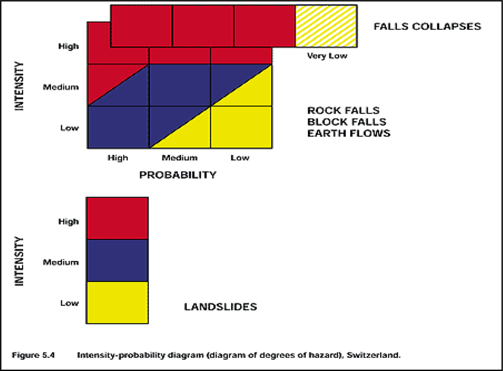
Hazard is defined as the occurrence of potentially damaging natural phenomena within a specific period of time in a given area [5,6]. Hazard maps are based on two major parameters: intensity and probability (or return period). According to the federal guidelines [4], three levels of intensity and probability are considered (high, medium and low) and the degree of hazard is classified in four colors, according to the matrix diagram shown in Figure 1: red for high hazard, blue for moderate hazard, yellow for low hazard, and white/yellow-hatched for residual hazard (i.e., high intensity but very unlikely) [7]. The estimation of the degree of hazard has a direct impact on the management and use of the territory. In the red zone people are at risk both inside and outside of buildings and construction in this zone is banned. Existing buildings can be maintained but no expansions are allowed. The blue zone indicates an area where people are at risk outside of buildings. Restrictive regulations must be followed and the construction type must be adapted to the present conditions. In the yellow zone there are no restrictive regulations and people living here only have to be notified of possible hazards.

For processes such as floods or earth flows, it is more straightforward to evaluate the event intensity and the associated return period. However, mass movements often correspond to gradual (landslide) or unique (falls) events. It is therefore often difficult to predict when a dormant landslide may be reactivated or to make an assessment about the return period of a collapse. The determination of the class of intensity of a landslide is thus based on the state of activity and, in particular, on the velocity under the assumption that landslides are more dangerous if moving fast. Estimating the rate of movement of a landslide is not easy and involves a wide margin of uncertainty. In a few cases, in fact, landslides are characterized by continuous movement over time and more frequently they go through periods of reactivation followed by phases of quiescence. Therefore, it is extremely important to determine the frequency of measurements and the window of time over which to extend them. According to the federal guidelines [4], a low intensity class can be assigned to landslides characterized by mean velocities below 2 cm/yr, representing a “permanent” activity. Medium intensity is defined by velocities reaching from 2 cm/yr up to 10 cm/yr. High intensity is a classification, where the velocity is higher than 10 cm/yr. Other criteria for the hazard assessment of landslides are the accelerations (changes of velocity), the shearing mechanisms, and the depth of the sliding surface [4]. Because landslides are usually non-recurring processes, the return period has only a relative connotation.

An indispensable prerequisite for hazard identification is extensive knowledge of past events on a regional scale, i.e., the compilation of a landslide inventory. Landslide mapping is also fundamental to evaluate hazard and aerial photography interpretation is an essential tool for the detection of landslides in vast alpine areas in support of field identification [8]. In order to correctly attribute a rate of displacement to a landslide, a suitable set of monitoring data, being at the surface (topographic measurements, GPS, extensometers, distometers) or in depth (inclinometer measurements in boreholes) is then needed. If these data are not available, the activity can be estimated by means of in-situ observations based on geomorphological evidences. However, the recognition of the rate of movement on large instabilities with slow and continuous movements (from millimeters to decimeters) is very difficult because the signs of activity can be easily masked by the development of shell debris and soils. The identification of differential movements of individual slope sectors is also difficult in the absence of buildings and infrastructures that show visible damages. Furthermore, slope movements become evident only after a minimal displacement has occurred and at that moment no monitoring data is usually available for any interpretation of the phenomenon. The lack of a displacement history for the landslide can hamper both the interpretation of the process and the forecast of future development. Information on landslide displacement from satellite SAR interferometry (InSAR [9,10]), in general, and from Persistent Scatterer Interferometry (PSI [11,12]), in particular, can be of great importance in these cases. InSAR and PSI displacement information can be integrated with previous landslide maps to reach a more complete and substantiated conclusion about the state of activity of slope instabilities [13–20].

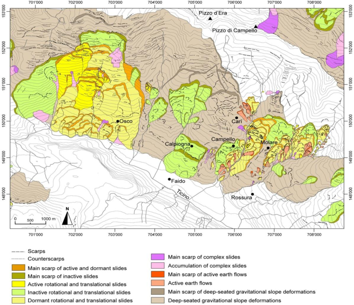
In this contribution we discuss our combined approach for landslide inventory based on aerial photographs and SAR interferometry for a region along the northern flank of the Leventina valley above Faido, which is affected by one of the largest deep-seated slope movements in Switzerland [21,22]. The deep-seated landslide is characterized by the presence, in the upper part of the slope, of a collection of counterscarps directed northeast with a movement of many tens of meters and a length up to 150 m. The lower half of the slope has a strongly convex profile resulting from numerous large rotational and translational slides, including that of Osco (Figure 2), whose activity has been known for a long time and of which we commonly refer to the deep-seated landslide.

2. Aerial Photography Interpretation

The interpretation of optical images is commonly applied in support of landslide’s inventories [8,15]. The analysis is based on stereoscopic aerial images of the same area taken from slightly different viewing positions and allowing therefore a three-dimensional reconstruction with an emphasis on heights. With this approach landslides can be easily recognized and, if the quality of the images is high enough, geomorphological features associated with the mass movements such as scarps, counterscarps, trenches, debris flows, rockfalls and debris fans can also be mapped. Based on aerial photography interpretation complemented by field surveys and historical records, landslide maps were produced for a number of catchments in the southern Swiss Alps [8]. The advantage of observing a wide portion of territory allows mapping of large landslides hardly recognizable through site surveys. On the other hand, the latter are indispensable in identifying failures of small dimensions hardly recognizable from aerial photographs.

The sketch map of the deep-seated landslide in Osco was carried out by analyzing 205 aerial photographs taken over the last 50 years, see

Table 1. Aerial photographs information.

Date	Fly Line	Photograph Number	Scale/Resolution
1961	9	from 8,896 to 8,900	1:19,900
1961	14	from 898 to 908	1:22,200
1961	15	from 8,931 to 8,933	1:25,700
1961	16	from 9,874 to 9,880	1:23,900
1961	33	from 9,161 to 9,172	1:20,800
1976	358	from 5,080 to 5,082	1:22,100
1976	368	from 5,112 to 5,114	1:22,100
1976	366	from 2,511 to 2,515	1:22,100
1977	15	from 5,141 to 5,143	1:20,000
1988	102	from 7 to 33	1:26,100
1988	103	from 1 to 31	1:26,100
1988	104	from 9 to 49	1:26,100
1988	105	from 1 to 31	1:26,100
1989	40	from 1,484 to 1,487	1:24,800
2001	148	from 3,140 to 3,149	1:27,500
2001	152	from 2,890 to 2,898	1:27,500
2001	156	from 2,843 to 2,852	1:27,500
2009	digital strips	939, 1,001, 1,023	50 cm
2011	digital strips	31, 51	50 cm

. All recognized phenomena, distinguished according to their type, were mapped and manually georeferenced in a GIS environment (Figure 3). The use of a high precision Digital Elevation Model (DEM), established by airborne laser scanning with an accuracy of 0.5 to 1.5 m, led to a georeferencing error lower than 5 m. The landslide map was then updated using the digital linear scanning images with photo-interpretation supported by the ArcGDS™ software. This method allows an important improvement in 3D cartography by collecting, editing and updating 3D features using a digital stereoscopic 3D interface. In addition to 2D (X-Y plane) data, ArcGDS captures altitude data (Z) by continuously connecting points in superimposed digital landscape scanning from different acquisition geometries. Using this digital method we obtain polygons with a georeferencing error of about 1 m. The landslide map was completed by assigning a database to each polygon with additional information such as area, volume, type of material involved, etc. The analysis of time series of aerial photographs made it possible to quantify the possible state of activity based on the more or less rapid changes of the morphology and on damages at local sites.

The recognized phenomena were distinguished such as slides, flows and deep-seated gravitational slope deformations. According to the classification introduced by [5,6], slides imply the movement in multiple blocks or in one single intact block by sliding along one or more surfaces. Typically, the distinction between rotational and translational landslides is introduced depending on the geometry of the sliding surface. The state of activity of the landslides is classified in active, inactive and dormant. Deep-seated saggings (or “Sackungen”) include large, deep, slow slope movements where deformations are distributed along various morphostructures or ductile and fragile structures without the presence of a single slipping surface [23–25]. Usually the size of these phenomena is comparable to that of a slope. Among the surface failures, earth flows relate to the mobilization of coarse material along with the production of rods, banks and grooves with V-profile. With the contribution of water flowing along streams and depending on the physical and mechanical characteristics of the materials involved, earth flows can travel great distances.

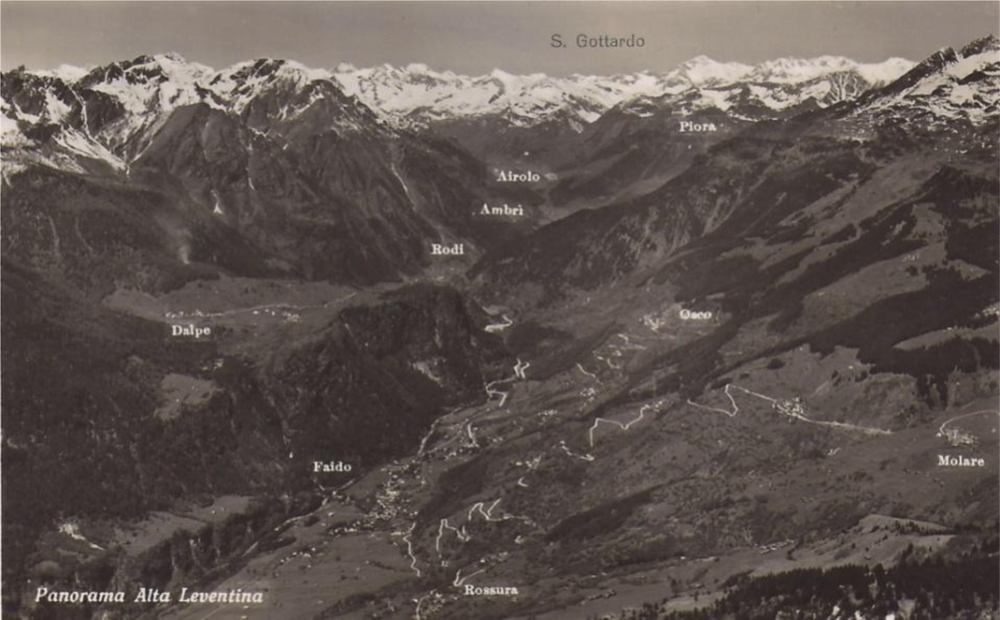
The deep-seated gravitational slope deformation of Osco covers an area of over 35 km² and ranges from an altitude of about 700 m a.s.l. at the bottom of the valley to more than 2,500 m a.s.l. at the highest peaks. In the area, granitic and metapelitic gneiss belonging to the Leventina and Lucomango nappes are present. As can be observed in Figure 2, the middle and lower parts of the slope are strongly vegetated, with meadows and forest, while rock outcrops are dominant at higher altitudes. Houses are mainly concentrated in villages. The main morphological evidence of the presence of a deep-seated landslide is the strongly convex profile in the lower half of the slope resulting from numerous large rotational and translational slides. A deep ravine delimits the western part of the “Sackung”, around the village of Osco, from the eastern part, where two active landslides to the east and west of the village of Molare are present. Evidence of the current state of activity of these landslides is indicated by the presence of numerous scarps which cut glacial deposits and show displacements of up to 50 m. In the eastern sector of the gravitational slope deformation between the villages of Campello and Rossura, ground motion—related to instability phenomena recognized by aerial photographs—are highlighted by a series of escarpments with a movement of up to 50 m affecting a thick layer of quaternary deposits. In 1987 a rotational slide occurred at the toe of the western sector and the Ticino River was partially dammed. Other damages were observed in the summer of 1993 and in November 2002, with a strong acceleration of the displacements corresponding to rain storm events.

3. Satellite SAR Interferometry

Repeat-pass Interferometric Synthetic Aperture Radar (InSAR) is a powerful technique for mapping land surface deformation from space at fine spatial resolution over large areas [9,10]. Displacement is derived from the measurement of the phase difference of the signals acquired by two satellite SAR acquisitions after compensation of the topographic effects with use of an external DEM of high quality (DHM25 © Swisstopo, 2009). Major advantages of this technique are the wide area coverage, the high sensitivity to surface displacement (centimeters to millimeters), and the availability since 1991 of a large archive of satellite acquisitions with repeat-cycles on the order of one month. Despite limitations due to vegetation cover, the special SAR viewing geometry, atmospheric artifacts, and snow cover, short-baseline interferograms are successfully applied in alpine areas for the mapping and monitoring of rock glaciers [26] and landslides [27]. Some of the limitations of the technique, due to the presence of vegetation or of very rapid displacements, can be partially overcome with the use of radar sensors with longer wavelengths [28,29].

The application of InSAR is limited by temporal and geometric decorrelation and inhomogeneities in the tropospheric path delay. In Persistent Scatterer Interferometry (PSI), differential SAR interferometry is applied only on selected pixels that exhibit a point-target scattering behavior and are persistent over an extended observation time period [11,12]. Through the use of many SAR scenes, even if separated by large baselines, errors resulting from atmospheric artifacts are reduced and a higher accuracy can be achieved. Over urban areas with numerous man-made structures or in regions where exposed rocks or single infrastructures (e.g., houses, power line masts) scattered outside cities and villages are visible, it is therefore possible to estimate the progressive deformation of the terrain at millimeter accuracy [30,31]. In mountainous regions the number of persistent scatterers is, however, limited by the sparse urbanization, the large forest cover, and areas of shadow and layover [32–37].

In our study, InSAR and PSI have been applied to stacks of ERS-1/2 SAR, ENVISAT ASAR and ALOS PALSAR images acquired between 1992 and 2010, excluding winter acquisitions with snow cover (

Table 2. Satellite SAR data considered in our study (A: ascending orbit; D: descending orbit).

Sensor	Track	Time Period	# Images
ERS-1/2 SAR	D 251	1992–2000	34
ENVISAT ASAR	D 251	2003–2010	29
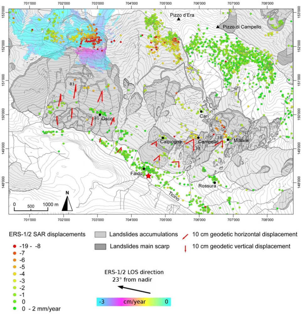
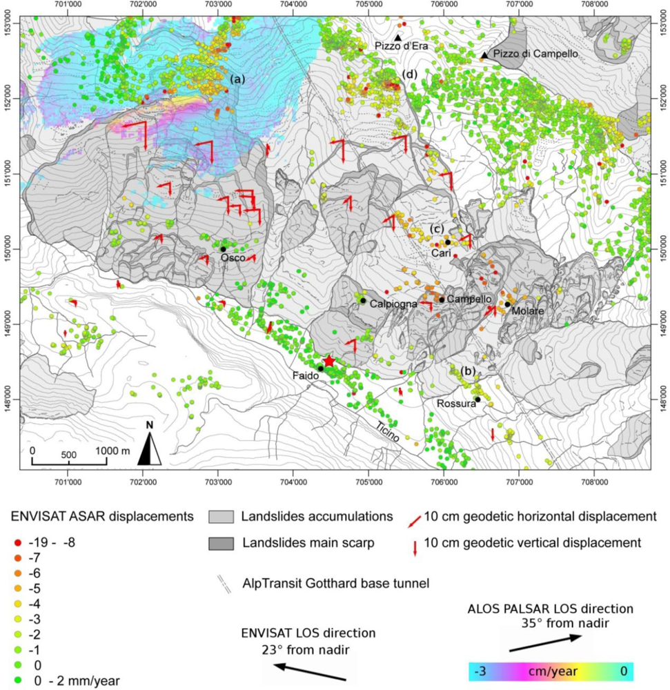
ALOS PALSAR	A 645	2007–2010	2

). Images from ascending and descending orbits were analyzed for a better spatial coverage. InSAR results consist of displacement maps for the acquisition time interval of the interferometric pair and were derived only for the upper western part of the landslide where movements are larger. PSI results consist of linear deformation rates and displacement histories. For every persistent scatterer within the study area it is thus possible to reconstruct the time-series of movement in the satellite Line-Of-Sight (LOS) direction (tilted by 23° with respect to the zenith) over a time period of almost 20 years. Reference points were selected individually for each of the sensors in areas estimated as stable. For the combined use of InSAR, PSI and aerial photography interpretation, the average displacement rates of coherent areas and point targets in the satellite LOS direction are plotted on the sketch maps with geomorphological features (Figures 4 and 5). Different color schemes are considered for InSAR and PSI. Negative values indicate an increase in the distance from target to satellite or, in general, a lowering of the surface.

In the eastern part of the slope, the ERS PSI average displacement rates (Figure 4) are in very good agreement with the landslides recognized by the aerial photo. In Campello and to the west of Molare relatively large displacement rates of 4 to 7 mm/yr are observed within particularly active sectors of the landslide. Because these values are along the satellite LOS direction, the actual motion is up to 2 cm/yr in this part of the landslide where the slope is oriented approximately southwest (∼210°) with an inclination of about 20° with respect to the horizontal direction. On the other hand, a slow motion of about 1 to 3 mm/yr is observed between the two landslides, including the village of Molare, and in Calpiogna. At the bottom of the valley no motion is observed. Also the eastern upper part of the slope does not show displacement, whereas toward the center, displacement values of 2 to 5 mm/yr are observed in the upper part for a large number of rocks. In the whole upper eastern sector of the slope, the rate of movements aligns well with the limit of the landslide identified by photo-interpretation.

In the western part of the slope, the ERS PSI displacement rates (Figure 4) are close to zero for the village of Osco. In accordance with the kinematics of a rotational landslide, the 3-dimensional displacement in this sector can be along a more horizontal direction so that the component along the satellite LOS is small. In the lower part of the landslide, the performance of PSI is severely limited by the vegetation cover. Above Osco, the ERS PSI displacement rates increase to values approaching 1 cm/yr and on top of that a clear signal with a magnitude on the order of 2 cm/yr is visible from a one year ERS interferogram between 1996 and 1997. This sector of the landslide corresponds to slipping phenomena with significant morphological evidence on the surface. Further up the PSI rates decrease to values lower than 1 cm/yr.

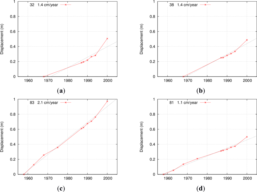
In the upper part of the western portion of the landslide the PSI displacement rates determined with ENVISAT (Figure 5) are generally lower than those measured with ERS. As can be observed in the time-series of Figure 6a, the rates of movement are non-linear, with larger values for the period 1998–2000. Shown along the ENVISAT PSI displacement rates in Figure 5 is an ALOS PALSAR interferogram acquired between 2007 and 2010 along the ascending orbit geometry. This ALOS interferogram is not from the same orbit geometry as the ERS and ENVISAT data and clearly shows the western border of the most active upper sector of the landslide, which is partly masked by layover in the descending orbit geometry. Here, rates of movements are larger than 3 cm/yr along the satellite LOS, two to three times more if projected along the direction of maximum slope.

Along the whole sector, from Rossura to Carì (Figure 6(b,c)), the rates of movements determined with ENVISAT are generally higher than those determined with ERS. This is possibly due to large scale consolidation, associated with pore-pressure reduction in the rock mass arising from drainage, associated with the drilling of the Alptransit tunnel at about 700–1,500 m depth beneath the topographical surface [38,39]. For many of the points in the upper eastern sector of the slope, the subsidence caused by the Alptransit tunnel drilling is masked by larger movements on the surface (Figure 6(d)). Here, a possible correlation of the displacements with 1993 and 2000 rain storm events has been detected.

4. Landslides Inventory

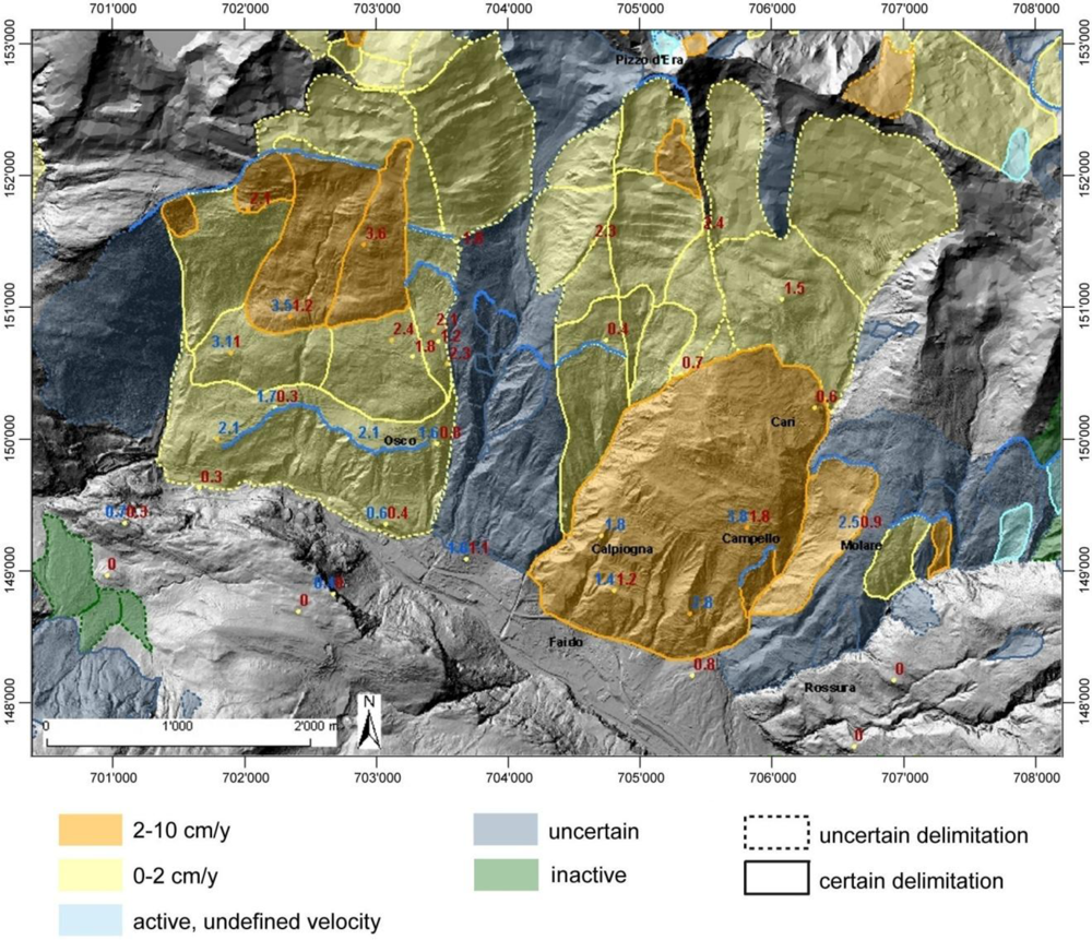
An inventory of landslides indicating the intensity classification has been compiled based on the sketch map from aerial photography and the surface displacement rates from InSAR and PSI (Figure 7). According to the model of the Swiss Federal Office for the Environment [40], five classes of intensity are distinguished: below 2 cm/yr, from 2 to 10 cm/yr, from 10 to 50 cm/yr, from 50 to 100 cm/yr, and above 100 cm/yr. For the deep-seated landslide in Osco, only the first two classes of intensity are present, i.e., maximum displacement rates are below 10 cm/yr. In the landslide inventory, two major sectors with higher rates of movements are indicated in orange (velocity > 2 cm/yr): one around Campello and one above Osco. Because the displacement rates calculated by PSI and InSAR are along the satellite line-of-sight direction, the real 3-dimensional displacements and velocities are two to three times higher than those plotted in Figures 4 and 5. The uppermost sector of the landslide above the village of Osco indicates very well how photo-interpretation is updated with motion information from satellite SAR interferometry. In the sketch map of Figure 3 we indicated an inactive slide for this sector, but ERS and ENVISAT displacement rates are up to 1 cm/yr here. In the inventory of Figure 7 we therefore indicate a polygon with a 0–2 cm/yr activity class. With respect to the sketch map from aerial photography the resolution of the inventory is coarser, because it has to cover the entire national territory at an approximate scale of 1:30,000. A distinction is made between certain and uncertain landslide delimitations based on the presence of well-defined geological structures or of a sufficient number of PSI points. In addition, a further class indicating uncertain presence of a landslide (e.g., weak indication in aerial photographs and absence of PSI points, inclusion in the register of event but without clear geological evidence) is introduced.

Available high resolution ground-motion geodetic data from classical trigonometric techniques (Figure 4) and GPS (Figure 5) are considered for validation. The geodetic measurements have been carried out since 1919 when the first 4th order trigonometric network for official measurement purposes was installed. During the subsequent measurements carried out in 1956 it was found that several of the trigonometric points had moved downstream significantly and in 1958 control measurements were performed in order to more precisely determine the velocity of the points subject to movement. Seven years later, in 1963, control measurements of the landslide were resumed by the road office with almost an annual repetition until 1975. After an interval of twelve years, geodetic control measurements were resumed by the cantonal geological office in 1987, continued thereafter biannually, and concluded in 2000. The difficulty in obtaining complete data sets over the entire observation period—as benchmarks were lost or moved—has led us to analyze only 15 points in Figure 4 within and around the landslide in Osco. For these control points, complete information about the planimetric and altimetric displacement vectors (3-dimensional), the average annual rates, and times-series of movement are available.

The analysis of the monitoring data available with classical trigonometric techniques reveals and highlights the heterogeneous movement of the landslide. Mean displacement rates of 1.4 cm/yr were measured for the two points around Campello in the eastern sector of deep-seated landslide; at lower altitudes rates were lower. Time-series of displacements over the last 40 years (Figure 8(a,b), No. 32 and 38) indicate an increase of velocity around 1994. In the middle of the western sector, average rates of movement are on the order of 2 cm/yr and the time-series (Figure 8(c), No. 83) indicates that the landslide state of activity has not been constant over the last 50 years. The lower part of the western sector has smaller rates of movement (Figure 8(d), No. 81) on the order of 1 cm/yr. An increase of the velocity around 1994 is also measured for both points: Numbers 81 and 83. Benchmarks in the upper part of the western landslide are indicated in Figure 5 but not in Figure 4, because they were not measured in 1992 and 2000. This shows the largest rates of movement with average velocities of around 5 cm/yr over the last century. This ratifies the large PSI and InSAR LOS rates of movement above Osco. The directions of the displacement vectors for the points on the western sector of the deep-seated landslide are in accordance with rotational kinematics: above Osco significant horizontal and vertical displacements are observed, while below Osco the trigonometric measurements indicate a nearly zero vertical component of the movement.

From 2000 onwards the network monitoring of the Osco landslide was conducted with GPS on a predominantly annual basis. The GPS monitoring network is not exactly composed of the same points of the geodetic network, because some new points were placed and inevitably some others disappeared. In the short time period from 2003 to 2010, the GPS measurements (Figure 5) confirmed the strongest movement of the western-upper sector and a decreasing trend towards lower locations. Also in the eastern sector, the largest rates of movement are found in the upper sector with values of more than 2 cm per year. The GPS points show a significant horizontal shift towards the west. A more thorough processing of the GPS data would have been required in order to determine rates of movement below a couple of cm/yr for an observation time period of about 10 years.

5. Conclusions

The identification of ground motion from InSAR and PSI complements the geomorphological information collected by photo-interpretation well. While the analysis of aerial photographs allows us to recognize numerous phenomena of instability and to define their limits, InSAR and PSI analyses allow us to characterize the intensity classification of landslides, using a deformation time-series extended over almost 20 years. In our analysis we frequently found conformity of the information from the two different techniques, such as the distinction of areas within or outside landslides in the upper part of the slope where displacements are, according to a rotational kinematics, almost vertical. Satellite radar interferometric analysis based on persistent scatterers has a higher added value where there are buildings—or other anthropogenic constructions—or areas with sparse vegetation and the presence of rocks. In vegetated areas (forest, meadows) application of this technique is more difficult, but depending on the radar sensor wavelength and geometry, some investigations are still possible using InSAR [28,29], particularly if complemented with information from other methods. The availability of geodetic monitoring data also allows validation of the PSI movement rates giving a higher level of confidence in the satellite-based technique.

The objective for our future work is to continue compilation of landslide inventories indicating intensity classification for all mountainous regions in Switzerland. This will represent a valuable instrument for a regional overview of slope instabilities. Such inventories from satellite SAR interferometry would be cartographic information to be used in combination with other geological data for the establishment of hazard maps officially created by the Cantons for their municipalities. For a more straightforward interpretation of motion rates observed by PSI and InSAR, investigations are ongoing regarding the direct transformation of the motion rates from the satellite line-of-sight direction into the direction of parallel slope. In this regard, particular attention has to be paid to the south and north facing slopes, which are not favorably illuminated by polar orbiting satellite SAR systems, to the resolution and quality of the DEM needed to calculate the direction of parallel slope, and to the kinematics of rotational slides, with almost vertical displacements in the upper part and almost horizontal displacements in the lower part. In future, the sustainability of SAR interferometric measurements will be guaranteed by the acquisitions of the very high resolution satellites TerraSARX, Cosmo-SkyMed and Radarsat-2 and by the planned new European satellite platform Sentinel-1.