Evaluation of CLM4 Solar Radiation Partitioning Scheme Using Remote Sensing and Site Level FPAR Datasets

Abstract

This paper examines a land surface solar radiation partitioning scheme, i.e., that of the Community Land Model version 4 (CLM4) with coupled carbon and nitrogen cycles. Taking advantage of a unique 30-year fraction of absorbed photosynthetically active radiation (FPAR) dataset, derived from the Global Inventory Modeling and Mapping Studies (GIMMS) normalized difference vegetation index (NDVI) data set, multiple other remote sensing datasets, and site level observations, we evaluated the CLM4 FPAR’s seasonal cycle, diurnal cycle, long-term trends, and spatial patterns. Our findings show that the model generally agrees with observations in the seasonal cycle, long-term trends, and spatial patterns, but does not reproduce the diurnal cycle. Discrepancies also exist in seasonality magnitudes, peak value months, and spatial heterogeneity. We identify the discrepancy in the diurnal cycle as, due to, the absence of dependence on sun angle in the model. Implementation of sun angle dependence in a one-dimensional (1-D) model is proposed. The need for better relating of vegetation to climate in the model, indicated by long-term trends, is also noted. Evaluation of the CLM4 land surface solar radiation partitioning scheme using remote sensing and site level FPAR datasets provides targets for future development in its representation of this naturally complicated process.

1. Introduction

Partitioning of incident solar radiation among various components at the land surface, especially from vegetation and underlying soil for vegetated regions, determines the energy absorbed by vegetation, evapotranspiration, partitioning between surface sensible and latent heat fluxes, and the energy and water exchange between the land surface and the atmosphere [1–10]. How solar radiation reaches underlying soil through between-crown gaps and within-crown gaps is an essential part of micrometeorological, climatological, biogeochemical, and hydrological modeling [11–15]. Various authors have explored numerical solutions to the partitioning problem, in both one-Dimensional (1-D) and three-Dimensional (3-D) geometries [13,16–19]. Though the complexity of the problem fully justifies the need for a 3-D model, 1-D models have been popular because of their ability to approximate it in a relatively simple form and to give reasonable results [16,17]. In the Community Land Model (version 4.0, CLM4), this process is formulated by a 1-D land surface solar radiation partitioning scheme: each sub-grid land cover type, plant functional type (PFT) patch, and bare soil, is a separate column for energy calculation [18,20]; a 1-D radiative transfer approximation is employed to simulate the radiative transfer process within canopy at PFT levels [18]. This study aims to address the performance of this modeling and how to improve it.

The fraction of absorbed photosynthetically active radiation (FPAR) is employed as the diagnostic parameter for the land surface solar radiation partitioning scheme. FPAR is defined to be the fraction of PAR absorbed by the canopy [21], and hence, should be decided mainly by the radiative transfer process within the canopy. However, it can also be affected by the solar radiation reflected by the ground since plants are not separated from their background in FPAR observations, either at site level or in remote sensing. Below-canopy PAR sensors at flux sites measure not only the PAR transmitted through the canopy, but also the PAR directly incident on the ground; digital information at each pixel in remote sensing represents the averaged spectral information from each surface type within the instantaneous field of view (IFOV). Therefore, FPAR is an appropriate parameter for this study.

In order to evaluate model performance, the dynamics of the fraction of absorbed photosynthetically active radiation (FPAR)’s seasonal cycle, diurnal cycle, long-term trends, and spatial patterns are used. The seasonal cycle of FPAR is essentially driven by leaf presence, growth, and foliage, so it can be interpreted as a manifestation of plant phenology. The diurnal FPAR cycle, however, is a more complicated process. It is orchestrated by the angular effect of direct solar radiation, fraction of direct radiation in total solar radiation, and vegetation coverage in the forest. The study of the diurnal cycle of FPAR is a novel utilization of flux tower observations. Diurnal cycle observations represent all aspects of canopy-sun-surrounding relations, while traditional studies, using site level observations, focus on the seasonal cycle and absolute value at the time when measurements are made, although series of these measurements may be collected over multiple days [22–26]. The long-term trends of FPAR could be impacted by two factors: plant phenology changes, such as leaf area index (LAI) and leaf out time, and plant distribution changes [27]. In addition to temporal dynamics, FPAR spatial patterns are also evaluated. Spatial patterns are decided mainly by plant types and geographical conditions [28]. As analyzed above, the accuracy of the solar radiation partitioning solutions depends, on not only the performance of the land surface solar radiation partitioning scheme, but also on the accuracy of input information on vegetation (e.g., LAI) and other conditions. Therefore, our evaluation needs to generally identify the reasons for discrepancies and focus on those problems related to the land surface solar radiation partitioning scheme.

Current remote sensing (RS) data, and the application of photosynthetically active radiation (PAR) sensors in flux tower networks, provide appropriate observations for evaluating the CLM4 land surface radiation partitioning scheme. Some satellite FPAR datasets have been produced based on various retrieval algorithms and radiative transfer assumptions [23,29,30]. Although they differ in absolute values, most remote sensing FPAR products are compatible with one another in seasonal cycle and spatial patterns [26,28,31]. The application of PAR sensors in a flux tower network enables evaluations of the FPAR diurnal cycle. PAR sensors provide highly accurate measurements of PAR, and have been put into service in many flux tower sites [22,32,33]. A systematic FPAR observation should consist of four parameters: incident PAR, reflected PAR, PAR transmitted through the canopy, and PAR reflected by the ground. Transmitted PAR should be measured by a group of PAR sensors because it is highly location-sensitive, while PAR reflected by the ground could be ignored if the soil reflectance is low. Such an integrated observing system exists at limited sites [32]. Hence, it is of great potential to use both satellite-based and site-level observations to investigate CLM4 performance regarding FPAR dynamics and spatial patterns.

We have three objectives: (1) to evaluate CLM4 performance in representing FPAR dynamics and spatial patterns; (2) to identify the agreements and disagreements between CLM4 FPAR and observations; and (3) to understand the reasons for those differences, and focus on the problems related to the land surface solar radiation partitioning scheme. In Section 2 we present the data and methods. The comparisons regarding FPAR dynamics and spatial patterns are shown in Section 3. Specific findings and implementations are discussed in Section 4, with conclusions drawn in Section 5.

2. Methodology

2.1. Model Description

As the diagnostic parameter for the model, FPAR’s accuracy reflects justifications of the land surface solar radiation scheme, but is not limited to this. Solar radiation (i.e., direct vs. diffuse radiation) and plant phenology (i.e., leaf area index (LAI)) are two factors also entering into the model’s calculation of FPAR. In this study, solar radiation (including direct and diffuse radiation), as prescribed in forcing data CRUNCEP [34], as estimated based on meteorological station observations (CRU dataset) and reanalysis product (NCEP dataset).

CLM4 represents the land surface as a hierarchy of subgrid types including glacier, lake, wetland, urban, and vegetated landunits. The vegetated part is further divided into patches of 16 PFTs and bare soil. Each subgrid land cover type is a separate column for energy and water calculation [18].

In each PFT patch, the vegetation fractional coverage is 100%. The two-stream module is employed to calculate the solar radiant fluxes that are reflected, transmitted, absorbed by the canopy, and that are absorbed by the underlying soil. Several assumptions are made, including that fluxes are isotropic in only two directions (upward and downward), the canopy is horizontally homogenous and elements inside the canopy (including leaves, stems, and trunks) are randomly distributed. The daily output of CLM4 sums up the fluxes from each PFT that includes bare soil and accounts for the fraction of vegetated area in the grid. In this study, CLM4 FPAR is defined as:

$$\mathit{FPAR}=\frac{{\sum }_{i=1}^{16}\hspace{0.17em}{w}_i{I}_{b,i}+{\sum }_{i=1}^{16}\hspace{0.17em}{w}_i{I}_{d,i}}{{\sum }_{i=0}^{16}\hspace{0.17em}{w}_i{S}_{b,i}^{\downarrow }+{\sum }_{i=0}^{16}\hspace{0.17em}{w}_i{S}_{d,i}^{\downarrow }}$$

(1)

where I_b,i (I_b,i) is the direct (diffuse) solar radiation absorbed by the canopy in the visible band for plant type i. $S_{b,i}^{\downarrow }\left(S_{d,i}^{\downarrow }\right)$ is the direct (diffuse) incident solar radiation at the land part of the grid in the visual band for plant type i[35], and w_i is the areal weighting of the plant functional type in the grid, ${\sum }_{i=0}^{16}{w}_i=1$, including bare soil (i = 0).

As for plant phenology, the plant phenology cycle in the CLM4 is fully-prognostic, resulting from coupling Carbon-Nitrogen (CN) model: the seasonal timing of new vegetation growth and litterfall responds to soil and air temperature, soil water availability, and day-length, in varying degrees depending on a specified phenology type for each PFT. LAI calculation is based mainly on the specific leaf area SLA (m² one-sided leaf area per gC) and the total canopy leaf carbon (C_L, gC ·m⁻² ground area) [36]. A linear relationship between SLA and canopy depth is assumed as:

$$\mathit{SLA}\left(X\right)={\mathit{SLA}}_0+mx$$

(2)

where SLA₀ is SLA at the top of the canopy, m is a linear coefficient, and x is a parameter describing the canopy depth as an overlying leaf area index. SLA₀ and m are both fixed for each PFT. Total canopy leaf carbon C_L can be found by integrating over the canopy:

$$C_L={\int }_0^L\frac{1}{\mathit{SLA}\left(x\right)}\hspace{0.17em}dx=\frac{\mathit{ln}\hspace{0.17em}\left[\left(mL+{\mathit{SLA}}_0\right)\right]-\mathit{ln}\hspace{0.17em}\left({\mathit{SLA}}_0\right)}{m}$$

(3)

Given C_L calculated from the CLM4, L can be solved as:

$$L=\frac{{\mathit{SLA}}_0\hspace{0.17em}\left[\mathit{exp}\hspace{0.17em}\left(m{C}_L\right)-1\right]}{m}$$

(4)

C_L is a dynamic carbon pool affected by gains from photosynthesis, and losses to litterfall and mortality, including from fire [37,38]. In addition to the dynamics of leaf carbon pool, feedbacks between carbon cycle and nitrogen cycle are also considered, which would also limit the rate of carbon accumulation in canopy leaf carbon [18].

2.2. Model Simulation

In this study the coupled CN version of CLM4 was driven by historical meteorological data CRUNCEP, land use and land cover, atmospheric CO₂ concentration, and anthropogenic nitrogen deposition. Beginning with the steady model state in 1901, CLM4 was run to 2009 with the previously mentioned historical forcings. Detailed information about the driver datasets and model settings can be referred to [39,40]. The half-degree monthly FPAR output during 2003–2005 was selected for direct comparison with all satellite observations due to the availability of remote sensing datasets. The period of 1982–2009 was selected for inter-annual change trend comparison between CLM4 FPAR and GIMMS FPAR3g.

2.3. Observation Data Description

2.3.1. Moderate Resolution Imaging Spectroradiometer (MODIS) Fraction of Absorbed Photosynthetically Active Radiation (FPAR)

The Moderate Resolution Imaging Spectroradiometer (MODIS) FPAR algorithm is based on 3-D radiative transfer theory. Inverse Look-Up-Tables (LUTs) are generated for six major biomes defined by MODIS; model configurations for each biome differ from each other by fractional coverage, structural characteristics including canopy height, leaf type, and soil color. Measured surface reflectances (atmospherically corrected bidirectional reflectances) at a maximum of seven spectral bands are used for the inversion [29]. The MODIS daily product is computed daily at 1 km resolution globally. The maximum FPAR value (across the eight days) is selected for the eight-day product [21]. Based on the eight-day product, Zhao [41] produced an improved product with cloud-contaminated pixels gap-filled.

2.3.2. Fraction of Photosynthetically Active Radiation (FPAR) 3g/Leaf Area Index (LAI) 3g Derived from Global Inventory Modeling and Mapping Studies (GIMMS)

GIMMS FPAR3g/LAI3g is computed based on improved versions of MODIS FPAR/LAI [42,43] and GIMMS NDVI3g generated from the Advanced Very High Resolution Radiometeters (AVHRR) using an artificial neural network. GIMMS NDVI3g and its long-term (June 1981–2011) global coverage at frequent intervals provide a unique opportunity to explore vegetation long-term dynamics [44]. It is therefore used as the sole dataset for long-term trend evaluation. However, the AVHRR data lacks correction for aerosol scattering and water vapor absorption [45], resulting in possible atmospheric artifacts in the GIMMS data sets.

2.3.3. Joint Research Center (JRC) FPAR

The Joint Research Center (JRC) generic FPAR algorithm has been used to develop FPAR products for both Sea-viewing Wide Field-of-view Sensor (SeaWiFS) and Medium Resolution Imaging Spectrometer (MERIS) [30,46]. It is not biome-specific, but defines FPAR as “green” instantaneous FPAR under direct illumination. Its input data are top of atmosphere (TOA) bidirectional reflectance factors (BRFs) in blue, red, and near-infrared bands. Blue band is used to remove the atmospheric effects [47]. For the monthly composite, median values which are the closest to the temporal average estimated over the compositing period are selected to generate the statistics [48].

2.3.4. Site-Level FPAR

We use data from the Bartlett Experimental Forest flux tower site (44.06°N, 71.29°W, and 272 m elevation) in north central New Hampshire, USA. This measured data is available from the AmeriFlux Web page [49]. Half hour-averaged measurements from 1 January 2005 to 30 December 2006 were used in this study. The vegetation is primarily deciduous forest [28]. The flux tower is 25 m in height and set in a relatively flat area. Quantum sensors are placed above and below the vegetation canopy. Above-canopy sensors are located at the top of the tower, sensors facing upward measure the incident photosynthetic photon flux density (Q_incident) while sensors facing downward measure the photosynthetic photon flux density reflected from the canopy (Q_reflected). Six below-canopy sensors are placed in a circle (radius = 15 m) centered at the base of the tower [32]. They face upward and thereby measure the photon flux density transmitted through the canopies or gaps (Q_transmitted). Site-level FPAR is calculated by:

$$\mathit{FPAR}=\frac{Q_{\mathit{incident}}-Q_{\mathit{reflected}}-Q_{\mathit{transmitted}}}{Q_{\mathit{incident}}}$$

(5)

Multiple sites for various plant types are desired to rigorously evaluate the model’s performance. However, due to the data availability, Bartlett Experimental Forest flux tower site was initially selected in this study to qualitatively diagnose model’s performance in deciduous forest.

2.4. Assessment of Consistency between Model and Observation Data Sets

Several analyses were performed over various temporal and geographical extents. Diurnal cycle was performed over the Bartlett Experimental Forest flux tower site from 2005 to 2006, seasonal cycle and spatial patterns were performed globally from 2003 to 2005, and long-term trends were conducted globally over the 28-year period of 1982–2009.

Prior to the analysis, data were resampled by averaging at 0.5° resolution if needed, grids defined as non-vegetated in MODIS, and dominant vegetation distribution was masked in all datasets. To assess the consistency between the model simulated FPAR and observations, several sets of analyses were performed as follows:

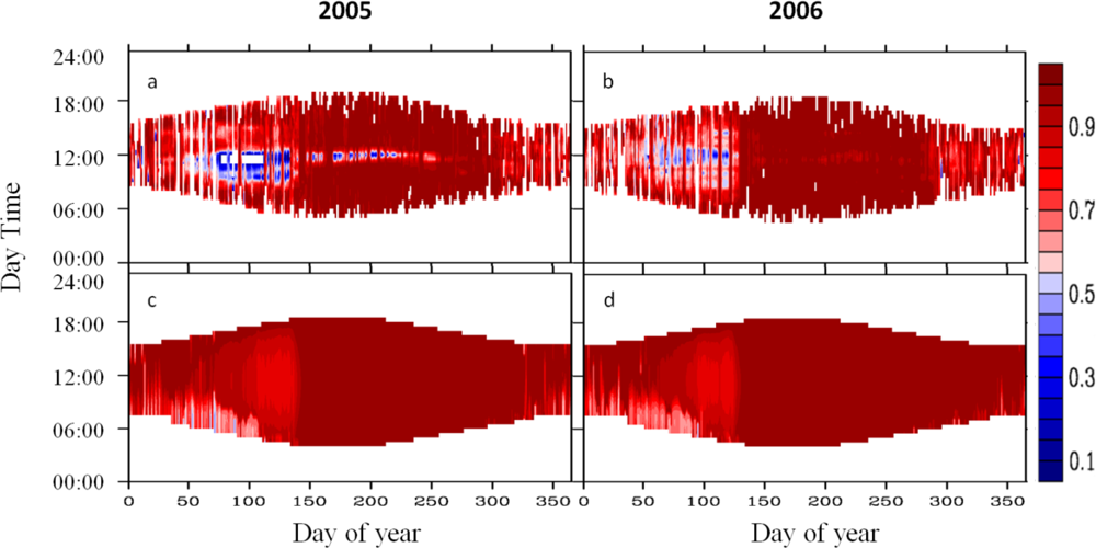
2.4.1. Diurnal Cycle

Prior to the analysis, observation on rainy and cloudy days were eliminated, because clouds and aerosols control the ratio of diffuse to total incident solar radiation [50], and diffuse radiation is less sensitive to the solar angle. Rain and cloud are decided by precipitation measurement and diffuse solar radiation (if diffuse PAR > 500 μmol/(m²·s), respectively. To better present the diurnal cycle, half-hourly FPAR data were normalized at a daily level by:

$$\mathit{FPA}{R}_{n\left(i,j\right)}=\frac{{\mathit{FPAR}}_{a\left(i,j\right)}}{{\mathit{FPAR}}_{\mathit{max}\left(i\right)}}$$

(6)

where FPAR_n(i,j) is normalized FPAR on day i, at time j, FPAR_a(i,j) is FPAR on day i, at time j, FPAR_max(i) is maximum FPAR on day i.

2.4.2. Seasonal Cycle

FPAR seasonal cycle comparisons are made at two spatial scales: global and aggregated by dominant MODIS vegetation types. The MODIS FPAR algorithm uses the MODIS land cover product with the International Geosphere Biosphere Program (IGBP) classes [44,51]. The JRC generic FPAR algorithm does not consider land cover type [45,46]. The CLM4 has a subgrid system representing vegetation as patches of PFTs that are derived from various datasets including MODIS Vegetation Continuous Fields data, AVHRR Continuous Fields Tree Cover Project data, MODIS global land cover mapping, Ramankutty and Foley global cropping, and Willmott and Matsuura climate data set [52]. As MODIS and CLM4 use different vegetation classification systems, the dominant vegetation distribution from MODIS is employed for the comparison of this paper. We define the dominant biome type in each half-degree grid as the land cover for the grid [53]. Prior to the analysis, monthly FPAR were averaged for each grid over 2003 to 2005. Monthly FPAR data at global and biome level were calculated by:

$${\mathit{FPAR}}_{a\left(m,b\right)}=\frac{{\sum }_{i,j}\hspace{0.17em}{\mathit{FPAR}}_{a\left(m,i,j\right)}\times {\mathit{Area}}_{i,j}\times {\mathit{frac}}_{i,j,b}}{{\sum }_{i,j}\hspace{0.17em}{\mathit{Area}}_{i,j}\times {\mathit{frac}}_{i,j,b}}$$

(7)

where FPAR_a(m,b) is FPAR in month m for biome b (or for the global, if b = 0), FPAR_a(m,i,j) is FPAR at computational grid (i, j) in month m, Area_i,j is the area for the grid (i,j), frac_i,j,b is the fraction of land unit at computational grid (i, j). Grids that are not dominated by the target biome were defined as frac_i,j,b = 0. Correlation coefficients (i.e., correlation and p-value) are calculated based on FPAR_a(m,b). Monthly FPAR anomalies at global or biome level were calculated by:

$${\mathit{FPAR}}_{\mathit{ano}\left(m,b\right)}={\mathit{FPAR}}_{a\left(m,b\right)}-{\mathit{FPAR}}_{\mathit{mean}\left(b\right)}$$

(8)

where FPAR_ano(m,b) is FPAR anomaly in month m for biome b (or for the global, if b = 0), FPAR_mean(i) is averaged FPAR over the whole time period.

2.4.3. Long-Term Trends

Long-term trends are calculated based on GIMMS FPAR3g and CLM4 FPAR from 1982 to 2009 by linear regression. For each 0.5°pixel, the slope and significance level (indicated by p-level) were calculated from time series comprised of 28 annual mean values (one value for each year from 1982 to 2009). Trends in LAI are also calculated in order to diagnose source discrepancies.,

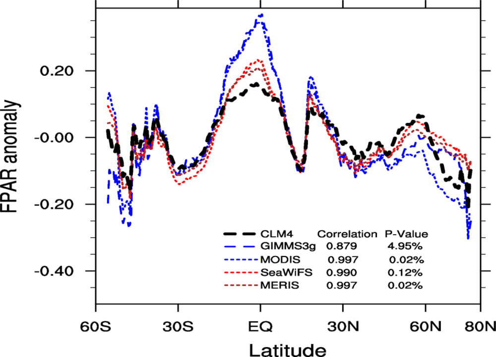
2.4.4. Zonal Patterns

Similar to monthly FPAR, zonal FPAR were also calculated by the grid area and land unit fraction:

$${\mathit{FPAR}}_{a\left(i\right)}=\frac{{\sum }_j\hspace{0.17em}{\mathit{FPAR}}_{a\left(ij\right)}\times {\mathit{Area}}_{i,j}\times {\mathit{frac}}_{i,j}}{{\sum }_j\hspace{0.17em}{\mathit{Area}}_{i,j}\times {\mathit{frac}}_{i,j}}$$

(9)

where FPAR_a(i) is the averaged FPAR for latitude band i. FPAR_a(i,j) is FPAR at computational grid (i, j), Area_i,j is the area for the grid (i, j), frac_i,j is the fraction of land unit at computational grid (i, j). Zonal FPAR anomalies at global or biome level were calculated by:

$${\mathit{FPAR}}_{\mathit{ano}\left(i\right)}={\mathit{FPAR}}_{a\left(i\right)}-{\mathit{FPAR}}_{\mathit{mean}\left(i\right)}$$

(10)

where FPAR_ano(i) is FPAR anomaly for computational latitude band i, FPAR_mean(lat) is the mean value for the averaged FPAR of all latitude bands.

2.5. The Angular Effect in Fraction of Absorbed Photosynthetically Active Radiation (FPAR) under Direct Solar Radiation

To illustrate the angular effect in FPAR with direct solar radiation, we regard tree crowns as spheroids-on-sticks (Figure 1). K_g and K_c are the sunlit background portion and the sunlit canopy portion, respectively. They correspond to the areal fraction of ground and canopy under direct solar radiation.

According to the Boolean Scene Model introduced in [54], in a sparse random distribution of the spheroids, the sunlit background portion is:

$$K_g=e^{-\lambda A_v\left(\theta \right)}$$

(11)

where $\lambda =\frac{n}{A}$ is the number of canopies in a unit of surface area, and A_v(θ) is the average areal projection of the canopy onto the background at the zenith angle θ. From this expression for K_g, the proportion of sunlit canopy portion can be immediately obtained, as both sum to 1.

$$K_c=1-e^{-\lambda A_v\left(\theta \right)}$$

(12)

For a single canopy area at vertical angle, A_v(θ) = πrb, where r and b are the horizontal and vertical radius of the spheroid, respectively. For the off-vertical angle, A_v(θ) = πrb/cosθ. Thus, we have:

$$K_c=1-e^{-\lambda \pi rb/\mathit{cos}\theta }$$

(13)

Therefore, as the solar zenith angle decrease, the canopy intercepts less direct solar radiation, resulting in the angular effects in FPAR under direct solar radiation. It is important to note that such an effect is restricted to sparse vegetation. For a fully-vegetated area under direct solar radiation, the angular effect is negligible, because the bare soil is thoroughly covered by the vegetation and thus receives little solar radiation, regardless of how the solar zenith angle changes.

3. Results

3.1. Diurnal Cycle

As illustrated earlier regarding angular effect, a canopy attenuates a larger fraction of the incident solar radiation in the morning and a much smaller share at noon. Therefore FPAR is expected to have a valley around noon.

Figure 2 shows the normalized FPAR for each day in 2005 and 2006 from both observations and model. From the site-observed FPAR figures (Figure 2(a,b)), we can see the minimum value occurring around noon in the early-growing months (March, April and May, MAM), which is only around 30% of the maximum FPAR. It verifies the angular effects of FPAR that we illustrated earlier. Minimum value is also shown around noon in MAM in the model simulated FPAR (Figure 2(c,d)), but is around 80% of the maximum FPAR. Figure 3 shows the monthly gross primary production (GPP) estimation from site observations [55]. It shows that the vegetation at the site starts photosynthetic activities in March and peaks in July. This peak possibly indicates the fully-grown canopy (i.e., high LAI values). By comparing Figures 2 and 3, we notice that the diurnal cycle is more significant before the GPP peak month (usually June for this site). One possible reason is that the between-crown gaps have been filled in by growth of leaves (high LAI) when GPP peaks. This assertion might explain the inter-annual differences between 2005 and 2006. Diurnal cycles exist with a clear valley pattern around noon after the GPP peak (July) in 2005, but not in 2006. Correspondingly, the GPP peak in 2005 is around 0.5 μmol/(m²·s) lower than that in 2006 (Figure 3). Since GPP is a good indicator for LAI, the lower GPP in 2005 suggests a lower LAI, and thus between-crown gaps cannot be filled by lower LAI canopies.

The CLM4 FPAR diurnal cycle is shown in Figure 2(c,d). The model shows a much weaker diurnal cycle in MAM without a valley around noon. This suggests that CLM4 did not adequately simulate the solar angular effect, although some sun angle dependence may have been included in the model. As for the angular effect we discussed, the solar zenith angle change from 90° in the morning to a minimum angle at noon should result in a large change in FPAR. In sum, we have three findings: (1) the site level FPAR diurnal cycle shows patterns that we expected when canopies are not fully grown; (2) the CLM4 land surface solar radiation partitioning scheme does not adequately reproduce the diurnal cycle in FPAR at these times; and (3) though the fractional cover of the canopies do not change, leaf growth influences between-crown gaps and as such the angular effect in FPAR.

3.2. Seasonal Cycle

In an additional global level, we selected ten major biomes among the seventeen vegetation types defined by the IGBP to conduct the comparison. Figure 4 shows CLM4 generally captured the seasonal variations displayed by satellite-based FPAR. CLM4-FPAR and remote sensing FPAR have good correlation over the global and most biomes (

Table 1. Correlation coefficient γ with P-value between CLM4-FPAR and satellite-observed FPAR annual cycle from 2003 to 2005.

	GIMMS3g		MODIS		SeaWiFS		MERIS
	γ	p-value	γ	p-value	γ	p-value	γ	p-value
Global	0.953	3.36E-04	0.942	3.34E-04	0.894	8.65E-06	0.873	9.25E-05
Evergreen Needle Leaf Forest	0.86	0.66	0.86	3.28E-04	0.934	0.96	0.893	0.44
Evergreen Broad Leaf Forest	0.14	2.35E-05	−0.860	4.10E-06	−0.016	4.11E-07	0.246	5.25E-06
Deciduous Needle Leaf Forest	0.919	1.90E-05	0.944	1.91E-04	0.965	1.57E-05	0.941	6.61E-06
Deciduous Broad Leaf Forest	0.923	1.78E-05	0.875	2.92E-05	0.926	2.09E-05	0.938	4.34E-05
Mixed Forest	0.924	1.92E-07	0.916	4.78E-07	0.921	1.35E-08	0.908	1.01E-08
Open Shrublands	0.97	1.96E-02	0.964	2.56E-05	0.982	1.22E-04	0.983	2.55E-04
Woody Savannas	0.66	0.94	0.918	0.90	0.887	0.28	0.868	0.11
Savannas	0.024	1.80E-06	0.042	1.51E-06	0.341	1.35E-05	0.487	1.58E-05
Grassland	0.952	2.07E-06	0.954	1.13E-05	0.928	8.99E-05	0.926	2.43E-04
Croplands	0.95	3 1.70E-06	0.942	4.59E-06	0.894	8.83E-05	0.873	2.12E-04

). However, CLM4 FPAR generally has smaller seasonality and a shift during peak months. For savannas, CLM4 fails to capture the peak and trough months, and seasonality in CLM4 is less pronounced than in the satellite observations (Figure 4(i)). Savannas-dominated grids exist in the Sahel region, Southeast Africa and in the western part of South America. These areas are characterized by seasonal water availability, with most of their rainfall confined to one season. Correspondingly, we can see strong seasonality from the satellite observations (Figure 4(i)). However, this discrepancy in seasonality is possibly related to the model parameterization of LAI estimation rather than to the land surface solar radiation partitioning scheme. It should be noted that the model and remote sensing agree well in that the evergreen broadleaf forest retains a rather stable FPAR all year round, though the correlation between them is rather low due to discrepancies in anomalies. However, their anomalies vary through a range smaller than 0.05 (Figure 3(c)), which is consistent with the relatively stable phenology in tropical rainforest.

In order to identify the reasons for the discrepancies in FPAR seasonality, we compared the seasonality of CLM4 LAI and GIMMS LAI3g to various estimates of FPAR (Figure 5). CLM4 LAI lacks seasonal variations in comparison with GIMMS LAI3g at the global level (Figure 5(a)), which can explain why CLM4 FPAR has fewer seasonal variations. For savannas, significant disagreements in FPAR, between model and observations, are also shown to have similar discrepancies in LAI (Figure 5(b)). As asserted earlier, the FPAR seasonality could be considered as a manifestation of plant phenology. The comparisons between LAI and FPAR, from the model and observations, verify this assertion and, hence, suggest that the discrepancies in seasonality between CLM4 FPAR and observations are due to problems in the calculation of LAI.

3.3. Long-Term Trends

Figure 6 displays the statistics of the long-term analysis. The color represents the slope of linear regression fit for the annual mean FPAR and the black dots are grids exceeding 90% significance. GIMMS FPAR3g (Figure 6) shows that Western Europe, Eastern America, the Sahel region, part of Eurasia, and the northern high latitudes are the areas with significant increasing trend in FPAR and LAI. Among these areas, changes in Western Europe are due to the afforestation of former arable land [56], an anthropogenic factor that is already included in the current CLM4. The rest of the areas are all transitional ecoregions: the Sahel region is a transition zone of semi-arid grasslands, savannas, steppes, and thorn shrublands lying between the Sahara desert and the Sudanian Savannas [57]; Eastern America and part of Eurasia are transitional zones of coniferous and broadleaf trees; the northern high latitudes are mainly the Arctic tundra ecosystem which is also ecologically transitional due to climate change [58]. As the satellite observations shows, these areas are highly sensitive to global climate change and thus have significant long-term trends.

The CLM4 simulations are in broad agreements with the increasing trends illustrated by GIMMS3g datasets (Figure 6). However, the model has fewer grid cells exceeding the statistical significance level of 90% (Figure 6). Since long-trends are primarily driven by changes in forcing factors (e.g., CO₂ concentration, precipitation, and temperature), these discrepancies suggest that the CLM4 needs to improve its correlation between climate and vegetation. Annual changes of vegetation growth possibly caused by other factors such as nitrogen deposition and land use and land cover change are beyond the scope of this paper and are detailed in [40]. Although our study does not examine land cover change, extensive FPAR increase in the northern high latitudes suggests dynamic vegetation change (Figure 6(b)). As several studies asserted, shrub expansion exists in Northern Alaska, Siberia, and the Pan-Arctic [59–61]. It would thus be necessary to employ a dynamic vegetation model (e.g., Dynamic Global Vegetation Model, DGVM) to reproduce expansions of certain plant types. In sum, we have two findings in regards to the CLM4: (1) CLM4 does capture the long trends in FPAR at the global level, but has much smaller significance levels due to its excess variability in its annual values; (2) discrepancies in the northern high latitudes further suggest that CLM-DGVM is required to fully evaluate model’s performance for long-term trends.

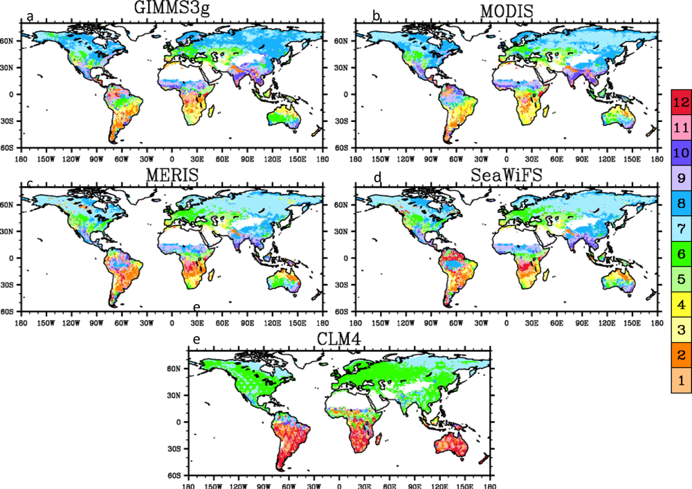
3.4. Spatial Patterns

The zonal anomalies of FPAR from 2003 to 2005 are displayed in Figure 7 and the correlation coefficients between CLM4 and RS FPAR are also calculated. CLM4 FPAR has a very similar pattern to that of remote sensing observations. Statistics show that they are highly correlated (0.879 for GIMMS3g, 0.997 for MODIS and MERIS, and 0.990 for SeaWiFS), and these correlations are all significant (p < 5%). They all have peaks around the equator and 25°N, and troughs around 30°S and 15°N. The difference between FPAR at the equator and the 25°N in CLM4 simulation is around 0.071, which is much smaller than that in GIMMS3g (0.203) and MODIS (0.162), and close to that in SeaWiFS (0.113) and MERIS (0.079). Figure 8(g) shows the month of maximum FPAR simulated by the CLM4. Compared with remote sensing observations (Figure 8(a–d)), the CLM4 does well in capturing the main characteristics of the FPAR peaking in June-July-August (JJA) in the northern hemisphere and in December-January-February-March (DJFM) in the southern hemisphere. However, the peak months in the CLM4 are generally one or two months earlier. The CLM4 simulations also have much less spatial heterogeneity in the month of maximum FPAR. Take north hemisphere for instance, satellite observations show FPAR peaks in June for Southern north America and west Europe, in July and August for northern north America and most Eurasia. The CLM4, however, estimates FPAR in most north hemisphere peaks in June with small high latitude area peaks in July.

In the Amazon, CLM4 FPAR and satellite-based FPAR have an interesting discrepancy. Satellite-observed FPAR for evergreen broadleaf forest shows weak seasonality (Figure 4(c)), but the spatial distribution of month with the maximum FPAR value has an unexpected pattern. Divided by the equator, FPAR in the northern part of the Amazon peaks around November, December, and January, while in the southern part it peaks around June, July, August, and September (Figure 9(a,b,d)). The probability density function of month with maximum FPAR value (Figure 9(f,g)) verifies that such differences exist among satellite-based observations. However, CLM4 FPAR has an opposite temporal-spatial distribution as we can see from Figure 8(g). The probability density function of month with maximum FPAR value (Figure 9(f,g)) also verifies such differences between the CLM4 FPAR and satellite-based FPAR.

4. Discussion

4.1. Problems with the Diurnal Cycle in the CLM4

Comparison of site level observations and model simulations shows CLM4’s FPAR has a slight diurnal cycle (FPAR at noon is around 80% of the maximum) but at a much smaller magnitude than site level observation (FPAR at noon is around 30% of the maximum). Sun angle could influence radiation transfer process through both between-crown gap probability and within-crown gap probability [19]. In order to identify the reasons for the insignificant angular effect in the CLM4, we used the 2-stream module from the CLM4 and conducted a sensitivity test in a two-element model that is simplified from the current CLM4 land surface scheme. In the two-element model, a grid is set consisting of two patches: one is vegetated with 100% canopy coverage, its coverage is set to be fc; and the other is bare soil with a fraction of (1 − fc). Related parameters are set as follows: (1) leaves and stems are set as blackbodies with reflectance and transmittance of 0; (2) ground albedo is 0.2 for both visual and infrared bands, and for both direct and diffuse radiation; and (3) only direct solar radiation is considered. We calculate the fraction of canopy absorbed radiation in incident solar radiation for the whole grid under different fc and LAI conditions. A 3-D model is used for comparison. It is a new framework based on the single bush model [13,62]. A one-layer canopy model is constructed that considers shadows, inter-canopy interactions, and the consequences of low sun (elevation) angles. It is used to build a three-layer canopy that considers ground shadow, within-crown gaps, between-crown gaps, and inter-canopy interactions, and thus is regarded as a benchmark [13,62].

Experimental results (Figure 10) show the fraction of radiation absorbed by canopy would change according to the solar zenith angle when LAI is low (i.e., 0.5). This verifies that the minor diurnal cycle in the current CLM4 simulation is attributed to the 2-stream solution, taking into account the angular effect inside the canopy layer. Such an angular effect in the canopy radiative transfer process only contributes to only a small portion of the overall angular effect (as illustrated by the 3D scattering model in Figure 10) Therefore, the problem with the diurnal cycle in the CLM4 is not the radiative transfer process within the canopy but rather the radiative transfer process outside of the canopy.

Next we examine the current CLM4 patch framework. Bare soil and plants are separately allocated into different patches. For the patch with a plant type, the canopy fraction is set to be 100%. According to this assumption, the plants become “shadowless”; only the soil under the canopy might be blocked from solar radiation by the canopy, but the soil between canopies can always receive solar radiation without any canopy blocking as allocated in a separate patch. As a result of this “shadowless” canopy assumption, the bare soil is 100% exposed to solar radiation, and such a full-exposure in bare soil is the reason for the absences of an angular effect in the current CLM4. Therefore, we need to introduce several parameters to present such an angular effect.

We propose a possible solution for this problem in the current CLM4 land surface scheme and illustrate it in a two-element model. The solution is based on the boundary condition inferred from the Boolean Scene Model: (1) vegetation has 100% coverage over the grid land when the solar zenith angle is 90°; and (2) a coverage of (fc) when the solar zenith angle is 0°, in the view of the sun.

By the view of direct solar radiation, the fraction of vegetation in the grid (fv) should be a function of fc and the solar zenith angle (θ):

$$fv=e^{\mathit{ln}\hspace{0.17em}\left(fc\right)\times \mu }$$

(14)

where μ= cosθ. The fraction of bare soil in the sun’s view should be 1 − e^ln(fc)×μ, and the fraction of sunlit bare soil in total bare soil (fss) is:

$$fss=\frac{1-e^{\mathit{ln}\hspace{0.17em}\left(fc\right)\times \mu }}{1-fc}$$

(15)

By this function, the bare soil would receive no direct solar radiation when μ = 0 and would be 100% sunlit by direct solar radiation when μ = 1.

This solution is a simplified approximation for the angular effect. Figure 11 shows it has good approximation when vegetation coverage is high or when LAI is high, compared to the 2D scattering model. Larger discrepancies exist when both vegetation coverage and LAI are low. The relationship between vegetation coverage and LAI is not considered here but has been suggested by site level observations. As analyzed earlier, the inter-annual comparison of site level FPAR suggests that vegetation coverage (fc) changes according to LAI. Hence, LAI-fc relation should be taken into account to implement mathematical representation of an angular effect in the current CLM4 land surface solar radiation partitioning scheme.

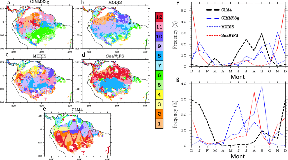
4.2. Spatial Patterns of Month with Maximum Fraction of Absorbed Photosynthetically Active Radiation (FPAR) in the Amazon

As previously illustrated, both the northern and southern parts of the Amazon have different peak FPAR months opposite to their located hemispheres. The angular effect in FPAR is suspected to be one reason for this phenomenon. One major difference between the two regions is the solar zenith angle. According to the angular effect, FPAR would decrease as the solar zenith angle increases and thus, the FPAR would not peak in local summer months. CLM4’s opposite estimations then can be well explained because model does not consider the angular effect in FPAR. However, one weakness in this reasoning is that the angular effect is more significant for sparse vegetation, but the Amazon rainforest has dense vegetation, and another weakness is that tropical latitudes have relatively muted seasonal variation in solar angle.

In addition to the angular effect, two other possibilities (i.e., cloud contamination and plant phenology) are also suspected to contribute to this phenomenon.

Cloud contamination is suspected to be a reason because remote sensing of the Amazon at visible bands has been complicated due to the presence of persistent cloud and aerosols during the rainy season. Remote sensing has made much effort in minimizing the cloud influence by: (1) recording cloud information into the raw data and pixels of good quality are selected for product generation; and (2) cloud-removal procedures to MODIS’s surface reflectance products. However, these procedures still cannot totally avoid the potential systematical bias in FPAR. As cloud contamination lowers the FPAR value, we would expect peak months to have the least precipitation in the region. For the southern part of the Amazon, remote sensing observations (Figure 9(g)) shows FPAR peaks in June, July, August, and September which are the months with much less rainfall (Figure 12). For the northern region, satellite data (Figure 9(f)) displays that FPAR peaks in November, December, and January by different satellite observations, which are months with less rainfall in the region (Figure 12). Therefore, cloud contamination might be the reason for spatial patterns in satellite observations.

The other possibility is associated with the seasonal cycle of plant phenology. Site level measurements show the photosynthesis of plants in the Amazon increases during dry seasons [63,64]. The dry season has less rain but offers more solar radiation, plus water is not limited in this region, so plants have better conditions for photosynthetic activities resulting in a higher FPAR value for light-rich, dryer days. The model might lack of such a complicated mechanism due to its deficiencies in calculations of soil moisture or root distribution [65,66].

4.3. Absolute Value

The absolute value of CLM4 FPAR is not evaluated due to disagreements among observational datasets. Inter-comparison among satellite-based FPAR products (Figure 13) shows discrepancies among them, and such disagreements have been noted in many remote sensing evaluation papers [28,31,67]. There are many factors contributing to these discrepancies. First, the satellite passing time is different for each satellite. We have illustrated how the angular effect in direct solar radiation would lead to an FPAR difference. Second, their statistical methods differ. MODIS selects the maximum FPAR (across the eight days) for the eight-day product [21] while SeaWiFS and MERIS use the median value in generating their products [48]. Last, radiative assumptions are different for different retrieval algorithms, though their influences require more study. Therefore, CLM4-FPAR’s absolute value is not be evaluated in this study. The difference in the absolute value is removed by subtracting the temporal averaged value for evaluation on diurnal and seasonal cycles and spatial patterns. The absolute value is used to calculate linear regression in long-term trend analysis, but does not affect the slope which is the key statistical parameter we analyzed.

4.4. Comparison with Previous Study

Several studies have compared satellite observations and CLM simulations. Tian et al.[35] compared seasonal and spatial variations of FPAR from MODIS and CLM2.0 from 2000 to 2002, and attribute FPAR mainly decided by LAI. Mao et al. (2009) compared MODIS GPP with CLM4 GPP regarding magnitude, phase, annual cycle, and inter-annual changes. Our study recognizes the role of LAI in FPAR simulation and targets the solar radiation scheme, so we identify reasons for discrepancies first and then focus on those associated with the target. General agreements in FPAR’s seasonal cycle, long-term trends, and spatial patterns are consistent with conclusions in previous GPP evaluations [53], though subtle differences exist between discrepancies in FPAR and GPP due to their naturally complicated correlations.

5. Conclusions

This paper evaluates CLM4 FPAR with both remotely sensed FPAR products and flux tower observations. Seasonal cycle, diurnal cycle, long-term trends, and spatial patterns are employed to investigate differences of FPAR between CLM4 and observations. The objective is to offer guidance for future developments in the CLM4 land surface solar radiation partitioning scheme.

Our findings show that CLM4 simulation and satellite observations are in broad agreement with seasonal cycle, long-term trends, and zonal spatial patterns. These three variables are primarily determined by plant phenology, such as LAI, and therefore should be mostly accredited to the CN module. Some discrepancies still exist. For example, CLM4 has a systematically weaker seasonality; large bias in seasonality was found in certain biome types. We found similar discrepancies between CLM4 LAI and GIMMS LAI3g. Since LAI is the primary input for FPAR calculation, these discrepancies between the model and satellite observations might be addressed through the improvement of LAI parameterization in CLM4.

Our study highlights the need for treatment of sun angle effect in the FPAR diurnal cycle in CLM. The model currently has plants and bare soil separately allocated into different patches so the plants becomes “shadowless”: the soil between canopies would never be blocked from solar radiation by the canopy since it is in another patch. Based on the boundary conditions from the Boolean Scene Model, a possible solution for this problem is proposed and illustrated with a two-element model that is simplified from the CLM4 land surface scheme. We also examined reasons for the spatial patterns of peak FPAR months in the Amazon, but tropical rainfall forest could be too dense to be sensitive to the angular effect. In addition, two other possibilities (i.e., cloud contamination and higher photosynthesis in dry seasons) could also explain the phenomenon.

We also note with particular interest that the CLM4 simulations generally reproduced the increasing trend that inferred from the GIMMS3g data sets for both FPAR and LAI, but with smaller significance levels. GIMMS3g data illustrates extensively significant increasing trends in several transitional ecoregions, which indicate influences of forcing factor changes on plant phenology. The model, however, has only limited grids exceeding the 90% significance level though it reproduces the trends over many different areas. A target (i.e., climate-vegetation relations) was hence noted for CLM4 future development.

References

1. Dickinson, R.E. Land surface processes and climate—Surface albedos and energy balance. Adv. Geophys. 1983, 25, 305–353. [Google Scholar]
2. Avissar, R.; Verstraete, M.M. The representation of continental surface processes in atmospheric models. Rev. Geophys. 1990, 28, 35–52. [Google Scholar]
3. Sellers, P.J.; Dickinson, R.E.; Randall, D.A.; Betts, A.K.; Hall, F.G.; Berry, J.A.; Collatz, G.J.; Denning, A.S.; Mooney, H.A.; Nobre, C.A.; et al. Modeling the exchanges of energy, water, and carbon between continents and the atmosphere. Science 1997, 275, 502–509. [Google Scholar]
4. Viterbo, P.; Betts, A.K. Impact on ECMWF forecasts of changes to the albedo of the boreal forests in the presence of snow. J. Geophys. Res. 1999, 104, 27803–27810. [Google Scholar]
5. Ma, Y.; Su, Z.; Koike, T.; Yao, T.; Ishikawa, H.; Ueno, K.; Menenti, M. On measuring and remote sensing surface energy partitioning over the Tibetan Plateau—from GAME/Tibet to CAMP/Tibet. Phys. Chem. Earth 2003, 28, 63–74. [Google Scholar]
6. Gu, L.; Meyers, T.; Pallardy, S.G.; Hanson, P.J.; Yang, B.; Heuer, M.; Hosman, K.P.; Riggs, J.S.; Sluss, D.; Wullschleger, S.D. Direct and indirect effects of atmospheric conditions and soil moisture on surface energy partitioning revealed by a prolonged drought at a temperate forest site. J. Geophys. Res. 2006, 111, 1–13. [Google Scholar]
7. Li, S.-G.; Eugster, W.; Asanuma, J.; Kotani, A.; Davaa, G.; Oyunbaatar, D.; Sugita, M. Energy partitioning and its biophysical controls above a grazing steppe in central Mongolia. Agric. For. Meteorol. 2006, 137, 89–106. [Google Scholar]
8. Peng, Y.; Gitelson, A.A.; Keydan, G.; Rundquist, D.C.; Moses, W. Remote estimation of gross primary production in maize and support for a new paradigm based on total crop chlorophyll content. Remote Sens. Environ. 2011, 115, 978–989. [Google Scholar]
9. Zhang, Q.; Middleton, E.M.; Gao, B.-C.; Cheng, Y.-B. Using EO-1 hyperion to simulate HyspIRI products for a coniferous forest: The fraction of PAR absorbed by chlorophyll (fAPARchl) and leaf water content (LWC). IEEE Trans. Geosci. Remote Sens. 2012, 50, 1844–1852. [Google Scholar]
10. Houborg, R.; Cescatti, A.; Migliavacca, M.; Kustas, W.P. Satellite retrievals of leaf chlorophyll and photosynthetic capacity for improved modeling of GPP. Agric. For. Meteorol. 2013, 177, 10–23. [Google Scholar]
11. Betts, A.K.; Ball, J.H.; Beljaars, A.C.M.; Miller, M.J.; Viterbo, P.A. The land surface-atmosphere interaction: A review based on observational and global modeling perspectives. J. Geophys. Res. 1996, 101, 7209–7225. [Google Scholar]
12. Baldocchi, D.D.; Law, B.E.; Anthoni, P.M. On measuring and modeling energy fluxes above the floor of a homogeneous and heterogeneous conifer forest. Agric. For. Meteorol. 2000, 102, 187–206. [Google Scholar]
13. Dickinson, R.E.; Zhou, L.; Tian, Y.; Liu, Q.; Lavergne, T.; Pinty, B.; Schaaf, C.B.; Knyazikhin, Y. A three-dimensional analytic model for the scattering of a spherical bush. J. Geophys. Res. 2008, 113, D20113. [Google Scholar]
14. Pinty, B.; Lavergne, T.; Kaminski, T.; Aussedat, O.; Giering, R.; Gobron, N.; Taberner, M.; Verstraete, M.M.; Voβbeck, M.; Widlowski, J.-L. Partitioning the solar radiant fluxes in forest canopies in the presence of snow. J. Geophys. Res. 2008, 113, D04104. [Google Scholar]
15. Guan, H.; Wilson, J.L. A hybrid dual-source model for potential evaporation and transpiration partitioning. J. Hydrol. 2009, 377, 405–416. [Google Scholar]
16. Pinty, B.; Lavergne, T.; Dickinson, R.E.; Widlowski, J.L.; Gobron, N.; Verstraete, M.M. Simplifying the interaction of land surfaces with radiation for relating remote sensing products to climate models. J. Geophys. Res. 2006, 111, D02116. [Google Scholar]
17. Bonan, G.B.; Lawrence, P.J.; Oleson, K.W.; Levis, S.; Jung, M.; Reichstein, M.; Lawrence, D.M.; Swenson, S.C. Improving canopy processes in the Community Land Model version 4 (CLM4) using global flux fields empirically inferred from FLUXNET data. J. Geophys. Res. 2011, 116, 1–22. [Google Scholar]
18. Oleson, K.W.; Lawrence, D.M.; Gordon, B.; Flanner, M.G.; Kluzek, E.; Peter, J.; Levis, S.; Swenson, S.C.; Thornton, E.; Feddema, J. Technical Description of Version 4.0 of the Community Land Model (CLM); NCAR Technical Note NCAR/TN 478+STR; The National Center for Atmospheric Research (NCAR): Boulder, CO, USA, 2010. [Google Scholar]
19. Niu, G.-Y.; Yang, Z.-L. Effects of vegetation canopy processes on snow surface energy and mass balances. J. Geophys. Res. 2004, 109, D23111. [Google Scholar]
20. Bonan, G.B.; Levis, S.; Kergoat, L.; Oleson, K.W. Landscapes as patches of plant functional types: An integrating concept for climate and ecosystem models. Glob. Biogeochem. Cy. 2002, 16, 1021. [Google Scholar]
21. Myneni, R.; Hoffman, S.; Knyazikhin, Y.; Privette, J.; Glassy, J.; Tian, Y.; Wang, Y.; Song, X.; Zhang, Y.; Smith, G.; et al. Global products of vegetation leaf area and fraction absorbed PAR from year one of MODIS data. Remote Sens. Environ. 2002, 83, 214–231. [Google Scholar]
22. Senna, M.C.A.; Costa, M.H.; Shimabukuro, Y.E. Fraction of photosynthetically active radiation absorbed by Amazon tropical forest: A comparison of field measurements, modeling, and remote sensing. J. Geophys. Res. 2005, 110, G01008. [Google Scholar]
23. Gobron, N.; Pinty, B.; Aussedat, O.; Chen, J.M.; Cohen, W.B.; Fensholt, R.; Gond, V.; Huemmrich, K.F.; Lavergne, T.; Mélin, F.; et al. Evaluation of fraction of absorbed photosynthetically active radiation products for different canopy radiation transfer regimes: Methodology and results using Joint Research Center products derived from SeaWiFS against ground-based estimations. J. Geophys. Res. 2006, 111. [Google Scholar]
24. Gobron, N.; Pinty, B.; Aussedat, O.; Taberner, M.; Faber, O.; Melin, F.; Lavergne, T.; Robustelli, M.; Snoeij, P. Uncertainty estimates for the FAPAR operational products derived from MERIS—Impact of top-of-atmosphere radiance uncertainties and validation with field data. Remote Sens. Environ. 2008, 112, 1871–1883. [Google Scholar]
25. Steinberg, D.C.; Goetz, S.J.; Hyer, E.J. Validation of MODIS FPAR products in boreal forests of Alaska. IEEE Trans. Geosci. Remote Sens. 2006, 44, 1818–1828. [Google Scholar]
26. Huemmrich, K.F.; Privette, J.L.; Mukelabai, M.; Myneni, R.B.; Knyazikhin, Y. Time-series validation of MODIS land biophysical products in a Kalahari woodland, Africa. Int. J. Remote Sen. 2005, 26, 4381–4398. [Google Scholar]
27. Levis, S.; Bonan, G.; Vertenstein, M.; Oleson, K. The Community Land Model’s Dynamic Global Vegetation Model (CLM-DGVM): Technical Description and User’s Guide; NCAR Technical Note NCAR/TN-459+IA; University Corporation for Atmospheric Research (NCAR): Boulder, CO, USA, 2004. [Google Scholar]
28. McCallum, I.; Wagner, W.; Schmullius, C.; Shvidenko, A.; Obersteiner, M.; Fritz, S.; Nilsson, S. Comparison of four global FAPAR datasets over Northern Eurasia for the year 2000. Remote Sens. Environ. 2010, 114, 941–949. [Google Scholar]
29. Knyazikhin, Y.; Martonchik, J.V; Myneni, R.B.; Diner, D.J.; Running, S.W. Synergistic algorithm for estimating vegetation canopy leaf area index and fraction of absorbed photosynthetically active radiation from MODIS and MISR data. J. Geophys. Res. 1998, 103, 32257–32275. [Google Scholar]
30. Gobron, N.; Pinty, B.; Mélin, F.; Taberner, M.; Verstraete, M.M.; Robustelli, M.; Widlowski, J.L. Evaluation of the MERIS/ENVISAT FAPAR product. Adv. Space Res. 2007, 39, 105–115. [Google Scholar]
31. Weiss, M.; Baret, F.; Garrigues, S.; Lacaze, R. LAI and fAPAR CYCLOPES global products derived from VEGETATION. Part 2: Validation and comparison with MODIS collection 4 products. Remote Sens. Environ. 2007, 110, 317–331. [Google Scholar]
32. Zhang, Q.; Xiao, X.; Braswell, B. Characterization of seasonal variation of forest canopy in a temperate deciduous broadleaf forest, using daily MODIS data. Remote Sens. Environ. 2006, 105, 189–203. [Google Scholar]
33. Ollinger, S.; Smith, M.-L. Net primary production and canopy nitrogen in a temperate forest landscape: An analysis using imaging spectroscopy, modeling and field data. Ecosystems 2005, 8, 760–778. [Google Scholar]
34. CRUNCEP Data. Available online: http://dods.extra.cea.fr/data/p529viov/cruncep/ (accessed on 6 April 2013).
35. Tian, Y.; Dickinson, R.E.; Zhou, L.; Zeng, X.; Dai, Y.; Myneni, R.B.; Knyazikhin, Y.; Zhang, X.; Friedl, M.; Yu, H.; Wu, W.; Shaikh, M. Comparison of seasonal and spatial variations of leaf area index and fraction of absorbed photosynthetically active radiation from Moderate Resolution Imaging Spectroradiometer (MODIS) and common land model. J. Geophys. Res. 2004, 109, D01103. [Google Scholar]
36. Thornton, P.E.; Zimmermann, N.E. An improved canopy integration scheme for a land surface model with prognostic canopy structure. J. Clim. 2007, 20, 3902–3923. [Google Scholar]
37. Thornton, P.E.; Law, B.E.; Gholz, H.L.; Clark, K.L.; Falge, E.; Ellsworth, D.S.; Goldstein, A.H.; Monson, R.K.; Hollinger, D.; Falk, M. Modeling and measuring the effects of disturbance history and climate on carbon and water budgets in evergreen needleleaf forests. Agric. For. Meteorol. 2002, 113, 185–222. [Google Scholar]
38. Thornton, P.E.; Rosenbloom, N.A. Ecosystem model spin-up: Estimating steady state conditions in a coupled terrestrial carbon and nitrogen cycle model. Ecol. Model. 2005, 189, 25–48. [Google Scholar]
39. Shi, X.; Mao, J.; Thornton, P.E.; Hoffman, F.M.; Post, W.M. The impact of climate, CO2, nitrogen deposition and land use change on simulated contemporary global river flow. Geophys. Res. Lett. 2011, 38, L08704. [Google Scholar]
40. Mao, J.; Shi, X.; Thornton, P.E.; Hoffman, F.M.; Zhu, Z.; Myneni, R.B. Global latitudinal-asymmetric vegetation growth trends and their driving mechanisms: 1982–2009. Remote Sens. 2013, 5, 1484–1497. [Google Scholar]
41. Zhao, M.; Heinsch, F.A.; Nemani, R.R.; Running, S.W. Improvements of the MODIS terrestrial gross and net primary production global data set. Remote Sens. Environ. 2005, 95, 164–176. [Google Scholar]
42. Samanta, A.; Costa, M.H.; Nunes, E.L.; Vieira, S.A.; Xu, L.; Myneni, R.B. Comment on “Drought-induced reduction in global terrestrial net primary production from 2000 through 2009”. Science 2011, 333, 1093–1093. [Google Scholar]
43. Yuan, H.; Dai, Y.; Xiao, Z.; Ji, D.; Shangguan, W. Reprocessing the MODIS leaf area index products for land surface and climate modelling. Remote Sens. Environ. 2011, 115, 1171–1187. [Google Scholar]
44. Zhu, Z.; Bi, J.; Pan, Y.; Ganguly, S.; Samanta, A.; Xu, L.; Anav, A.; Nemani, R.R.; Myneni, R.B. global data sets of vegetation LAI3g and FPAR3g derived from GIMMS NDVI3g for the period 1981 to 2011. Remote Sens. 2013, 5, 927–948. [Google Scholar]
45. Myneni, R.B.; Ramakrishna, R.; Nemani, R.; Running, S.W. Estimation of global leaf area index and absorbed par using radiative transfer models. IEEE Trans. Geosci. Remote Sens. 1997, 35, 1380–1393. [Google Scholar]
46. Gobron, N.; Mélin, F.; Pinty, B.; Verstraete, M.M.; Widlowski, J.-L.; Bucini, G. A Global Vegetation Index for SeaWiFS: Design and Applications. In Remote Sensing and Climate Modeling: Synergies and Limitations SE-1; Beniston, M., Verstraete, M.M., Eds.; Springer: New York, NY, USA, 2001; Volume 7, pp. 5–21. [Google Scholar]
47. Gobron, N.; Belward, a.; Pinty, B.; Knorr, W. Monitoring biosphere vegetation 1998–2009. Geophys. Res. Lett. 2010, 37, 1–6. [Google Scholar]
48. Pinty, B.; Gobron, N.; Melin, F.; Verstraete, M. A Time Composite Algorithm for FAPAR Products: Theoretical Basis Document; EUR Rep. 20150 EN; Institute for Environment and Sustainability-Joint Research Centre: Ispra, Italy, 2002; pp. 1–8. [Google Scholar]
49. AmeriFlux Web Page. Available online: http://public.ornl.gov/ameriflux/ (accessed on 6 April 2013).
50. Wang, K.; Dickinson, R.; Liang, S. Observational evidence on the effects of clouds and aerosols on net ecosystem exchange and evapotranspiration. Geophys. Res. Lett. 2008, 35, 1–5. [Google Scholar]
51. Loveland, T.R.; Belward, A.S. The IGBP-DIS global 1 km land cover data set, DISCover: First results. Int. J. Remote Sens. 1997, 18, 3289–3295. [Google Scholar]
52. Lawrence, P.J.; Chase, T.N. Representing a new MODIS consistent land surface in the Community Land Model (CLM 3.0). J. Geophys. Res. 2007. [Google Scholar] [CrossRef]
53. Mao, J.; Thornton, P.; Shi, X. Remote sensing evaluation of CLM4 GPP for the period 2000–2009. J. Clim. 2012, 5327–5342. [Google Scholar]
54. Strahler, A.; Jupp, D. Modeling bidirectional reflectance of forests and woodlands using Boolean models and geometric optics. Remote Sens. Environ. 1990, 166, 153–166. [Google Scholar]
55. Schaefer, K.; Schwalm, C.R.; Williams, C.; Arain, M.A.; Barr, A.; Chen, J.M.; Davis, K.J.; Dimitrov, D.; Hilton, T.W.; Hollinger, D.Y. A model-data comparison of gross primary productivity: Results from the North American Carbon Program site synthesis. J. Geophys. Res. 2012, 117, G03010. [Google Scholar]
56. Heil, G. W.; Muys, B.; Hansen, K. Environmental Effects of Afforestation in North-Western Europe: From Field Observations to Decision Support; Springer: New York, NY, USA, 2007; Volume 1. [Google Scholar]
57. Huber, S.; Fensholt, R. Analysis of teleconnections between AVHRR-based sea surface temperature and vegetation productivity in the semi-arid Sahel. Remote Sens. Environ. 2011, 115, 3276–3285. [Google Scholar]
58. Epstein, H.E.; Raynolds, M.K.; Walker, D.A.; Bhatt, U.S.; Tucker, C.J.; Pinzon, J.E. Dynamics of aboveground phytomass of the circumpolar Arctic tundra during the past three decades. Environ. Res. Lett. 2012, 7, 15506. [Google Scholar]
59. Tape, K.; Sturm, M.; Racine, C. The evidence for shrub expansion in Northern Alaska and the Pan-Arctic. Glob. Change Biol. 2006, 12, 686–702. [Google Scholar]
60. Zeng, H.; Jia, G.; Epstein, H. Recent changes in phenology over the northern high latitudes detected from multi-satellite data. Environ. Res. Lett. 2011, 6, 045508. [Google Scholar]
61. Walker, D.A.; Epstein, H.E.; Raynolds, M.K.; Kuss, P.; Kopecky, M.A.; Frost, G.V.; Daniëls, F.J.A.; Leibman, M.O.; Moskalenko, N.G.; Matyshak, G.V.; et al. Environment, vegetation and greenness (NDVI) along the North America and Eurasia Arctic transects. Environ. Res. Lett. 2012, 7, 015504. [Google Scholar]
62. Dickinson, R.E. Determination of the multi-scattered solar radiation from a leaf canopy for use in climate models. J. Comput. Phys. 2008, 227, 3667–3677. [Google Scholar]
63. Saleska, S.R.; Miller, S.D.; Matross, D.M.; Goulden, M.L.; Wofsy, S.C.; Da Rocha, H.R.; De Camargo, P.B.; Crill, P.; Daube, B.C.; De Freitas, H.C.; et al. Carbon in Amazon forests: Unexpected seasonal fluxes and disturbance-induced losses. Science 2003, 302, 1554–1557. [Google Scholar]
64. Huete, A.R.; Didan, K.; Shimabukuro, Y.E.; Ratana, P.; Saleska, S.R.; Hutyra, L.R.; Yang, W.; Nemani, R.R.; Myneni, R. Amazon rainforests green-up with sunlight in dry season. Geophys. Res. Lett. 2006, 33, 2–5. [Google Scholar]
65. Oleson, K.W.; Niu, G.-Y.; Yang, Z.-L.; Lawrence, D.M.; Thornton, P.E.; Lawrence, P.J.; Stöckli, R.; Dickinson, R.E.; Bonan, G.B.; Levis, S.; Dai, A.; Qian, T. Improvements to the Community Land Model and their impact on the hydrological cycle. J. Geophys. Res.-Biogeosci. 2008, 113, G01021. [Google Scholar]
66. Lawrence, D.M.; Oleson, K.W.; Flanner, M.G.; Thornton, P.E.; Swenson, S.C.; Lawrence, P.J.; Zeng, X.; Yang, Z.-L.; Levis, S.; Sakaguchi, K.; et al. Parameterization improvements and functional and structural advances in Version 4 of the community land model. J. Adv. Model. Earth Syst. 2011, 3, M03001. [Google Scholar]
67. Peng, D.; Zhang, B.; Liu, L.; Fang, H.; Chen, D. Characteristics and drivers of global NDVI-based FPAR from 1982 to 2006. Glob. Biogeochem. Cy. 2012, 26, 1–15. [Google Scholar]
Figure 1. Geometry of a spheroid-on-a-stick, with three parameters: h, stem height from ground to the bottom of crown, and r and b, the horizontal and vertical radius of the spheroid, redrawn from [54].
Remotesensing 05 02857f1
Figure 2. Comparisons of fraction of absorbed photosynthetically active radiation (FPAR) diurnal cycles between Bartlett Experimental Forest flux tower observation ((a) for 2005 and (b) for 2006) and Community Land Model version 4 (CLM4) ((c) for 2005 and (d) for 2006). Cloudy and rainy days, observations with incident PAR lower than 50 μmol/(m2·s) are removed in the site data. For comparison, data sets are normalized to show the diurnal cycle.
Remotesensing 05 02857f2
Figure 3. The annual cycle of monthly mean gross primary production (GPP) from Bartlett Experimental Forest flux tower observations for the year 2005 and 2006.
Remotesensing 05 02857f3
Figure 4. Comparison of 2003 to 2005 averaged seasonal cycle of FPAR anomalies between remote sensing and CLM4 FPAR at (a) global level and at biome level: (b) evergreen needleleaf forest, (c) Evergreen broadleaf forest is compared based on FPAR absolute value due to its special seasonality, (d) deciduous needleleaf forest, (e) deciduous broadleaf forest, (f) mixed forests, (g) open shrublands, (h) woody savannas, (i) savannas, (j) grassland, (k) croplands.
Remotesensing 05 02857f4
Figure 5. The annual cycle of monthly mean FPAR and leaf area index (LAI) anomalies for (a) the global, and (b) savannas (2003∼2005)
Remotesensing 05 02857f5
Figure 6. Global distribution of linear regression slopes in (a) GIMMS FPAR3g and (b) CLM4 FPAR from 1982 to 2009. Grids with slopes exceeding the 90% confidence level are marked with black dots.
Remotesensing 05 02857f6
Figure 7. Comparison of zonal mean FPAR between remote sensing observations and CLM4 FPAR averaged from 2003 to 2005. Correlation coefficients (i.e., correlation and p-value) are calculated between CLM4 zonal mean FPAR and each satellite FPAR dataset.
Remotesensing 05 02857f7
Figure 8. Comparison of month of maximum FPAR between RS observations and CLM4 FPAR averaged from 2003 to 2005, (a) GIMMS3g, (b) MODIS, (c) MERIS, (d) SeaWiFS, and (e) CLM4 simulation.
Remotesensing 05 02857f8
Figure 9. Month of maximum FPAR in the Amazon from (a) GIMMS3g, (b) MODIS, (c) MERIS, (d) SeaWiFS, and (e) CLM4 simulation. Probability density function of maximum FPAR months in the northern (f) and southern (g) parts of the Amazon, divided by the equator.
Remotesensing 05 02857f9
Figure 10. FPAR in relation to μ. Blue lines show simulations from the 2-stream solution in the CLM4 (blue) and green lines show simulation from the 3D scattering model at fc = 0.2, 0.4 and 0.8 and LAI = 0.5, 3.0 and 6.0.
Remotesensing 05 02857f10
Figure 11. FPAR in relation to μ. Blue lines show simulations from the 2-stream solution in the CLM4 (blue), red lines show simulations from the proposed solution in the paper and green lines show simulations from the 3D scattering model at fc= 0.2, 0.4 and 0.8 and LAI = 0.5, 3.0 and 6.0.
Remotesensing 05 02857f11
Figure 12. Averaged rain rate in northern and southern Amazon (divided by the equator) from the Global Precipitation Climatology Project (GPCP) dataset (2003–2005).
Remotesensing 05 02857f12
Figure 13. Monthly mean FPAR for the global from 2003 to 2005.
Remotesensing 05 02857f13