Testing the Application of Terrestrial Laser Scanning to Measure Forest Canopy Gap Fraction

Abstract

Terrestrial laser scanners (TLS) have the potential to revolutionise measurement of the three-dimensional structure of vegetation canopies for applications in ecology, hydrology and climate change. This potential has been the subject of recent research that has attempted to measure forest biophysical variables from TLS data, and make comparisons with two-dimensional data from hemispherical photography. This research presents a systematic comparison between forest canopy gap fraction estimates derived from TLS measurements and hemispherical photography. The TLS datasets used in the research were obtained between April 2008 and March 2009 at Delamere Forest, Cheshire, UK. The analysis of canopy gap fraction estimates derived from TLS data highlighted the repeatability and consistency of the measurements in comparison with those from coincident hemispherical photographs. The comparison also showed that estimates computed considering only the number of hits and misses registered in the TLS datasets were consistently lower than those estimated from hemispherical photographs. To examine this difference, the potential information available in the intensity values recorded by TLS was investigated and a new method developed to estimate canopy gap fraction proposed. The new approach produced gap fractions closer to those estimated from hemispherical photography, but the research also highlighted the limitations of single return TLS data for this application.

1. Introduction

The foliage element of a forest canopy represents the primary surface that controls mass, energy, and gas exchanges between photosynthetically active vegetation and the atmosphere [1]. Biophysical properties of vegetation, such as leaf area index (LAI), plant area index (PAI), clumping index and leaf angle distributions are significant parameters related to ecosystem structure and function [2]. In addition to these properties, the structure of forest canopies may also be characterised by canopy gap fraction, which is defined as the probability of a ray of light passing through the canopy without encountering foliage or other plant elements [3] and can be determined as a function of the zenith angle [4] (Equation (1)):

$$T(\vartheta ,\alpha )=\frac{P_s}{P_s+P_{\mathit{ns}}}$$

(1)

where T(ϑ,α) refers to the gap fraction for a range of zenith and azimuth angles respectively, P_s is the sky fraction in a region (ϑ,α) and P_ns is the fraction occupied by canopy elements in a region (ϑ,α). Measurement of canopy directional gap fraction can subsequently be used, via a range of methods, to measure canopy LAI or PAI [5].

Hemispherical photography has been widely and effectively used to characterise biophysical properties of forest canopies for several decades [6], since they provide a permanent two-dimensional (2D) record of the canopy structure and can be used to estimate canopy gap fraction distributions [3]. Although this method has been shown to be adequate for the quantification of canopy structure, Macfarlane et al.[7] pointed out a range of potential error sources associated with estimates derived from the photographs that must be taken into consideration. A key problem is the exposure of photographs since they have to be calibrated according to the illumination and canopy conditions in order to obtain good contrast between the sky and foliage elements [8].

Guevara-Escobar et al.[9] tested the application of hemispherical photography to characterise canopy closure (the area of tree canopy projected onto the horizontal ground surface) suggesting that photographs should be taken under conditions where there is a high contrast between the sky and canopy elements. Jonckheere et al.[4] and Leblanc et al.[10] explored the use of thresholding to define a brightness cut-off between sky and canopy elements, pointing out the need for an automatic, operator-independent thresholding method to characterise biophysical properties of forest canopies. The determination of a threshold in order to differentiate the sky from canopy elements is one of the main issues in the processing of hemispherical photographs, as it may lead to an inconsistent extraction of canopy gap fractions [4].

In addition to the difficulties cited above, the need for a three-dimensional (3D) characterisation of forest canopies has led to research focused on the use of Light Detection and Ranging (LiDAR) systems in order to increase the accuracy of biophysical measurements and extend spatial analysis into the third dimension [11]. For example, Morsdorf et al.[12] assessed the potential of deriving LAI from an airborne laser scanner (ALS) and the results obtained were compared with estimates based on imaging spectrometry, showing similar spatial patterns and ranges of values. Other studies have shown that a range of forest stand metrics, including canopy bulk density, canopy height, canopy fuel weight, canopy base height, and carbon stocks can be estimated from ALS data (e.g., Andersen et al. [13]; Garcia et al. [14]).

A small number of studies have demonstrated that ground-based laser scanners, referred to here as Terrestrial Laser Scanners (TLS), have great potential in improving our ability to remotely measure the biophysical properties of vegetation canopies. TLS can be used for fast acquisition of dense, 3D datasets of entire surfaces, and provide return intensity values based on the reflectivity of objects. Strahler et al.[15] demonstrated the potential of datasets recorded using a full-waveform TLS, the Echidna® Validation Instrument (EVI), to characterise the structure of forest canopies. A study conducted by Hilker et al.[16] established a comparison between canopy parameters derived from EVI datasets and corresponding estimates obtained from discrete return TLS data, and airborne lidar measurements. The results obtained showed a strong correlation between estimates of LAI and canopy height derived from both terrestrial and airborne systems. Zhao et al.[17] compared LAI estimates derived from EVI datasets with measurements obtained from both hemispherical photography and the Li-Cor LAI-2000 Plant Canopy Analyzer. Although the results showed good agreement between the three sources, it was not possible to determine the most accurate optical technique, as the investigations conducted did not include destructive sampling. TLS datasets and hemispherical photography were also used by Vaccari et al.[18] to compare gap fraction estimates derived from both sources, concluding that biases in TLS gap fractions can be corrected by establishing the boundary between canopy gaps and foliage elements. Yao et al.[19] found good agreement between estimates of mean tree diameter at breast height (DBH) derived from EVI datasets and ground measurements obtained in conifer forest stands. Moorthy et al.[20] used the Intelligent Laser Ranging and Imaging System (ILRIS-3D), a TLS system developed by Optech Incorporated, to derive estimates of crown width, crown height and crown volume. Additionally, García et al.[14] showed how TLS datasets can be used to determine canopy cover, canopy height, and canopy base height.

The objective of this research was to compare methods to derive gap fractions estimates using TLS measurements and hemispherical photography. The research addresses the repeatability and consistency of multi-temporal coincident datasets taken with both sensors at forest stands in the United Kingdom, representing both evergreen and deciduous species. In addition, this paper introduces a TLS method to derive gap fraction estimates based on intensity values recorded by TLS, in order to obtain a better understanding of the interaction between lasers and forest canopies.

2. Background Theory

Danson et al.[3] demonstrated the feasibility of measuring forest canopy directional gap fraction distribution in single-species evergreen needle-leaved forest stands by means of TLS. The results obtained were compared with distributions computed from digital hemispherical photographs recorded at the same sampling locations, showing a good agreement between the gap fractions obtained from the hemispherical photography and those from the laser scanner. The data collection methodology, and the method to compute estimates of canopy gap fraction, proposed by Danson et al.[3], was also applied in this research. However, since that work examined single date, single-species evergreen deciduous stands only, which may have contributed to the positive outcome, this study used multi-date measurements in different broadleaved deciduous, needle-leaved evergreen and needle-leaved deciduous stands representing different stand structures and canopy dynamics.

A new method to obtain estimates of canopy gap fraction was also developed using intensity values recorded by laser scanning system. These values are associated with the energy contained in the signal reflected from an object, which may be affected by several factors including the beam divergence property of the lasers, the distance between the sensor and the illuminated object, and the reflectivity of the object [21]. Results derived from two different TLS methods were compared with estimates computed from hemispherical photographs in order to better understand the information recorded by TLS in the computation of canopy gap fraction.

The TLS approach to calculate gap fractions presented in Danson et al.[3], referred to as the ‘point-based’ method in this paper, states that a gap occurs when a laser beam is emitted in a given direction and the sensor does not detect a corresponding return signal from that direction. In this case, the intensity value associated to the emitted laser beam is zero. On the other hand, intensity values greater than zero refer to laser beams that are intercepted by canopy elements. In the point-based method, laser hits are considered as unity, without taking into consideration that the laser beam may have partially been occupied by canopy elements. This means that the empty portion of laser beams is not considered, which may cause an underestimation of gap fraction. The new approach presented in this research, referred to as the ‘intensity-based’ method, defines gap fraction in a given angular range (GF) as (Equation (2)):

$$\mathit{GF}=1-\frac{\sum {\mathit{Int}}_{\mathit{corrected}}}{m}$$

(2)

where m indicates the number of laser hits expected (with no gaps) and Int_corrected refers to intensity values corrected with respect to the ranging information recorded by TLS. Assuming that canopy elements present Lambertian scattering properties, intensity values captured by LiDAR systems are dependent on the target reflectance, the portion of the laser beam occupied by the target and the distance from the sensor at which they are triggered [22].

The intensity value of the return signal for each measurement is recorded by most airborne and terrestrial laser scanner systems [23]. Although it was not known how intensity values are triggered by the TLS used in this research, an interpretation of intensity data is feasible by making an assumption based on the inverse-square distance law [24] that states that the total energy (E) crossing any sphere surrounding the emitting source is equivalent to the intensity (I) of the radiation emitted times the area of the sphere (Equation (3)):

$$E=I*\left(4\pi r^2\right)$$

(3)

where r is the sphere radius.

Therefore, the intensity (I) can be computed as (Equation (4)):

$$I=\frac{E}{4\pi r^2}$$

(4)

It can be inferred from Equation (4) that intensity (I) is expected to decrease with distance (r²), as it is inversely proportional to the distance from the emitting source. Hence, the approach used here consists of separating the intensity values recorded by TLS into range bins according to the range interval at which they were triggered. It is then assumed that, at each interval, the maximum intensity value recorded corresponds to a laser footprint that was totally occupied by canopy elements. Then, intensity values smaller than the maximum recorded correspond to laser beams that were partially occupied by canopy elements, and an intensity value of zero refers to a laser footprint that was not intercepted by canopy elements. Based on this assumption, the intensity values require correction by taking into account the range of the points surveyed, which is of course also measured by TLS.

An important factor to consider here is the size of the range interval used in the correction of the intensity values. Considering I as the maximum intensity value for a given range interval and i as a random intensity value within that interval, the ratio i/I indicates the fraction of the laser beam that was occupied. In addition, the difference 1 − (i/I) is a measure of the ‘empty’ portion of the beam, or gap. The main purpose of the correction process is to measure these fractions as realistically as possible. Because of the range-dependence observed in the inverse-square distance law (Equation (3)), the assumption requires the use of relatively small range bins. Therefore, it was decided after experimentation to take the maximum intensity values found at every 1m as values corresponding to laser beams that were totally occupied by canopy elements. The decision to use 1m range bins was made taking into account that no measurable differences were found in the magnitude of gap fraction estimates derived when using smaller range bins.

3. Study Site and Data Collection

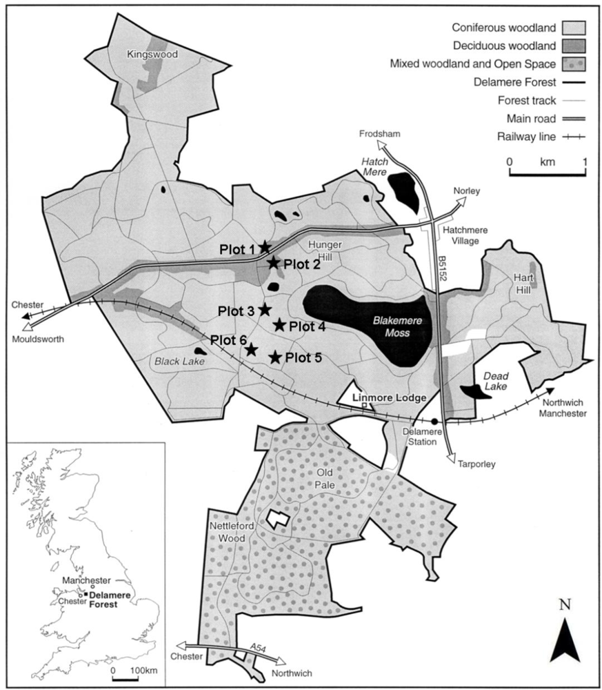
The study site chosen for this research was Delamere Forest, managed by the UK Forestry Commission and situated about 40 km south-west of Manchester (Figure 1). Delamere Forest is the largest area of woodland in the county of Cheshire covering a total area of 972 ha. Based on site inspections and stock maps of Delamere Forest provided by the Forestry Commission, three sampling plots were selected, composed of broadleaved deciduous, needle-leaved deciduous and needle-leaved evergreen trees respectively (

Table 1. Tree species found in the sampling plots chosen for this research.

Plot	Tree Species	Planted
Needle-leaved evergreen Plot 4	Corsican pine (Pinus nigra var maritima)	1945
Broadleaved deciduous Plot 3	Sweet chestnut (Castanea sativa)	1899
Needle-leaved deciduous Plot 5	Japanese larch (Larix kaempferi)	1981

) selected from six permanent sampling plots used for associated research (Figure 1).

The sensor used in this research was a Riegl LMS-Z210i, which is designed for the rapid and accurate acquisition of three-dimensional images by using a two-axis beam-scanning mechanism and a pulsed time-of-flight laser range finder. The data can be recorded by this sensor as either first return or last return of the signal backscattered from the targets, or a combination of both [3]. The TLS datasets collected for this research were recorded taking into account the first return of the signal backscattered from canopy elements. The Riegl LMS-Z210i has a beam divergence of 2.7 mrad and operates at a wavelength of 900 nm. The maximum range detected by the sensor is 650 m.

In order to capture the temporal dynamics of forest canopies, the TLS datasets for this research were collected on 3 April (leaf off), 13 May (leaf on) and 22 July 2008 (leaf on), and 19 March 2009 (leaf off). The data collection campaign was conducted using the methodology proposed by Danson et al.[3], which consisted of taking two orthogonal scans in order to capture most of the objects that are situated in the hemisphere above the TLS. The reason for this was that the sensor used in this research does not provide a full hemispherical coverage, as 80° is the maximum possible line scan angle. Spatially and temporally coincident TLS data and digital hemispherical photographs were acquired at the study site. The fieldwork was initiated by taking hemispherical photographs using a Nikon D70s digital camera with a calibrated full frame hemispherical lens (180° field of view across diagonal of photograph) orientated to look upwards. Once the photographs were taken, the TLS was mounted on a levelled surveying tripod, at the same height as the camera, and at an inclination angle of 90°. A single scan was taken with a line scan angle (zenith direction) of 80° and a frame scan angle of 330° (azimuth direction), using an angular sampling resolution of 0.108° in line and frame scan directions. The 3D information recorded by each scan was determined by the data acquisition parameters listed in

Table 2. Data acquisition parameters used with the Riegl LMS-Z210i (mounted at an inclination angle of 90°).

Line Scan Angle (Zenith Direction)
Start angle:	50°
Stop angle:	129.7°
Angular sampling resolution:	0.108°
Frame Scan Angle (Azimuth Direction)
Start angle:	15°
Stop angle:	345.4°
Angular sampling resolution:	0.108°
Additional Information
Number of returns obtained:	2,261,340
Acquisition time:	4 min

, set through the software RiSCAN PRO provided by the manufacturer. Table 2 also shows information relating to the number of points measured and the acquisition time.

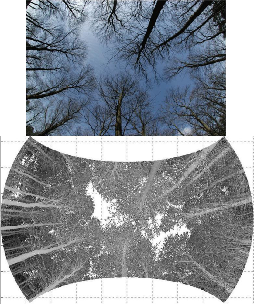
Figure 2 shows an example of a laser scanner image taken at the study site, generated by the data acquisition software, and its corresponding hemispherical photograph. Since the point size used to display the laser scanner image is not proportional to the actual beam footprint, the image appears to have significantly lower gap fraction than the hemispherical photograph.

4. Data Processing

In order to obtain estimates of canopy gap fraction, the hemispherical photographs taken coincident with the TLS measurements were processed with Caneye [5] software designed to extract canopy biophysical properties. The first step of the processing consisted of registering the photographs using a circle of interest of 60°, commonly used in gap fraction analysis, and an angular resolution of 5° in the zenith direction. Therefore, gap fraction distributions for twelve zenith bands (60°/5°) were computed. The second step involved the use of an interactive masking tool to eliminate regions of the photographs occupied by elements like sun glint, if present. In the third stage, the sky pixels, as well as those corresponding to plant elements, are determined by an automatic classification process. It is worth pointing out that there is a chance of having non-classified pixels after this stage, which requires manual intervention in order to classify them correctly. However, this can lead to errors in the classification, as there may not be clear distinction between sky and canopy pixels for certain regions in the photographs, which is very likely to be the case for an image acquired on a cloudy day.

For the TLS datasets, the x, y and z coordinates of canopy elements captured by the sensor were converted into spherical coordinates in order to obtain the range from the sensor to each of them with their corresponding zenith and azimuth angles. Subsequently, gap fractions for twelve 5° zenith bands (0–60°) were computed using the point-based method proposed by Danson et al.[3] and the intensity-based correction method (Equation (2)) described below. Again a circle of interest of 60° was considered to process the TLS data to enable comparison with hemispherical photography.

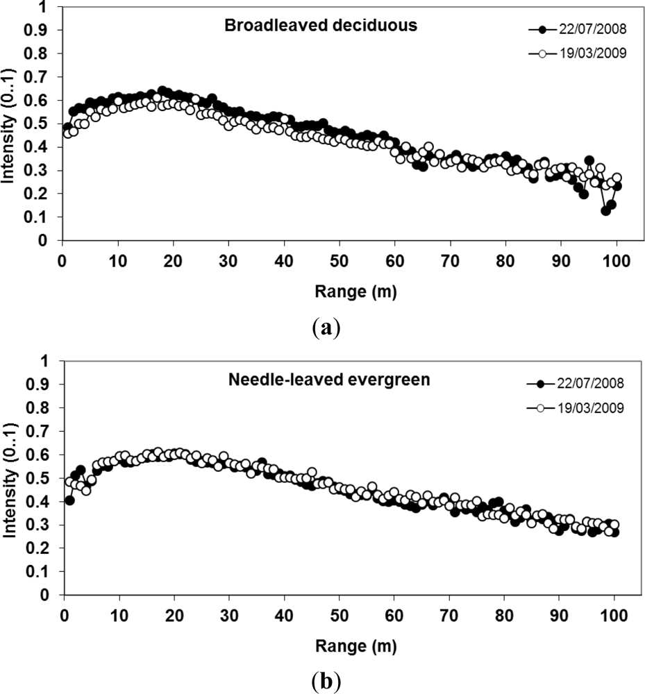
As examples, Figure 3 shows the maximum intensity values, found up to a distance of 100m, corresponding to TLS measurements taken at broadleaved deciduous and needle-leaved evergreen plots. With respect to datasets collected at the deciduous plot, maximum intensity values derived from the leaf on dataset were slightly higher than values corresponding to the leaf off dataset (Figure 3(a)). On the other hand, similar values are found in datasets acquired at the evergreen plot (Figure 3(b)). It is clear that the intensity variation in the region between 0 and 20 m was not in agreement with the inverse-square distance law presented in Equation (3), as the intensity values do not decrease with distance. Pfeifer et al.[25] conducted a series of experiments to test the agreement between intensity values measured by a TLS (Riegl 420i) and values predicted by the laser range equation. Intensity values were measured at different distances between the sensor and the targets selected. In general, a good agreement was found between measured and predicted values, except for measurements taken at very short (up to 2.5 m) and very long (beyond 20 m) ranges. In particular the measured intensity values increased up to a range of 2m, decreased between 2 and 20 m, and then increased again for longer ranges. The study concluded that this behaviour is related to the fact that the instantaneous field-of-view of the Riegl transmitter and receiver are not coincident, which has a larger impact on intensity values triggered at closer ranges. Since the range intensity response of the TLS used here was not known, and since it may differ from one instrument to another, it was necessary to implement an empirically-based instrument specific range-intensity correction.

The intensity-range correction process employed involved three stages: (i) from the set of return signals recorded by the TLS at each stand and each date, maximum intensity values were determined for each 1 m interval up to the maximum range detected by the sensor; (ii) the ratio i/I was calculated for all the return signals obtained, being i the intensity value recorded, and I the maximum intensity value found within the range interval at which i was triggered. At each interval, the value of I is assumed to correspond to a laser footprint that was fully intercepted by canopy elements. This assumption was necessary since there was no information on the echo detection algorithm implemented by the TLS system used in this research. Consequently, the percentage of the laser footprint that was occupied by canopy elements is given by the ratio i/I; and finally (iii) the corrected intensity value is given by the difference I-i.

Matlab™ code was written to implement these three stages. The difference computed in (iii) eliminates the range dependence of intensity values (Equation (5)). Thus, the gap fraction definition stated by Equation (2) can be re-written as:

$$\mathit{GF}=1-\frac{\sum \frac{i}{I}}{m}$$

(5)

where i refers to a given intensity value triggered within a given zenith band, I refers to the maximum intensity value found within the range interval at which i was activated and m indicates the number of laser hits expected within the given zenith band.

5. Results

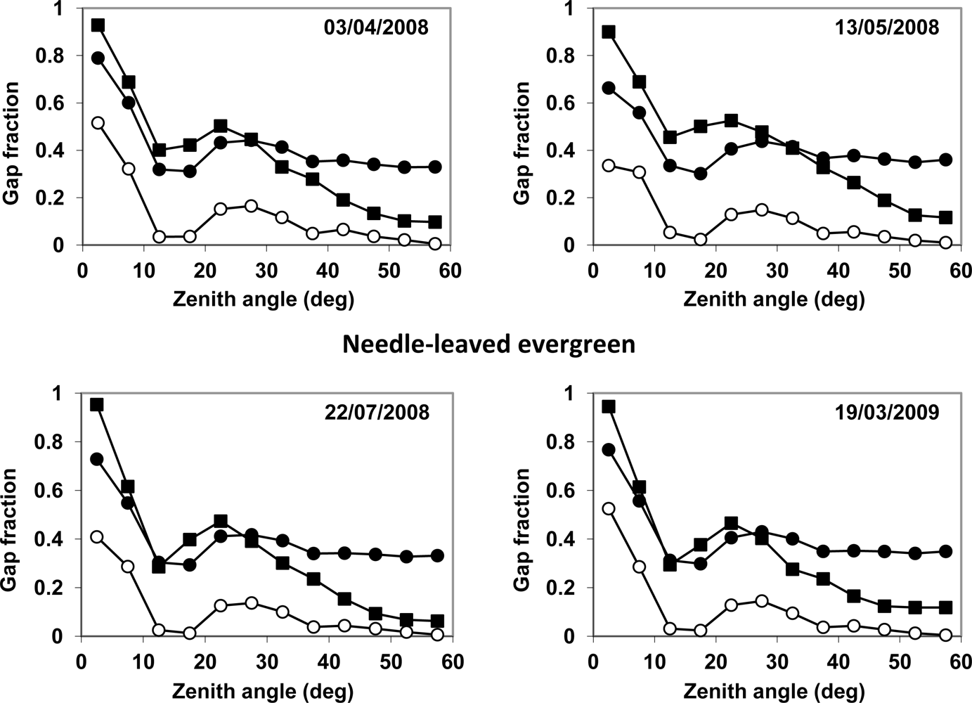
This section presents estimates of canopy gap fractions derived from the TLS measurements, calculated using both the point-based and intensity-based methods, and corresponding estimates obtained from hemispherical photography. The convention used in the following figures showing gap fractions is that estimates derived from the photographs (HP) are represented by solid squares, whereas solid and empty circles correspond to fractions calculated using the point-based (PB) and intensity-based (IB) methods respectively.

Figure 4 shows gap fractions derived from TLS measurements and photographs obtained at the needle-leaved evergreen plot and clearly indicates that gap fractions derived from the intensity-based method were larger than corresponding estimates obtained by the point-based method as would be expected. However, fractions derived from the intensity-based method showed closer agreement with the photographs than estimates obtained from the point-based method between zenith angles of 0° and 35°. On the other hand, fractions calculated by the intensity-based method between zenith angles of 35° and 60° were consistently larger than fractions derived from the photographs.

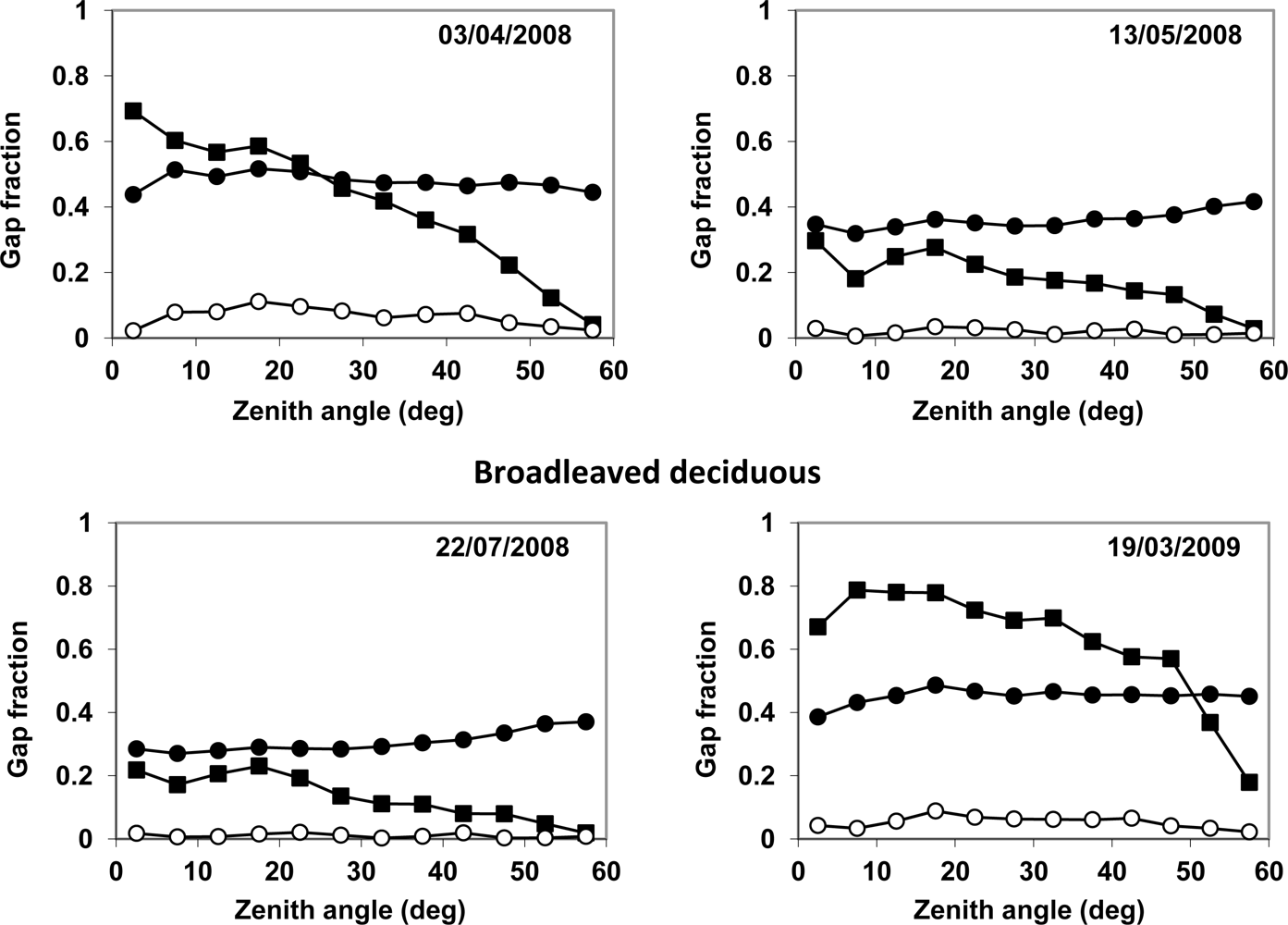
Figure 5 shows gap fractions derived from TLS measurements and photographs obtained at the broadleaved deciduous plot. For TLS measurements and photographs obtained on 3 April 2008, fractions derived from the intensity-based method were smaller than estimates obtained from the photographs between zenith angles of 0° and 35°. However, results obtained from datasets collected on 19 March 2009 indicate that estimates computed by the intensity-based method were consistently smaller than those derived from the photographs, except in the region between 55° and 60° zenith. As for datasets collected under leaf on conditions (13 May and 22 July 2008) the fractions derived from the intensity-based method were larger than corresponding estimates derived from the photographs. The figure also indicates again that fractions derived from the intensity-based method were larger than corresponding estimates obtained by the point-based method.

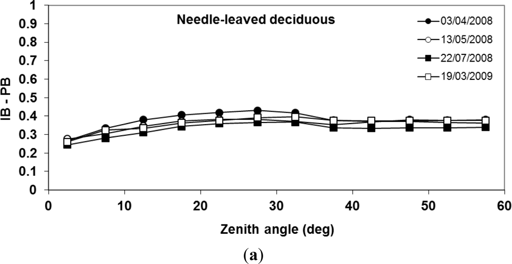
Figure 6 shows gap fractions derived from TLS measurements and photographs obtained at the larch plot (needle-leaved deciduous). For TLS measurements and photographs acquired under leaf off conditions (3 April 2008 and 19 March 2009), fractions derived from the intensity-based method were smaller than estimates obtained from the photographs between zenith angles of 0° and 35°. As for datasets collected under leaf on conditions (13 May and 22 July 2008), fractions derived from the intensity-based method were larger than corresponding estimates derived from the photographs. Figure 6 also indicates that fractions derived from the intensity-based method were again considerably larger than corresponding estimates obtained using the point-based method. This pattern was also observed in estimates derived from datasets collected at the needle-leaved evergreen and the broadleaved deciduous plots (Figures 4 and 5).

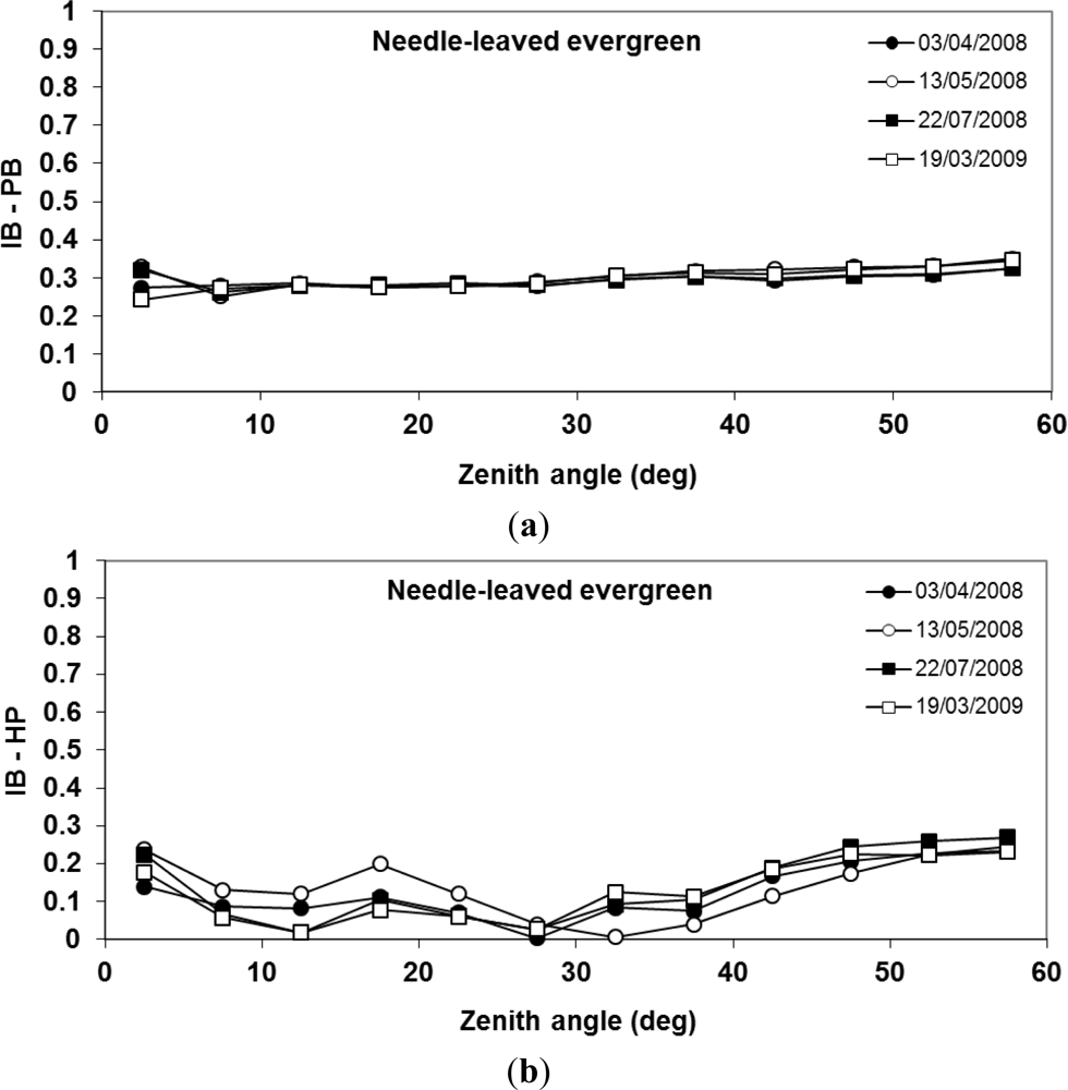
Figure 7(a) shows the differences in gap fractions derived from the intensity-based and the point-based methods at the needle-leaved evergreen plot where seasonal changes in gap fraction were expected to be small. The differences for the four dates were similar in magnitude, which is an indication of the repeatability of the TLS measurements. Differences between estimates derived from the intensity-based method and the photographs are shown in Figure 7(b). Similar trends were observed for all the datasets, especially in the region between 35° and 60° where fractions computed by the intensity-based method were consistently larger than corresponding estimates derived from the photographs.

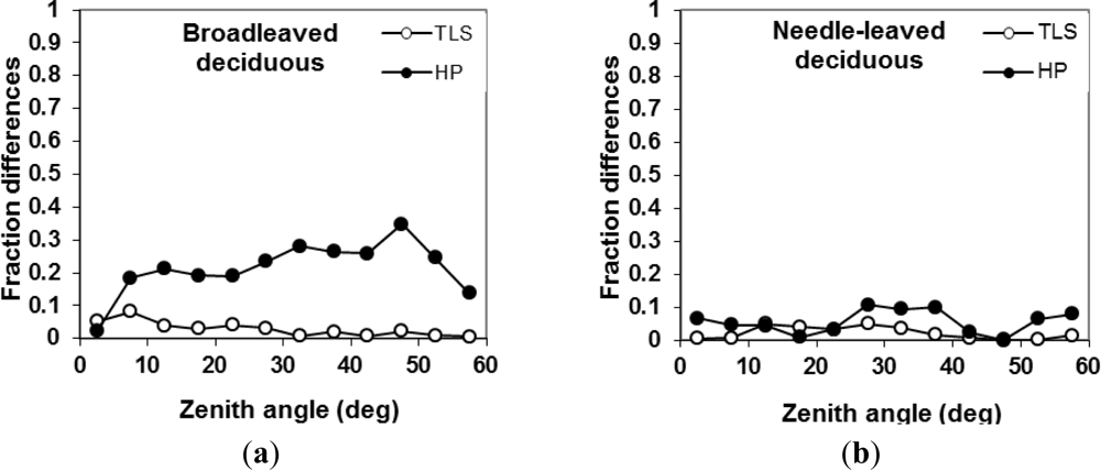
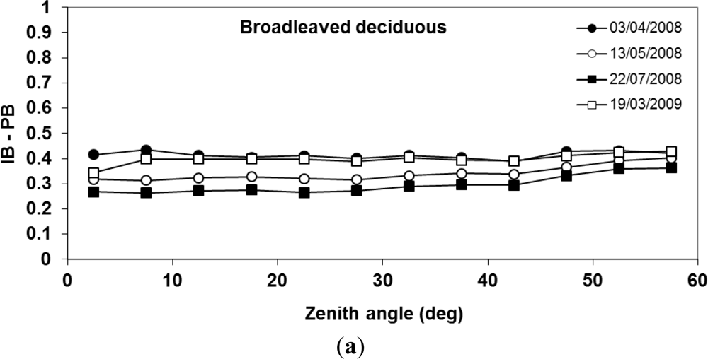
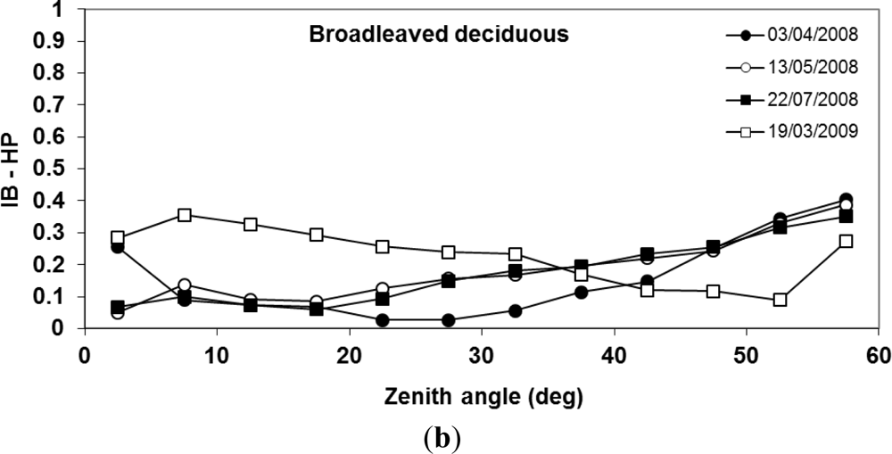
Figure 8(a) shows the differences in gap fractions derived from the intensity-based and the point-based methods for the broadleaved deciduous plot. For the datasets obtained under leaf off conditions (3 April 2008 and 19 March 2009) gap fraction differences were consistently larger than differences corresponding to measurements acquired under leaf on conditions (13 May and 22 July 2008). Differences between estimates derived from the intensity-based method and the photographs obtained at the broadleaved deciduous plot are shown in Figure 8(b), where similar magnitudes are observed for the leaf on datasets. For the leaf off data at 19 March 2009, larger differences up to a zenith angle of 40° were observed compared with the other datasets. However, the trend is the opposite for zenith angles larger than 40°, where differences were smaller for the 19 March data compared to the other datasets.

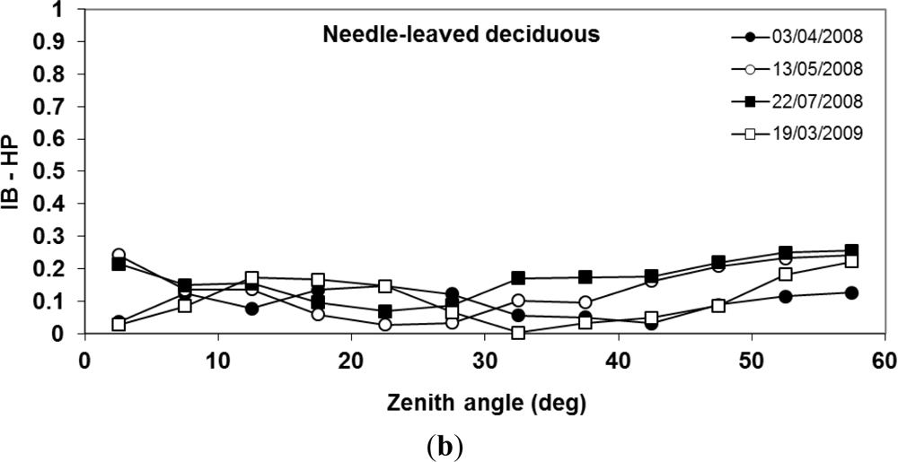
Figure 9(a) shows the differences in gap fractions derived from the intensity-based and point-based methods corresponding to the datasets obtained at the larch plot. The differences for the leaf off datasets were consistently larger than those corresponding to datasets acquired under leaf on conditions. Differences between estimates derived from the intensity-based method and the photographs (Figure 9(b)) were similar to those observed for leaf on datasets.

Table 3. Root mean square error (RMSE) of gap fractions obtained from both TLS methods versus gap fractions derived from the photographs.

	RMSE (%)	Needle-Leaved Evergreen	Broadleaved Deciduous	Needle-Leaved Deciduous
03/04/2008	PB v HP	27.81	39.01	42.26
Leaf off	IB v HP	14.15	19.75	10.00
13/05/2008	PB v HP	33.84	17.30	23.69
Leaf on	IB v HP	15.75	20.62	15.83
22/07/2008	PB v HP	27.49	13.89	17.93
Leaf on	IB v HP	16.45	19.73	17.93
19/03/2009	PB v HP	25.47	59.05	38.31
Leaf off	IB v HP	14.79	24.42	12.37

shows root mean square error (RMSE) values calculated using gap fractions derived from both TLS methods (point-based and intensity-based) and fractions obtained from hemispherical photographs corresponding to the complete set of Z210i measurements and photographs collected between April 2008 and March 2009. With respect to the datasets obtained at the needle-leaved evergreen plot, the values shown in the table confirm that estimates derived from the intensity-based method (referred to as IB in the table) presented a closer agreement with the photographs (referred to as HP in the table) in comparison with estimates obtained from the point-based method (referred to as PB in the table). For the intensity-based method the RMSE was less than 16.45% for all dates.

The measurements taken at the broadleaf deciduous plot indicated a closer agreement (though larger RMSE than for the needle-leaved evergreen plot) between fractions derived from the intensity-based method and the photographs in comparison with estimates obtained from the point-based method for the leaf off data sets. For the leaf on data sets the differences were smaller for the point-based method.

Finally, for the larch plot (needle-leaved deciduous) the intensity-based method again produced smaller gap fraction differences, compared to the photography, than the point-based methods at all dates. The differences were similar in magnitude to those observed for the needle-leaved evergreen stand but they were larger for leaf off dates.

6. Discussion

In general, the results presented indicate that gap fractions derived from the TLS intensity-based method were larger than corresponding estimates derived from the point-based method. The reason for this is that the point-based method takes into account the number of hits and misses recorded by TLS to compute gap fractions, but does not consider the portion of the laser beams not intercepted by canopy elements. This factor is taken into account by the intensity-based method and explains the difference in gap fractions derived from both approaches. In order to consider the empty portion of laser beams in the computation of gap fractions, it was necessary to make an assumption about the meaning of the intensity values recorded by the TLS. The assumption consisted of associating the maximum intensity values found at different range intervals to laser footprints that were totally occupied by canopy elements. The reason for making this assumption was the lack of information available from Riegl (the TLS manufacturer) on the echo detection algorithm, noise thresholding or range dependence of the intensity data for the TLS.

In comparison to estimates computed using the point-based method, gap fractions derived from the intensity-based method were closer in magnitude to corresponding results derived from hemispherical photographs. Nevertheless, in some cases TLS estimates were larger than results obtained from the photographs. Specifically, this was observed for leaf on datasets and photographs taken at the deciduous plots, as well as between evergreen datasets and photographs in the region between 35° and 60° zenith. These differences can be explained by the fact that at each range interval the intensity values are corrected with respect to the maximum value found within the interval. This implies that intensity values generated by foliage elements might then be corrected with respect to an intensity value triggered by a non-green (woody) element or vice versa. Here, the problem is that the assumption of the range correction approach was that there are no significant differences in the reflectivity of the material in the laser footprints; in the case of a mixture of woody and leaf or needle components, this assumption is unlikely to be true. Further investigation on the separation of canopy elements with different reflectance properties is necessary to avoid this effect.

For paired TLS datasets and photographs acquired under leaf off conditions (April 2008 and March 2009) no significant differences between gap fractions would be expected. However, Figure 10 indicates that noticeable differences were observed between results obtained from the photographs (represented by solid circles). On the other hand, estimates derived from the intensity-based method (represented by empty circles) present smaller differences highlighting the repeatability of the TLS measurements. Thus, the lack of repeatability of gap fraction measurements from hemispherical photography, due to differences in light conditions on the days when the photographs were acquired, may also have an impact on the measured difference between gap fraction estimates derived from both sources.

7. Conclusions

The comparison discussed in this research was carried out with the intention of obtaining a better understanding of the information that may be derived from TLS measurements and to use that information to develop a refined gap fraction extraction method. The results presented indicate that gap fractions derived from the intensity-based method can be used to characterise temporal dynamics in forest canopies. Moreover, gap fraction estimates can also be used to determine other biophysical properties of forest canopies, such as effective leaf area index and leaf area index, which also require information about the spatial aggregation of foliage elements characterized by the clumping index. However, the fact that TLS fractions obtained from leaf on datasets were consistently larger than results derived from the photographs suggests that more information may be needed to improve the corresponding gap fraction estimates. This indicates a limitation of the sensor used in this research, particularly the separation of green and non-green canopy elements. Separation of canopy elements with different reflectance properties is difficult because intensity is a function of both reflectance and the area of the object in the beam. The results derived from the intensity-based method underline the importance of intensity values recorded by TLS and show the potential for using this information to extract information on forest canopy structure. The use of this information requires a good knowledge of internal mechanisms that measure the intensity of laser returns. As the specification of those mechanisms was not available for the TLS used in this research, an assumption had to be made on the fraction of footprints covered by canopy elements by taking into account the intensity values and ranging information recorded by TLS. The match with gap fraction estimates derived from hemispherical photography may be improved by considering multiple returns that might be triggered for laser footprints with multiple partial hits within a canopy. Therefore, further development of the method presented in this paper is likely to require data from the new generation of full-waveform multiple wavelength laser scanners like the Salford Advanced Laser Canopy Analyser (SALCA) that has recently been developed by the authors [26].

When dealing with full-waveform systems, the intensity-based method will need to be reformulated in order to account for the information acquired by multiple returns. In this context, a single laser beam may produce multiple intensity values, which will be assessed based on the distance from the sensor at which they are triggered. The information captured by second, third and further returns will provide better characterisation of gap fractions, as a laser beam is partially intercepted by foliage or other elements as it travels through the canopy. If only the first return is taken into account, the portion of the beam that was not intercepted will be considered as a gap. However, as further returns may be triggered, the additional information recorded must be considered for the estimation of gap fractions.

Establishing a direct comparison between the TLS and hemispherical photography methodologies is problematic, as the analysis of hemispherical photographs is based on pixel classification, whereas the processing of TLS datasets involves the examination of patterns and distributions observed in the point clouds as well as the 3D information recorded by the TLS. In addition, results derived from hemispherical photographs depend on other factors such as illumination conditions and a manual intervention to classify the image pixels (sky and canopy elements). In contrast, active sensors like TLS do not depend on external sources for illumination and no manual intervention is required in processing the LiDAR measurements.

Finally, it is worth pointing out that the accuracy of gap fraction estimates derived from both TLS and hemispherical photography could be determined by making comparisons with manual measurements and destructive sampling. However, destructive sampling methods are exceptionally time-consuming and not applicable to this research, as they would have altered the plot conditions and prevented the detection of changes in the canopy. As an alternative to destructive sampling, a detailed structural model of a forest canopy could be developed by means of computer simulation, and the measured gap fraction derived from the virtual forest could be used to validate the TLS results.