Article

Surface Imprints of Water-Column Turbulence: A Case Study of Tidal Flow over an Estuarine Sill

by
George O. Marmorino
*,
Geoffrey B. Smith
and
W. David Miller
Remote Sensing Division, Naval Research Laboratory, 4555 Overlook Avenue S.W., Washington, DC 20375, USA
*
Author to whom correspondence should be addressed.
Remote Sens. 2013, 5(7), 3239-3258; https://doi.org/10.3390/rs5073239
Submission received: 5 May 2013 / Revised: 25 June 2013 / Accepted: 26 June 2013 / Published: 4 July 2013
(This article belongs to the Special Issue Observing the Ocean’s Interior from Satellite Remote Sensing)

Abstract

:
Turbulent mixing in the ocean can, in some cases, be so intense as to leave surface imprints, or “boils”, that are detectable from space. Examples include turbulent flow over a submerged obstacle and instability of large-amplitude internal waves. In this paper we examine the particular case of tidal flow over a ∼60-m-deep sill, which forms a barrier for the flow of dense water from the Pacific Ocean into the Strait of Georgia. The flow response during flood tide is illustrated using visible and thermal-band satellite and airborne imagery, the latter having high-resolution multi-looks that capture the formative stage of the boils. The image examples capture aspects of the expected flow response based on in situ measurements reported in the literature, but they also suggest differences, and they reveal the level of complexity of the surface structure. A new result is that, after the front is pushed well off the sill, boils emerge several hundred meters downstream from the sill crest, grow at a rate of ∼60 m2/s, and attain a size of 3,800 m2 (an equivalent diameter of 70 m) after one minute. These boils appear to arise from vorticity generated by vertical shear at the sill crest, and provide an additional source of vertical mixing and (through wave breaking) air-sea gas exchange.

Graphical Abstract

1. Introduction

Ocean turbulence is an energetic, eddying state of motion that disperses material and transforms momentum at rates far higher than those of molecular processes alone; an understanding of how turbulence is produced and its nature and effects in shallow seas, the deep ocean, and in the mixed layer is consequently of considerable importance and practical application [1]. The larger-scale coherent structures associated with ocean turbulence can produce surface (or near-surface) signatures that can be detected using remote sensing techniques and used to infer ocean parameters. An example is using the spacing of Langmuir turbulence to deduce the depth of the mixed layer [2]. Some flow instability processes can generate localized ejections, or bursts, that transport momentum and small-scale turbulence upward from a source deeper in the water column. These bursts impinge on the sea surface to produce structures described as boils. In a boil, water brought to the surface from below spreads on the sea surface in a patch of diverging motion. The diverging flow leads to a surrounding, sometimes near-circular, band of surface convergence and downwelling motion. Within this band, wave-current interaction results in the steepening, and often breaking, of short surface waves; and this leads to the generation of air bubbles that are trapped by the converging currents. Blocking of ambient surface waves leads to a smoother sea surface in the diverging part of a boil. The boils thus have a distinctive pattern in the distribution of small-scale wave slope, or surface roughness, which is detectable in sunglint and synthetic aperture radar imagery. Also, as the upwelled water in a boil may differ from the ambient surface water in both optical properties and temperature, boils can be expected to have signatures in both ocean color and thermal infrared (IR) imagery.
Boils have been reported for relatively weak stratification in a shallow tidal sea (water depth about 45 m) [3,4]; in a 200-m-deep estuary [5]; over 25-m-deep sand waves [6]; and downstream of 4-m-deep sills [7,8]. Boils have also been reported in association with a headland-induced front [9,10] and with large-amplitude internal waves [11,12]; and boils can be expected to occur in other situations, as well, e.g., in association with upwelling of buoyant outflow water at the edge of an ice shelf. The present paper uses a limited set of visible and IR satellite and airborne imagery to investigate the case of tidally forced flow over a ∼60-m-deep estuarine sill. Specific questions addressed in this paper are as follows: Are boils captured in thermal imagery? How useful is thermal vs. visible imagery? Can time and spatial scales of the turbulent structures be derived from imagery? Is the imagery consistent with the existing physical framework for the flow? Can a specific dynamical link be established between boils and the sill flow? What issues need further study?

2. Approach

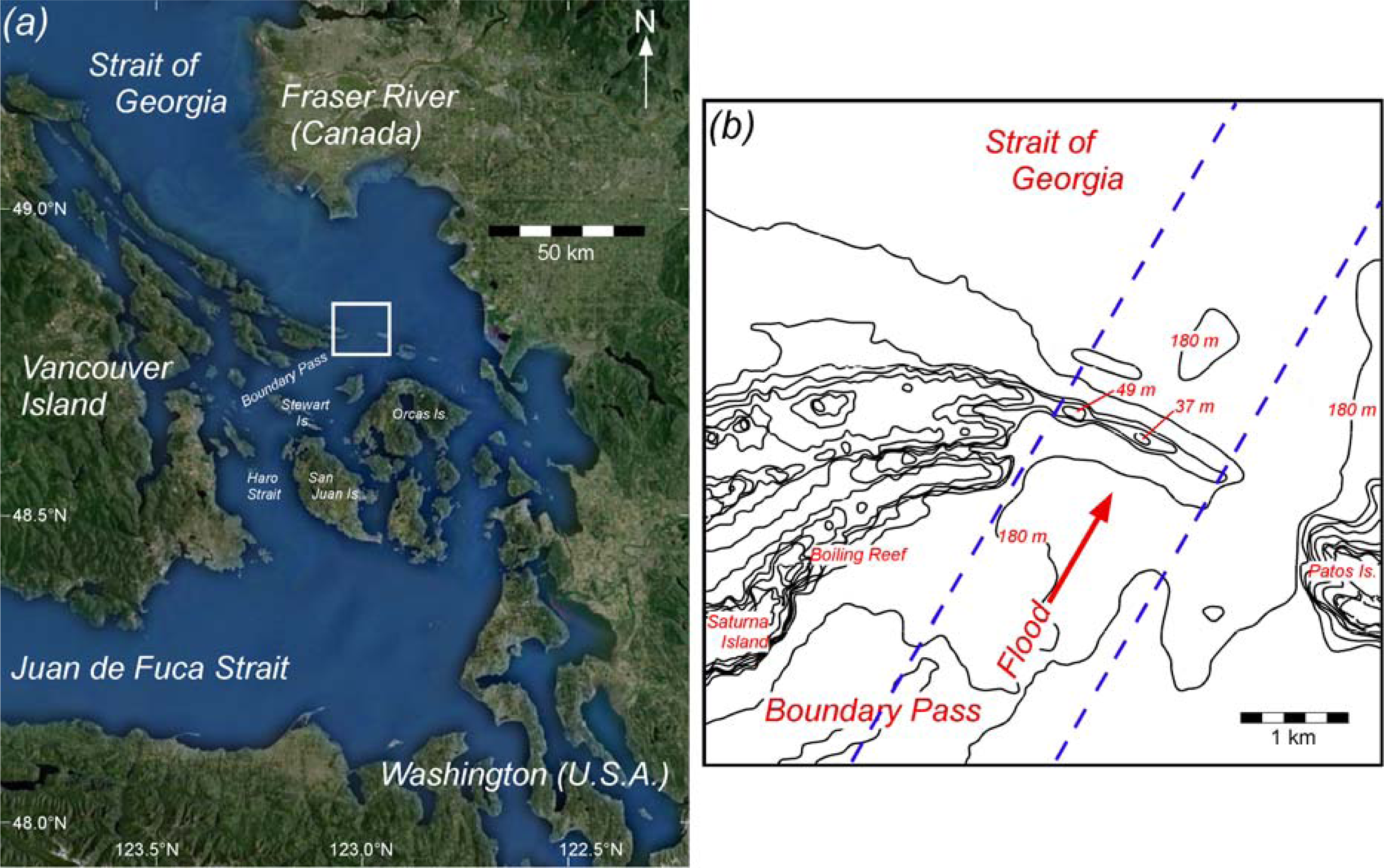
2.1. Study Site Background

Haro Strait, along with the Strait of Georgia and Juan de Fuca Strait (Figure 1), form an estuarine system dominated by two water masses: a thin buoyant surface layer originating in the Fraser River plume and a deep saline layer originating in the Pacific Ocean. Vertical mixing between the surface and deep layers amplifies the volume flux in each layer, making it important to identify the processes doing the mixing, and where and when they occur. Two sills dominate the bathymetry in Haro Strait: Victoria sill at the southern end and a sill at the northern end of Boundary Pass, which is the focus of the present paper. The presence of these sills has led to the hypothesis that a process known as hydraulic control (and the turbulence generated in a hydraulic jump downstream of the control) may be important [13].
The Boundary Pass sill lies between Saturna and Patos Islands (Figure 1(b)). The sill rises from a depth of about 200 m to 60 m and has a mean slope of 30°. During flood tide, the current, which can reach speeds of up to 3 m/s, forces dense water from Boundary Pass over the sill (and partly through the gap at the eastern end of the sill) into the Strait of Georgia. In situ measurements reported by Baschek et al. [13,14] have elucidated various physical processes active near the sill on flood tide (Figure 2). Guided by internal hydraulic theory [15,16], Baschek et al. [13] divide the flow response into two distinct stages of forcing: “strong” and “extreme”.
The strong forcing stage, in which the flow is hydraulically controlled by the sill, occurs 0.5 to 1.5 h after ebb slack. In this stage, dense water advects over the sill and then subducts beneath an arrested, wedge-shaped, buoyant, upper layer comprised of Fraser River plume water. Subduction occurs along a plunge line, or tidal convergence front, which is offset 100 m or so downstream of the sill crest [13,17]. The convergence front is marked by a 50-m-wide zone where surface waves, shortened and steepened by the current gradient, break and aerate the surface water. The air bubbles are then swept beneath the front and help ventilate the deep and intermediate water in the Strait of Georgia, giving the front an important role in air-sea gas exchange [13]. The lower-layer flow follows the bathymetry to the bottom of the sill, where a hydraulic jump marks the transition to subcritical conditions. A velocity section reported by Baschek et al. [13] shows the jump at a depth of 170 m and at a distance of 350 m from the sill crest. Detrainment of lower-layer fluid into the buoyant upper layer can manifest itself as 50-m-sized overturning cells at 50- to 100-m depth [14].
The extreme forcing stage occurs 2.5 to 4.5 h after ebb slack and encompasses peak flood current. Now, the flow separates from the sill crest as a high-speed jet, and the plunge line is pushed far downstream and becomes less distinct. Energetic boils can occupy a region from several hundreds of meters to two kilometers downstream of the sill; and the horizontal extent of the associated upwelled water can exceed 100 m, as can be inferred from sections of acoustic backscatter intensity reported by Baschek et al. [13]. A possible source of the turbulence may be shear instabilities associated with the jet [18].
An additional part of the dynamics of flow over a pronounced submerged obstacle such as a sill is the generation of internal waves [1820]. While the energetics have not been specifically addressed for the Boundary Pass sill (but see [21]), studies of similar sill flows show the bulk of the loss in barotropic tidal energy is radiated away as internal waves, while the remaining energy loss is to processes occurring near the sill, e.g., through the generation of small-scale coherent structures [19]. Internal waves believed to originate at the Boundary Pass sill have been observed in Georgia Strait [22,23], but in the far-field, well downstream of the region shown in Figure 2. Also, during “intermediate” tidal forcing [15,17], buoyant surface water can occur upstream of the sill [14], so that the flow response may include upstream effects such as internal jumps and solibores [19,20] (Representative temperature and salinity profiles at Boundary Pass can be found in reference [24]).

2.2. Satellite Imagery

Only a handful of examples during flood conditions were found in the publicly available imagery archives of ASTER and LANDSAT, both of which have a thermal band. We chose a LANDSAT Enhanced Thematic Mapper Plus (ETM+) scene from June 2000 (Table 1), so as to be seasonally close to the airborne dataset described below. The image time corresponds to 0.1 h into the strong forcing stage, and the predicted current at maximum flood was 1.1 m/s. Bands 1–3 (450–520, 520–600, and 630–690 nm) were used to construct an RGB visible image having 30-m resolution. Band 6 (10.4 to 12.5 μm) provides the thermal image having 60-m resolution; temperature resolution is of the order of 0.3 °C. LANDSAT views at nadir (±7.5°); the sun elevation at the time of the data acquisition was 59.7°.
For a second example, we include a GeoEye-1 pass collected in July 2012 (Table 1), which was the only higher-resolution imagery we could find of the area during flood tide. The image time corresponds to 1.7 h after slack, just 0.2 h after the end of strong forcing; the maximum flood current is 1.0 m/s, in this case. GeoEye-1 provides 1.65-m resolution multispectral data (bands at 485, 560, and 660 nm are used here) and 0.41-m panchromatic data. GeoEye-1 has an altitude and data swath similar to LANDSAT 7; sun elevation at the time of the data acquisition was 61.3°.

2.3. Airborne Measurements

Thermal imagery was collected using a mid-wave infrared (IR) camera (Merlin-Mid, Indigo Systems/FLIR, Wilsonville, OR, USA), which was flown aboard a de Havilland DHC-6 Twin Otter aircraft. The camera operates in the 3–5 μm wavelength band, has a frame size of 320 by 256 pixels, a 40° field of view (13-mm camera lens), a sample rate of 60 frames per second, and an NEΔT (noise equivalent temperature difference) of 0.017 °C. The IR camera was mounted on a computer-controlled gimbal, usually fixed in position to provide nadir view. These fixed-view data were processed by using the center row of data from each raw IR image to build-up an image strip, which is then geo-referenced as for a push-broom sensor. The accuracy of the resulting geo-strip data is about 10 m. Some IR data were also collected in “staring mode”, in which the same ocean scene can be viewed continuously for several tens of seconds. This was done by aiming the camera far forward as an area of particular interest is approached, then continuously adjusting the look-angle to keep that area in view as the aircraft flies first over and then forward of the target area, after which the gimbal is reset for continued nadir viewing. Rapid adjustment of the gimbal between staring and nadir-viewing modes can result in a localized glitch in a geo-strip, which may be apparent in some of the figures.
Flights over the Boundary Pass sill were conducted on the night of 17 May 2009, beginning at the start of flood tide and with the intent of continuing through the end of the extreme forcing stage. Measurements were cut short, however, by encroaching low-level clouds, and only 2.2 h of data could be collected. In all, 15 passes were done from 0.1 to 2.3 h after slack tide (Table 1), corresponding to 0.4 h before strong forcing stage to 0.8 h after; the maximum flood current was 1.0 m/s. Aircraft altitudes were either 1,525 or 3,050 m, resulting in IR image swaths of 1,130 or 2,255 m and spatial resolutions of 3.5 or 7.0 m. The imaged area is indicated in Figure 1(b) by the dashed blue lines that are oriented normal to the sill and along 30°T. Because of the orientation and narrowness of the image swaths, all the aircraft data are presented in a more convenient rotated frame with the image geo-strips vertical on the page.
Some additional IR data were acquired during daytime on 23 May (Table 1). In this case, visible-band data were also collected using a Compact Airborne Spectrographic Imager (CASI) (CASI-1500, ITRES, Calgary, AB, Canada), a pushbroom sensor having a 40° field of view and 1,500 across-track pixels. Aircraft altitudes were either 1,680 or 580 m; image swaths, 1,220 or 425 m; and spatial resolutions, 0.81 or 0.28 m. The CASI data were collected in 36 bands, between wavelengths of 380 and 1,048 nm. Images shown in this paper use bands at 648 nm (red), 552 nm (green), and 457 nm (blue). Data were collected near local noon, and sunglint was an issue because of the high sun elevation. Glint was reduced in the visible data following the procedure described by Hedley et al. [25]. The effect of sunglint in the mid-wave IR band was minimized by using the gimbal to view away from the sun. As a result, IR and visible sensors often had offset looks, resulting in the same area of sea surface being viewed at slightly different times.
On both 18 May and 23 May, solar heating under clear skies can be expected to have produced a diurnal warm layer, while net surface cooling resulted in a “cool skin”, meaning the undisturbed sea surface is cooler than the immediately underlying water. These effects were estimated using a bulk air-sea flux algorithm [26] along with meteorological measurements made at East Sound, Orcas Island (Figure 1(a)). The calculated temperature difference across the warm layer was ∼2.8 °C on 18 May and ∼0.3 °C on 23 May; and the thickness of the warm layer was of the order of 1 m and 10 m. The calculated temperature drop across the cool skin was small on both days (∼0.09° and 0.03 °C); and the thickness of the cool skin was 3.6 and 1.2 mm. The warm layer can thus be expected to have greater significance for the thermal signatures of boils.

3. Results

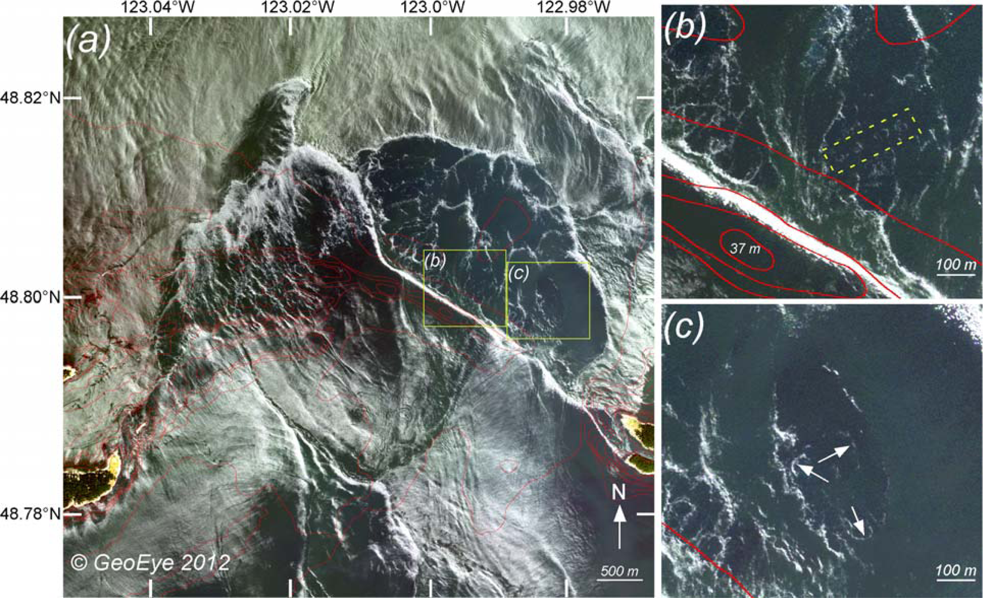
3.1. Satellite Imagery

The most prominent feature in the LANDSAT scene (Figure 3) is a temperature and color front that extends to the northeast from Boiling Reef, an area of shoals at the end of Saturna Island (Figure 1(b)). The front marks the northern edge of a widening band of cooler water that derives from turbulent mixing over the shoals and sill. Evidence for this interpretation is small-scale structure within the band that can be seen in both the visible and IR images, and which also appears in the second satellite image discussed below. Water 2.2 °C colder than the surrounding surface appears in two approximately circular areas (diameters ∼200 m) that occur about 600 m downstream of the sill (within the red box in the figure) and which we can tentatively identify as large boils. In the visible image, the boils appear as bright outlines, resulting from enhanced sunglint, consistent with wave-current interaction along the perimeter of the boils. Somewhat difficult to see in Figure 3(a) is a narrow, bright line that runs very near the sill crest (the dashed yellow curve in the figure). This signature is evidence of the wave-current interaction zone along the frontal plunge line (e.g., Figure 2(a)), and its location is consistent with the imagery having been acquired during the strong forcing stage of flood tide.
The GeoEye imagery (Figure 4) shows the visible phenomena much more clearly. There is a wave-current interaction zone (the straight white band) located about 100 m downstream of the sill crest, indicating the position of the tidal convergence front. The zone has a width of about 50 m (Figure 4(b)), consistent with in situ observations (Section 2.1). The front bends northward where the sill begins to broaden in the west, and it weakens where it encounters the surface turbulence from Boiling Reef. The bend suggests a plunge line that has been pushed downstream by the currents (e.g., Figure 2(b)), which is possible as tidal forcing typically leads over shallower water. The front also extends eastward toward Patos Island, which is unexpected. The occurrence of a front there, in the constrictive gap between the sill and Patos Island, suggests the possibility of a different kind of response, as flow through constrictions can also result in frontogenesis [15,17]. Northeast of the sill, the image suggests a large area of surface turbulence, consisting of shapes of various sizes. Examples include a line of five ∼20-m wide boils (shown enlarged in Figure 4(b)) and a 100- by 200-m oval-shaped area (Figure 4(c)) that is relatively dark compared with the surrounding water and shows evidence of smaller-scale boil activity. Similar turbulent-like patterns extend 1.6 km downstream from the sill, ending abruptly where the water’s color changes to a more greenish hue, representing the Fraser River plume. The image texture changes dramatically here, as well, glint patterns north of this color front resembling internal waves rather than turbulence. Analogous texture and color changes occur in the LANDSAT image.

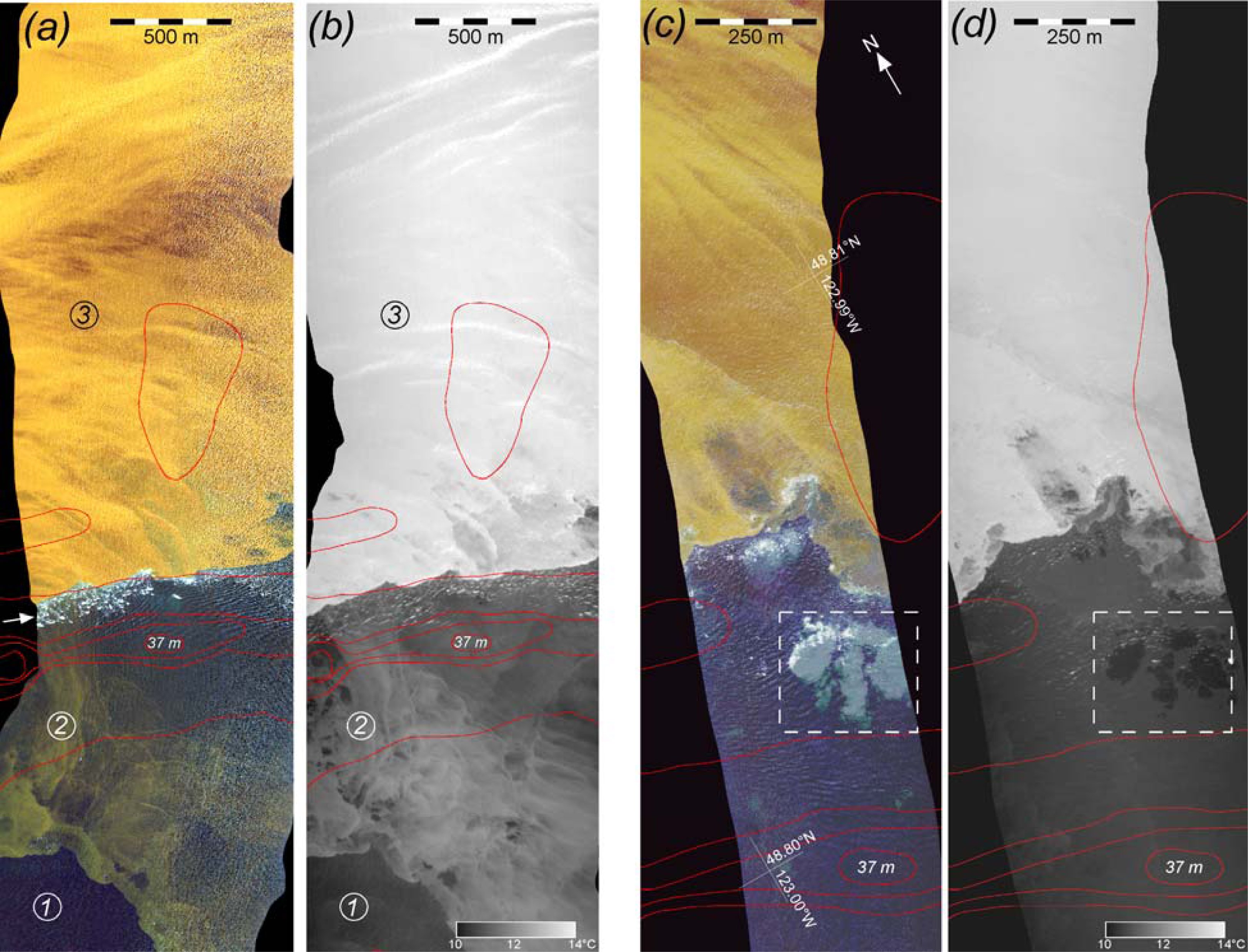
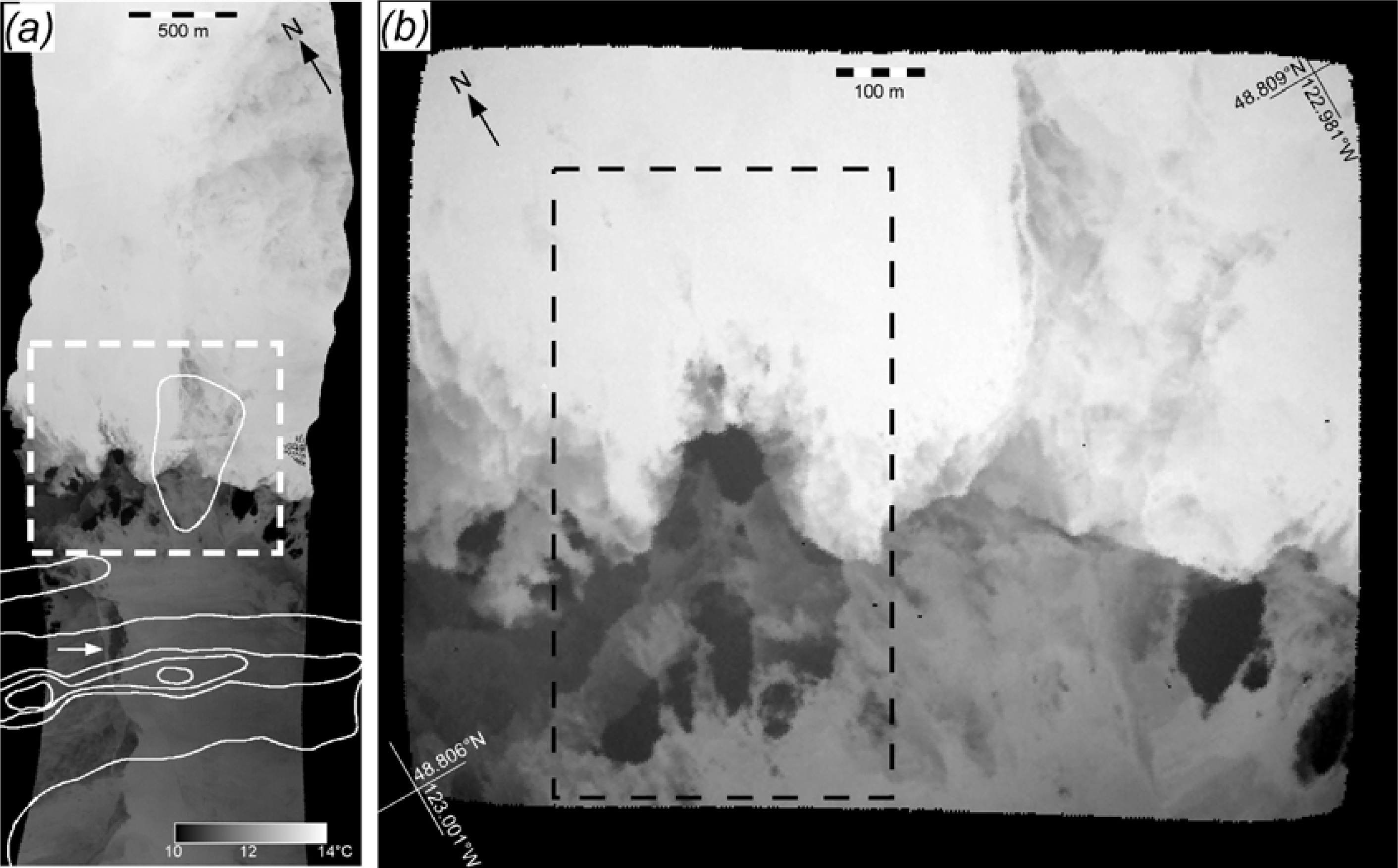
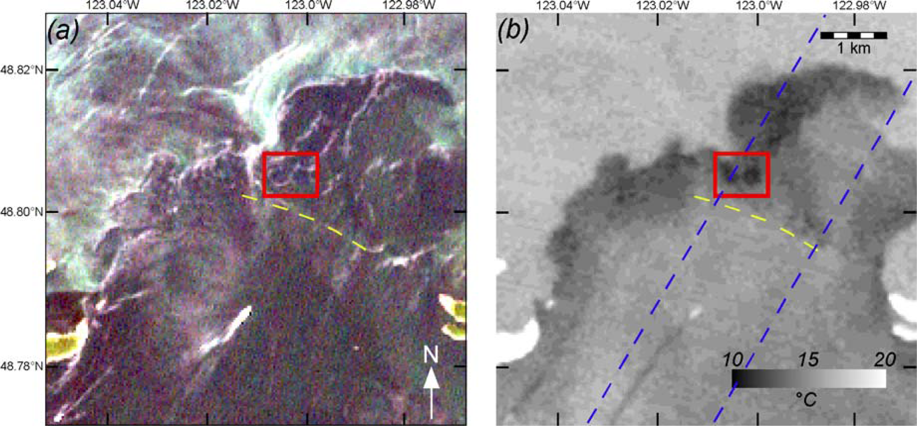
3.2. Daytime Aircraft Imagery

Coincident visible and IR airborne imagery present a common view of a range of phenomena (Figure 5). (Note that, as a result of the IR camera being angled forward, there is a small time offset between the visible and IR views.) A first pass (panels (a) and (b)) was made ∼0.7 h before the start of strong forcing; nevertheless, clear, coincident temperature and color fronts lie near the sill crest. A wave-current interaction zone appears in the visible image (arrow, panel (a)) and to a lesser degree in the IR image through reflected solar IR radiation. An additional front lies ∼1 km south of the sill (bottom left in the figure). This front separates relatively clear (blue) and cooler water (type 1 in the figure), representative of well-mixed Haro Strait water, from turbid (yellow-green) and warmer type-2 water, possibly remnant plume water from the previous ebb tide. This type-2 water is filled with narrow, curved bands that are warmer and greener than the surrounding water, and which we presume to be internal wave troughs. Many of these have scum lines along their forward edges, which would be consistent with converging currents at the leading edge of a wave trough. Vertical mixing embedded within the internal wave field is suggested by areas of numerous small, cool patches (perhaps small-scale boils) that coincide with spots of relatively clear water in the visible image. Internal wave signatures also appear in the plume water north of the sill front (type-3 water), e.g., a group of bright bands near the top of the IR image (Figure 5(b)) show a wavelength of about 100 m and coherence lengths of up to 1.5 km.
A second pass (Figure 5(c,d)), made 24-min later, shows the front displaced well downstream of the sill and having pronounced cusps, small-scale swirls, and across-front intrusions. There is no wave-current-interaction zone over the sill as in the first pass. South of the front the water is generally clear (blue) and cold. Between the front and sill is a cluster of boils (area of dashed rectangle). These appear in the IR image as cold patches (about 0.4 °C cooler than ambient), and in the visible image as brighter patches with areas of wave breaking and foam, primarily along the upwind (north) edge of the boils. (See below.) Spectrally, the visible boil area shows enhanced reflectance in the green wavelengths of about 500 to 550 nm as compared with ambient water surrounding the boils (Figure 6). This green-shift is characteristic of light backscattering from large “clouds” of air bubbles [27]. Further evidence for bubbles is a close agreement between spectra from the boil areas and spectra from the bubbly part of the wake behind a large tanker (Figure 6). (The tanker was imaged in a separate pass flown at 300-m altitude in the area south of the sill.) The visible boil signatures thus arise from bubbles; the IR signatures from disruption of a warm surface by cold water from below. As the boils occur between the sill and the downstream-displaced convergence front, the water column is likely weakly stratified. The boil thermal contrast (∼0.4 °C) should then be determined primarily by the temperature change across the diurnal warm layer, which is about 0.3 °C (Section 2.3).
A detailed comparison of the boils shows that the visible signatures (Figure 7(a)) tend to be spatially more extensive than the thermal imprints, which were viewed ∼9-s earlier (Figure 7(b)); one area in particular, visible patch E, has no thermal expression at all. An explanation is that the visible signature in some areas represents a completely submerged bubble cloud that only subsequently impacts the sea surface. Thus, we propose that the thermal imprints continue to form and grow over the 9-s interval between panels (a) and (b). Direct evidence for such growth is provided by an examination all the IR frames that contain the boils. (This is possible because the high framing rate of the camera greatly over-samples every scene.) Two of these frames (Figure 7(c,d)) were acquired 4 s before and after the IR data shown in Figure 7(b). Figure 7(c) shows the boils first entering the camera’s field of view, and so the boils appear near the top edge of the frame; Figure 7(d) shows just the opposite. By comparing the three IR panels, it can be seen that cold imprints grow over time and fill-in some of the ‘missing’ parts within the red outlines. For example, two small cold spots (features 1 and 2) grow within visible patch D, increasing in area at a rate of roughly 20 m2/s. A conjecture is that this growth arises from the surfacing of parts of a large volume of subsurface turbulence, as represented by the larger submerged bubble cloud.
But how do bubbles become distributed over an entire patch when breaking waves and bubble injection are localized (e.g., Figure 7(a))? Here it is important to remember that the visible image is a snapshot, while the bubble distribution being portrayed is the result of an evolution over time. Our view is this: Bubbles may be injected locally, but they are quickly distributed over a large subsurface volume by turbulent eddies. The resulting submerged bubble mass can be sustained against a divergent surface flow. Also, as more turbulent eddies in the upwelling water rise closer to the surface, new “interior” boils emerge, and these create new wave-current interaction zones and new sources of bubbles. Evidence for this viewpoint can be found in some of the imagery. For example, the GeoEye image (Figure 4(c)) shows several semi-circular bright arcs that we presume to be the expanding perimeters of interior boils. An alternative hypothesis is that the bubble patches derive from bubbles injected at the tidal front, and are then recirculated through the water column to their observed upstream frontal location through a flow-separation eddy as in Figure 2(b); but this explanation seems far less likely, in our opinion.

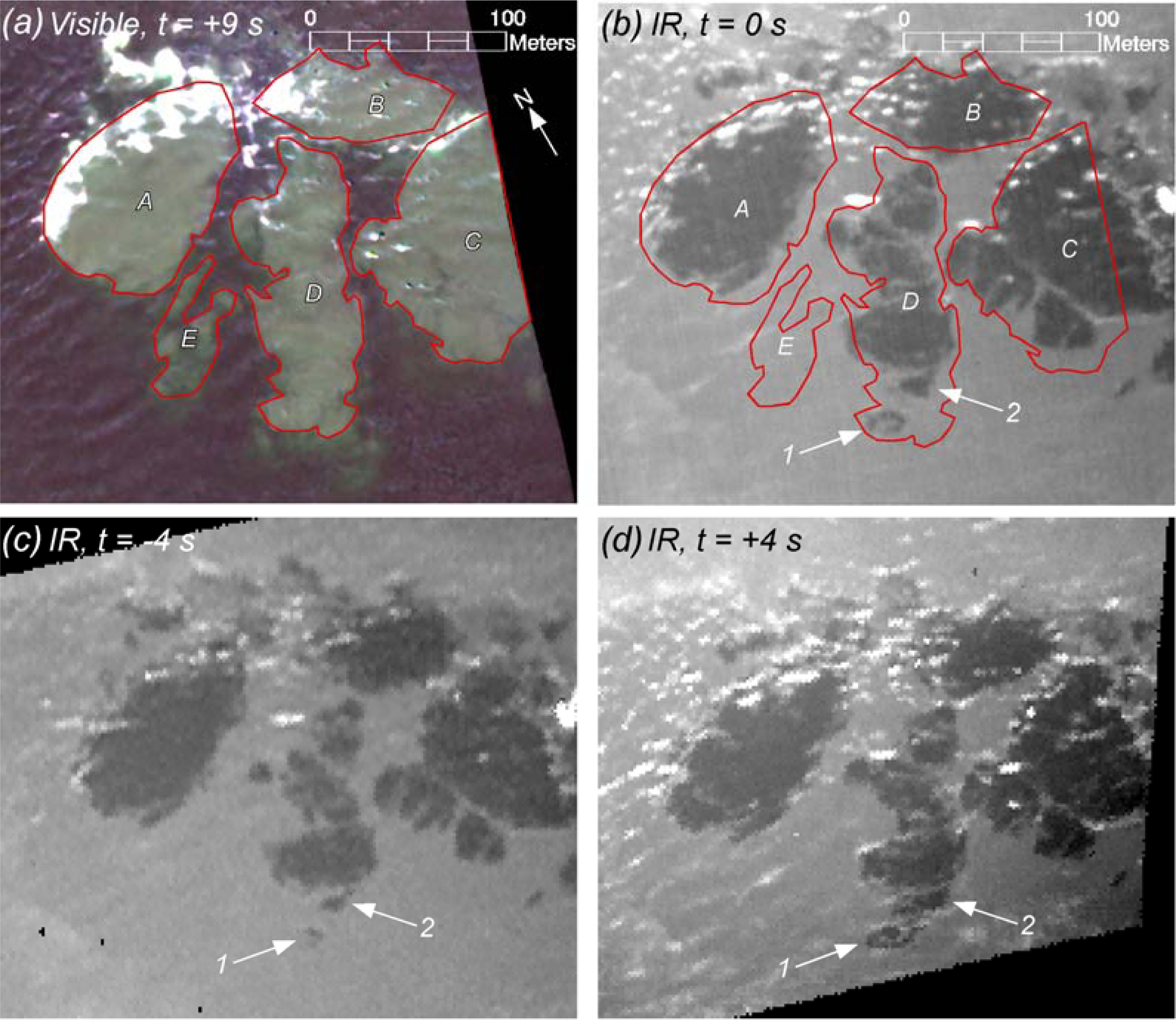
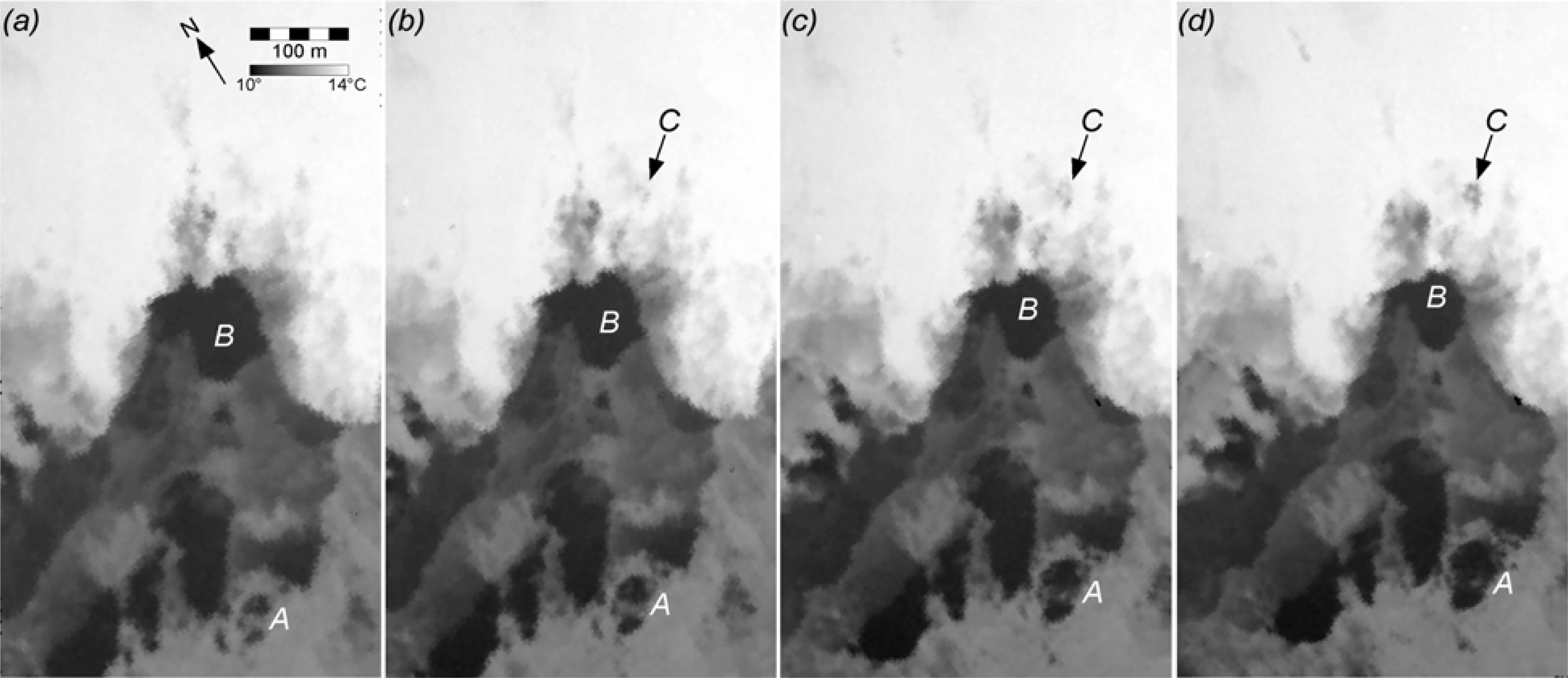
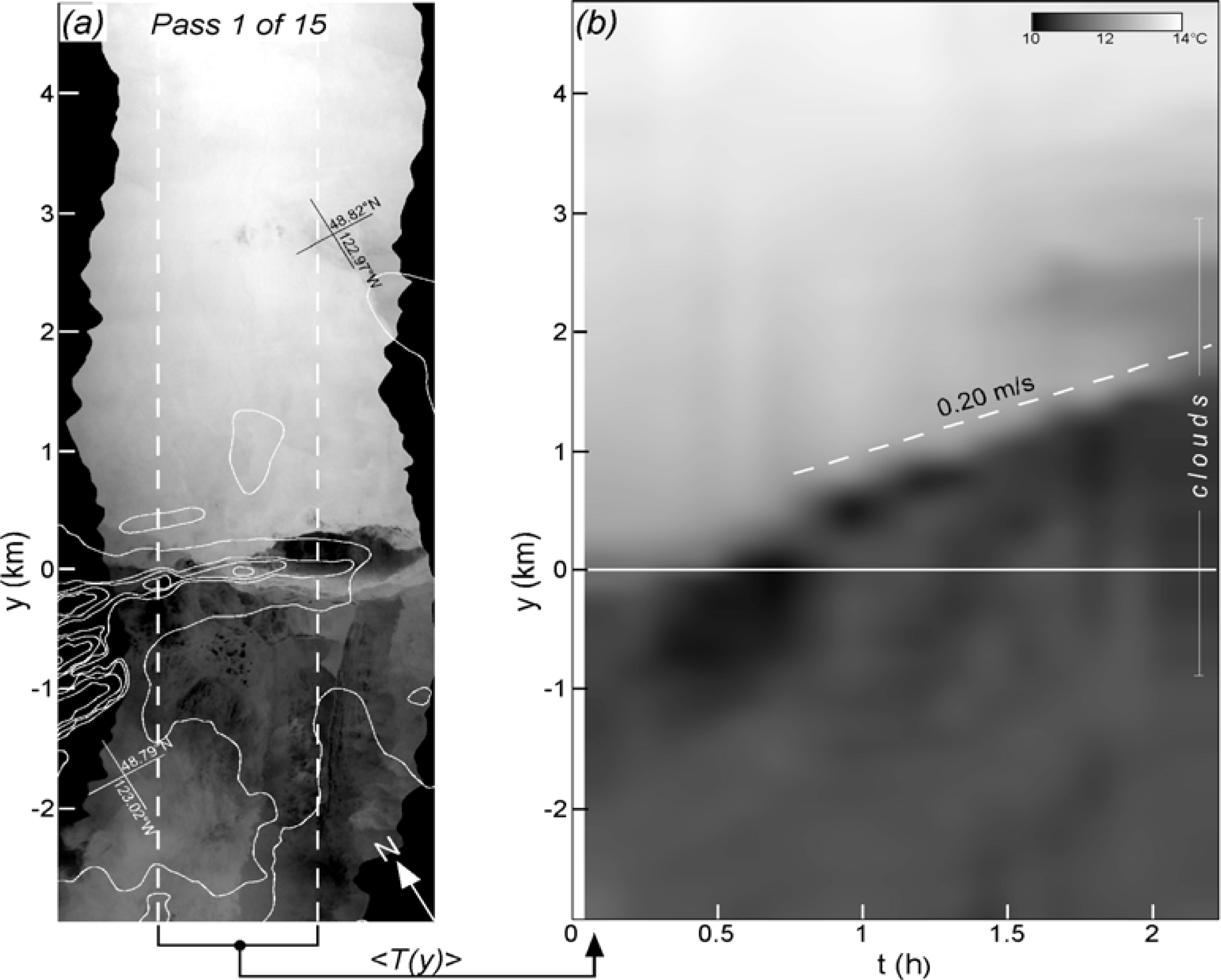
3.3. Nighttime Aircraft IR Imagery

A view of the continuous evolution of the thermal field over 2.2 h is provided by the nighttime data collected on 18 May. The first of 15 available passes is shown in Figure 8(a) as an example. This corresponds to 0.4 h before the start of strong forcing, and conditions upstream of the sill show evidence of the same stratified dynamics (internal waves and areas of small-scale mixing) seen in the daytime image (Figure 5(b)) at 0.7 h before strong forcing. A new feature is a pronounced warm band that extends upstream (and west) of the sill crest, so that an elongated oval-shaped area of colder water lies between it and the warm front of the stagnant layer. This feature is approximately stationary for ∼0.3 h, after which it breaks down. The feature resembles a “breaking” internal wave [28], developing as part of the time-dependent response of the flow. The evolution of the across-sill temperature field (Figure 8(b)) shows the initial trapping of the tidal convergence front to the sill. Subsequently, the front moves steadily away from the sill (mean speed about 0.20 m/s), and the area between the sill and front cools relative to the water upstream of the sill. This is consistent with boils forming downstream of the sill (see below). Toward the end of the period shown in Figure 8(b) (t > 1.5 h) a cooler region develops on the warm side of the front (y∼2.2 km), suggesting enhanced vertical mixing near the surface (cf., Figure 2(b)).
Changes in the temperature field over periods of ∼1 min are revealed by the staring mode data. Stares of the frontal region were done successfully on three of the 1,525-m-altitude passes. One of these passes is shown in Figure 9; the area viewed during the stare being highlighted. The front at this time lies 1.0 km north of the sill crest; but even at this stage in flood (1.45 h after slack) the approaching flow is non-uniform and stratified; as evidenced by a leading-edge warm band; oriented perpendicularly to the sill; and with several large; oblong cold areas seeming to trail behind it (e.g., arrow; Figure 9(a)) and which are presumed to result from relatively shallow mixing processes. There are a number of cold boils north of the sill; but north of the front there are no such signatures; presumably they are impeded from reaching the surface by the plume stratification. Boils are ∼1.8 °C colder than the immediately surrounding surface. The thermal contrast of the boils is; therefore; of the order of the diurnal warm layer (∼2.8 °C; Section 2.3) and consistent with the vertical movement of deep cold water directly to the surface.
Several observations can be made from examining sequential frames from the stare imagery (e.g., Figure 10): (1) Only a portion (∼20%) of the boils increase significantly in area during the period of the stare. An example is feature A, which shows a rate of growth of ∼62 m2/s over a 1-min interval, so that by the end of the stare the boil area is 3,750 m2, an equivalent diameter of 69 m. Those boils not seen to be actively growing must have developed closer to the sill and advected to their present observed positions (see Section 4.2). Another aspect, which is only marginally resolved in our data, is that boils grow not as a single uniformly expanding area, but rather through an amalgamation of a set of neighboring smaller areas, suggesting a gradual emergence of one large upward-advancing volume of turbulence. (2) Some boils diminish in size or disappear entirely. For example, feature B gets smaller over time because it subducts beneath the front; and feature A annihilates much smaller cold imprints as it pushes an expanding ring of ambient, warm water ahead of it. (3) Boils are easily tracked over time, and can be used to estimate the surface current. The boils in Figure 10, for example, move toward the front at a relative speed of about 0.7 m/s, and away from the sill at 0.9 m/s. (4) Large-sized boils that intersect the front often appear to be inducing a response in the relatively-stagnant warm water, but this occurs near the front, where the buoyant layer is thinnest. An example is feature C, an emergent, weakly colder area that remains relatively stationary. In contrast, linear warm-water features (e.g., Figure 9(b), upper-middle part) move through the surrounding water at speeds of up to 0.5 m/s, suggesting internal wave-like behavior. No clear cases of internal waves emanating from a boil were found in any of the stare data.

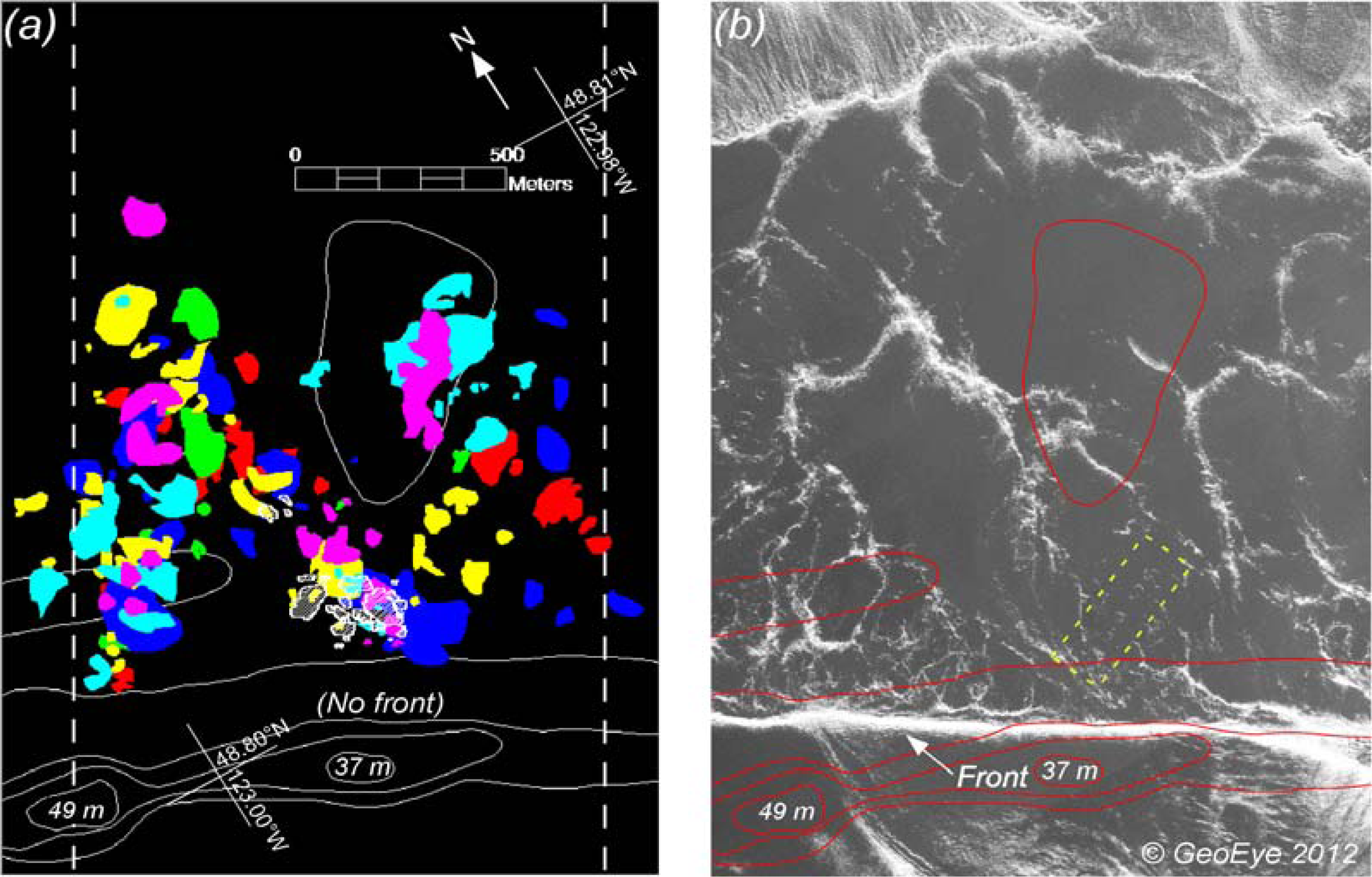
3.4. Spatial Distribution of Boils

A census was made of the boils appearing in the IR data from 1.4 to 2.1 h after ebb. The boils were extracted using the following criteria: (1) A temperature at least 0.5 °C less than the surrounding water; (2) Entire boil perimeter imaged; (3) No connection to an internal wave or a front. The staring-mode data are not included to avoid double counting a boil. All the detected boils lie downstream of the sill and upstream of the tidal convergence front. The results (Figure 11(a)) show a wide range in boil size, but a typical size is in the range of 2,800 to 6,400 m2, or a diameter in the range of about 60 to 90 m. There is no indication that boil locations vary in any systematic way over time. There does, however, appear to be an along-sill modulation in the distribution of the boils: Boils occur closest to the sill crest (∼300 m) and are more numerous downstream of each of two high points on the sill crest; while in the gap between high spots, boils lie ∼600 m from the sill crest. For comparison, Figure 11(b) shows GeoEye panchromatic imagery (1.7 h after ebb) over the same area. (These 0.4-m resolution data show many of the boil-like patterns more clearly than the multispectral data of Figure 4). In this case, the tidal convergence front (visible as a wave-current interaction zone) lies over the sill; nevertheless, boil-like signatures occur in about the same locations and have about the same range in size as the thermal signatures in Figure 11(a). In particular, the series of spatially-periodic, 20-m-diameter boils that was highlighted earlier (Figure 4(c)) seems to trail downstream of one of the high spots on the sill crest, though of course this may simply be a coincidence.

4. Discussion

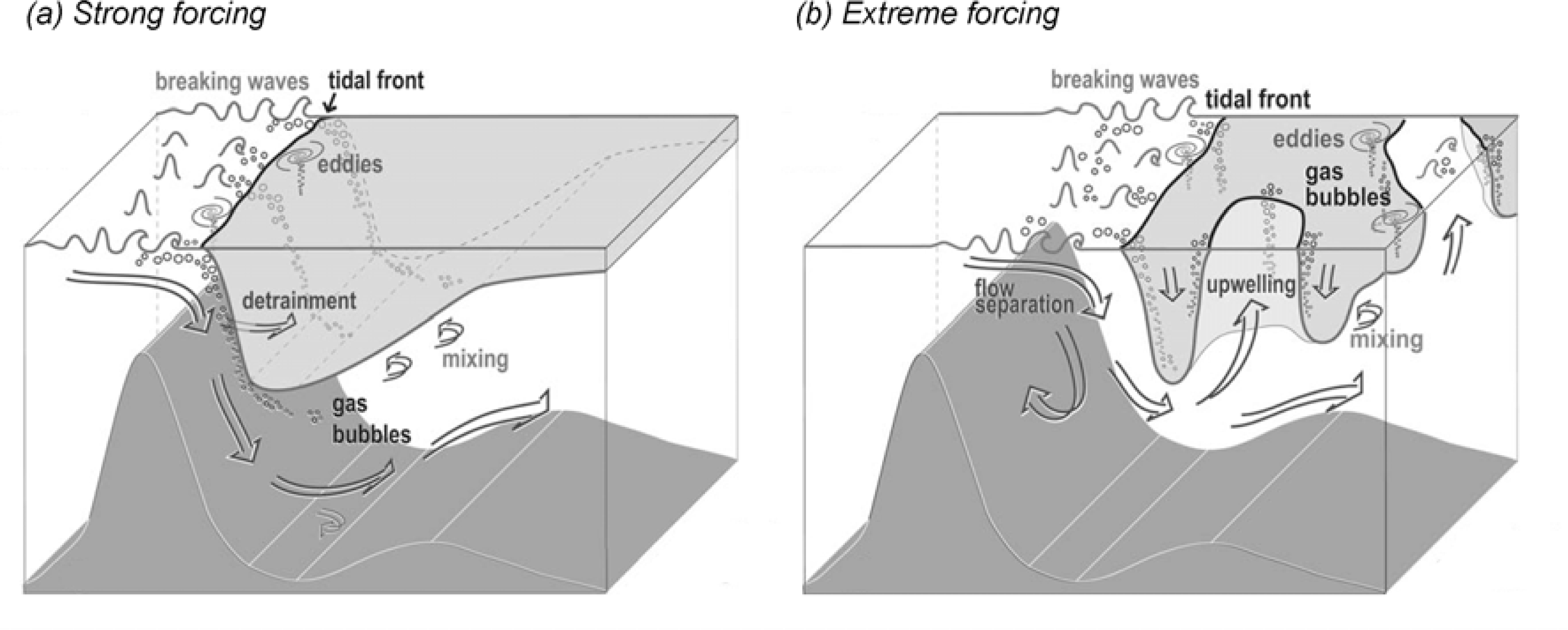
4.1. Comparison with the Expected Flow Response

The image examples capture aspects of the flow response expected during strong forcing (0.5 to 1.5 h after ebb slack) as described in Section 2.1, but there also seem to be some intriguing differences. The GeoEye data (Figure 4), acquired 1.7 h after ebb slack, show a well-defined wave-current interaction zone that has the width (∼50 m) and location (over the sill) expected of the tidal convergence front during strong forcing. However, the occurrence of large-scale surface turbulence (inferred from sunglint patterns) extending 1.6 km from the sill resembles more the extreme forcing stage, when large rings of upwelled water, possibly associated with large-scale overturning cells at the base of the buoyant layer, can be found as far as 2 km from the sill (Section 2.1). In the airborne data (Figure 8), the front is trapped over the sill in early flood, and then moves away from the sill through the end of strong forcing; both effects as expected. Large boils are not seen downstream of the sill early in flood, when the buoyant layer is still present there. Boils emerge only after the front is pushed well downstream from the sill, and then occur in the area between the sill and moving front; the distribution of these boils at a mean time of 1.8 h after ebb slack is indicated in Figure 11(a). This suggests a more direct sill-induced forcing mechanism (examined further below), not previously identified for the study area; and boils produced in this way are an additional source for air-sea gas exchange and vertical mixing.
The satellite and airborne examples thus provide seemingly quite different views of the surface turbulence at a similar stage in the tidal forcing. This difference was unexpected, and it suggests the surface expressions of turbulence may be sensitive to some factor other than tidal stage. Of the environmental variables listed in Table 1 (wind, spring-neap tidal cycle, etc.), it is discharge from the Fraser River that shows the largest difference between the satellite and airborne datasets. Higher river discharge occurred during the satellite acquisitions. Higher discharge would be expected to result in stronger stratification and a thicker plume layer. Signatures of surface turbulence should therefore be less likely in the satellite examples, but this is just the opposite of what the images suggest. It is unclear, therefore, how to account for the different surface expressions. Clearly, analysis of a larger set of images would be helpful in making progress on this question.
An additional aspect of the flow response is the occurrence of internal waves in the buoyant plume layer downstream of the sill (Figure 5). These signatures, which appear to become more coherent with increasing distance from the sill, may arise from vigorous turbulence created in the lee of the sill [29] and in the deep hydraulic jump (Section 2.1).

4.2. Comparison with a “Boil-Surfacing” Model

In this section, an idealized, kinematical model [7] is used to examine the spatial distribution of boils shown in Figure 11(a). The model was developed to account for the location of boils observed in thermal imagery acquired during strong tidal flow (and weak stratification) over a rocky sill in the Snohomish River estuary, WA, USA [7,30,31]; and predictions of boil-surfacing locations were determined from the modeled vertical velocity, the sill depth, and the over-sill velocity [7]. While the sill height and crest depth are of the order of 50 times larger for the Boundary Pass case, the aspect ratio of sill height to total water depth is ∼0.7 in both cases; so we can hypothesize that the dynamics are similar and model applicable.
The model assumes that, to a first approximation, the distance downstream from the sill to a boil’s surfacing point is given by L = U (h/wb), where it is assumed the boil travels downstream at a constant velocity U for a time equal to the sill depth h divided by the boil’s vertical velocity wb, which is also assumed to be constant. To calculate wb, boils are conceptualized as loops of spanwise vorticity (hairpin vortices) generated at the sill crest. Vorticity generated by shear at the sill crest is expected to dominate other effects because of the large sill-to-depth aspect ratio. The resulting boils are hypothesized to self-propagate to the surface via vortex-pair interaction, modeled as a two-dimensional vortex-dipole of a size based on the observed boil diameter. The vortex strength is estimated as U/h. The model is thus able to predict a downstream surfacing location that depends only on the mean boil diameter d and sill depth h. The resulting prediction is L = 8 h2/d.
For the Boundary Pass sill, using h in the range of 37 to 49 m (assuming boils generated from the two high points on the sill) and d∼70 m, the model predicts L in the range of 156 to 274 m. This compares with a value of about 300 m as inferred from the imagery (Figure 11(a)). For boils originating along the sill crest between the two high points, h = 60 m, and the model predicts a value of L = 411 m; the imagery suggests about 600 m. The model seems, therefore, to under-predict the surfacing distance in this application by about 30%. A possible explanation for this is that the model assumes an instantaneous generation of full-sized boils at the sill crest, instead of a smooth growth of the vortex loop as it ascends; thus, the model likely over-predicts wb and consequently under-predicts L.

5. Conclusions

A limited set of visible and thermal imagery, acquired from both satellite and airborne sensors, has been analyzed for evidence of large-scale turbulent structures, or boils, for the particular case of tidal flow over a ∼60-m-deep sill. We can draw the following conclusions:
(1)
Turbulence reaching the sea surface as boils is captured in both thermal and visible imagery.
(2)
Boils appear as relative cold patches where upwelled water displaces an ambient diurnal warm layer. The contrast ranges from about 0.4 °C (under wind speeds of ∼5 m/s) to 1.8 °C (∼2 m/s).
(3)
High-resolution multi-looks, made possible by using a high framing-rate IR camera and by mechanically staring at a particular patch of the sea surface, are able to resolve the growth rate of a boil. A representative large boil grows at a sustained rate of ∼60 m2/s, attaining an areal extent of 3,750 m2 (an equivalent diameter of 70 m) after one minute.
(4)
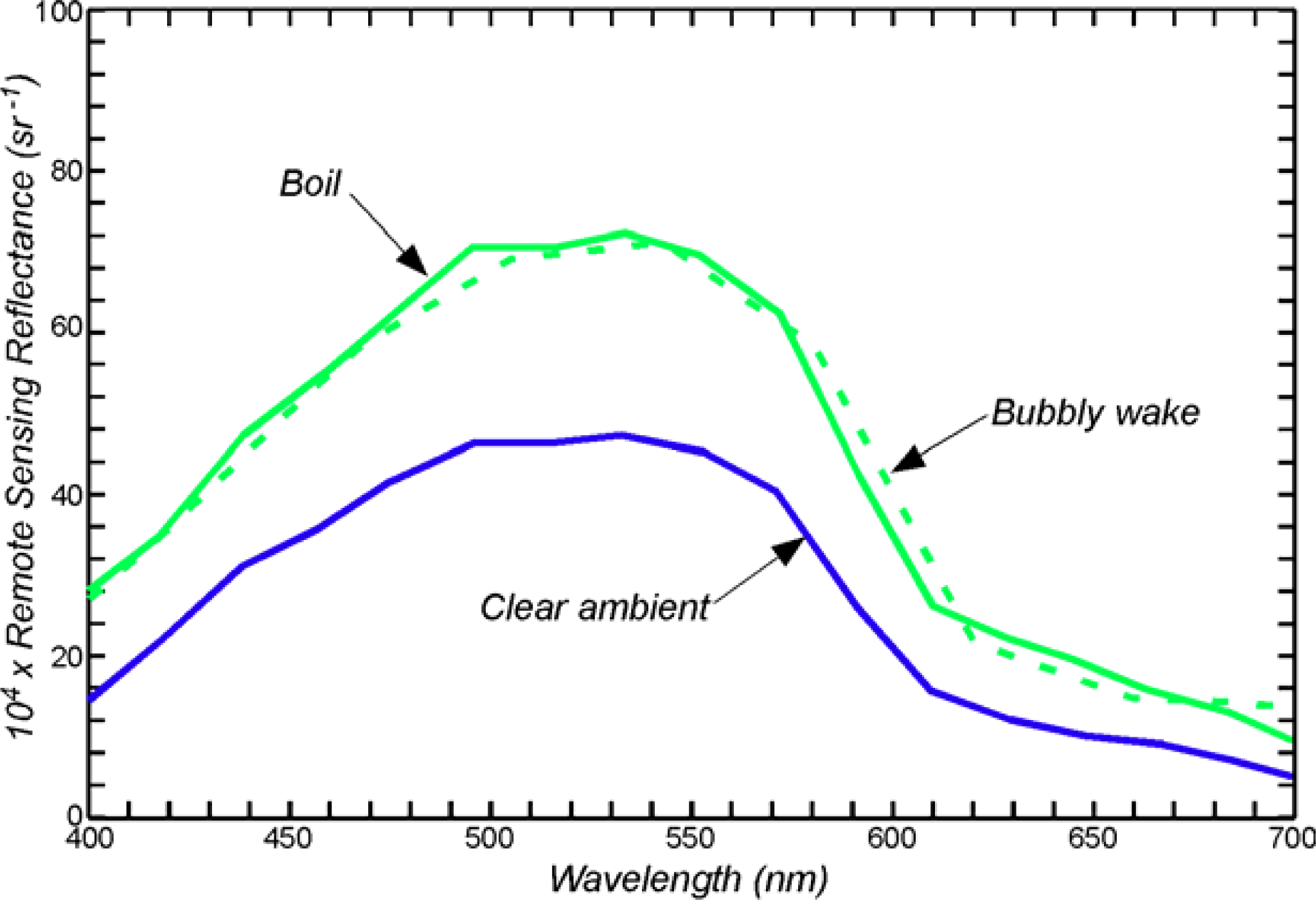
Boils show an enhanced remote sensing reflectance over wavelengths of about 500 to 550 nm. This green-shift is consistent with light backscattering from large submerged “clouds” of air bubbles.
(5)
The data suggest that bubble clouds develop through the re-distribution of locally injected bubbles (from breaking of surface waves) by an underlying volume of turbulent flow.
(6)
Compared with an existing physical framework, unexpected differences in the spatial extent of surface turbulence occur at the same stage in tidal forcing, suggesting a dependence on some other factor, as yet undetermined.
(7)
The occurrence of boils within a few hundred meters downstream of the sill can be tentatively ascribed to vorticity generation at the sill crest. This appears to be a mechanism for vertical mixing not previously identified for the study area, and is an example where in-water measurements coupled with remote sensing data are needed to progress.
(8)
Intense ocean turbulence manifests itself on many spatial scales, and the time scale of large turbulent structures is measured in minutes. Such phenomena are difficult to measure directly, making remote sensing especially useful. Visible and thermal data have provided a starting point for understanding sill-induced turbulence. Synthetic aperture radar imagery, which can measure the surface roughness pattern and the surface current field at high spatial resolution [3234], might be used to quantify the wave-current interaction and kinetic energy associated with the surface turbulence; and multi-look satellite imagery might be used to measure the boil growth rate.

Acknowledgments

This work was made possible through the support of the Office of Naval Research and conducted under Naval Research Laboratory project 72-9201. NRL contribution NRL/JA/7230-13-0057.

Conflict of Interest

The authors declare no conflict of interest.

References

  1. Thorpe, S.A. Recent developments in the study of ocean turbulence. Annu. Rev. Earth Planet. Sci 2004, 32, 91–109. [Google Scholar]
  2. Marmorino, G.O.; Toporkov, J.V.; Smith, G.B.; Sletten, M.A.; Perkovic, D.; Frasier, S.; Judd, K.P. Ocean mixed-layer depth and current variation estimated from imagery of surfactant streaks. IEEE Geosci. Remote Sens. Lett 2007, 4, 364–367. [Google Scholar]
  3. Nimmo Smith, W.A.M.; Thorpe, S.A.; Graham, A. Surface effects of bottom-generated turbulence in a shallow tidal sea. Nature 1999, 400, 251–254. [Google Scholar]
  4. Thorpe, S.A.; Green, J.A.M.; Simpson, J.H.; Osborn, T.R.; Nimmo Smith, W.A.M. Boils and turbulence in a weakly stratified shallow tidal sea. J. Phys. Oceanogr 2008, 38, 1711–1730. [Google Scholar]
  5. Pawlowicz, R. Quantitative visualization of geophysical flows using digital oblique time-lapse imaging. IEEE J. Ocean. Eng 2003, 28, 699–710. [Google Scholar]
  6. Hennings, I.; Herbers, D. Radar imaging mechanism of marine sand waves at very low grazing angle illumination caused by unique hydrodynamic interactions. J. Geophys. Res. 2006, 111. [Google Scholar] [CrossRef] [Green Version]
  7. Chickadel, C.C.; Horner-Devine, A.R.; Talke, S.A.; Jessup, A.T. Vertical boil propagation from a submerged estuarine sill. Geophys. Res. Lett. 2009, 36. [Google Scholar] [CrossRef]
  8. Marmorino, G.O.; Smith, G.B. Thermal remote sensing of estuarine spatial dynamics: Effects of bottom-generated vertical mixing. Estuar. Coast. Shelf Sci 2008, 78, 587–591. [Google Scholar]
  9. Farmer, D.M.; D’Asaro, E.A.; Trevorrow, M.V.; Daikiri, G.T. Three-dimensional structure in a tidal convergence front. Cont. Shelf Res 1995, 15, 1649–1673. [Google Scholar]
  10. Farmer, D.M.; Pawlowicz, R.; Jiang, R. Tilting separation flows: A mechanism for intense vertical mixing in the coastal ocean. Dyn. Atmos. Ocean 2002, 36, 43–58. [Google Scholar]
  11. Chang, M.-H.; Lien, R.-C.; Yang, Y.J.; Tang, T.Y.; Wang, J. A composite view of surface signature and interior properties of nonlinear internal waves: Observations and applications. J. Atmos. Ocean. Technol 2008, 25, 1218–1227. [Google Scholar]
  12. Da Silva, J.C.B.; Magalhaes, J.M.; Batista, M.; Gostiaux, L.; Gerkema, T.; New, A.L. The EUFAR Transnational Access Project A.NEW (Airborne Observations of Nonlinear Evolution of Internal Waves Generated by Internal Tidal Beams). Proceedings of 2012 IEEE International Geoscience and Remote Sensing Symposium (IGARSS), Munich, Germany, 22–27 July 2012; pp. 7601–7604.
  13. Baschek, B.; Farmer, D.M.; Garrett, C. Tidal fronts and their role in air-sea gas exchange. J. Mar. Res 2006, 64, 483–515. [Google Scholar]
  14. Baschek, B. Air-Sea Gas Exchange in Tidal Fronts; Ph.D. Thesis, University of Victoria, Victoria, BC, Canada; 2003; p. 156. [Google Scholar]
  15. Farmer, D.M.; Armi, L. Maximal two-layer exchange over a sill and through the combination of a sill and contraction with barotropic flow. J. Fluid Mech 1986, 164, 53–76. [Google Scholar]
  16. Armi, L.; Farmer, D.M. Stratified flow over topography: Bifurcation fronts and transition to the uncontrolled state. Proc. Roy. Soc. A 2002, 458, 513–538. [Google Scholar]
  17. Largier, J.L. Tidal intrusion fronts. Estuaries 1992, 15, 26–39. [Google Scholar]
  18. Davies, A.M.; Xing, J. On the influence of stratification and tidal forcing upon mixing in sill regions. Ocean Dyn 2007, 57, 431–451. [Google Scholar]
  19. Klymak, J.M.; Gregg, M.C. Tidally generated turbulence over the knight inlet sill. J. Phys. Oceanogr 2004, 34, 1135–1151. [Google Scholar]
  20. Cummins, P.F.; Armi, L. Upstream internal jumps in stratified sill flow: Observations of formation, evolution, and release. J. Phys. Oceangr 2010, 40, 1419–1426. [Google Scholar]
  21. Pawlowicz, R. Observations and linear analysis of sill-generated internal tides and estuarine flow in Haro Strait. J. Geophys. Res 2002, 107, 2156–2202. [Google Scholar]
  22. Gargett, A.E. Generation of internal waves in the Strait of Georgia, British Columbia. Deep-Sea Res 1976, 23, 17–20. [Google Scholar]
  23. Wang, C. Geophysical Observations of Nonlinear Internal Solitary-Like Waves in the Strait of Georgia; Ph.D. Thesis, University British Columbia, Vancouver, BC, Canada; 2009; p. 156. [Google Scholar]
  24. Pawlowicz, R.; Farmer, D.M. Diagnosing vertical mixing in a two-layer exchange flow. J. Geophys. Res 1998, 103, 30695–30711. [Google Scholar]
  25. Hedley, J.D.; Harborne, A.R.; Mumby, P.J. Simple and robust removal of sun glint for mapping shallow-water benthos. Int. J. Remote Sens 2005, 26, 2107–2112. [Google Scholar]
  26. Fairall, C.W.; Bradley, E.F.; Hare, J.E.; Grachev, A.A.; Edson, J.B. Bulk parameterization of air-sea fluxes: Updates and verification for the COARE algorithm. J. Clim 2003, 16, 571–591. [Google Scholar]
  27. Zhang, X.; Lewis, M.; Johnson, B. Influence of bubbles on scattering of light in the ocean. Appl. Opt 1998, 37, 6525–6536. [Google Scholar]
  28. Marmorino, G.O.; Smith, G.B.; Bowles, J.H.; Rhea, W.J. Infrared imagery of ‘breaking’ internal waves. Cont. Shelf Res 2007, 28, 485–490. [Google Scholar]
  29. Aguilar, D.A.; Sutherland, B.R. Internal wave generation from rough topography. Phys. Fluids. 2006, 18. http://dx.doi.org/10.1063/1.2214538.
  30. Talke, S.A.; Horner-Devine, A.R.; Chickadel, C.C. Mixing layer dynamics in separated flow over an estuarine sill with variable stratification. J. Geophys. Res. 2010, 115. [Google Scholar] [CrossRef]
  31. Wang, B.; Giddings, S.N.; Fringer, O.B.; Gross, E.S.; Fong, D.A.; Monismith, S.G. Modeling and understanding turbulent mixing in a macrotidal salt wedge estuary. J. Geophys. Res. 2011, 116. [Google Scholar] [CrossRef]
  32. Lyzenga, D.R.; Johannessen, J.; Marmorino, G. Ocean Currents and Current Boundaries. In SAR Marine User’s Manual; Apel, J., Jackson, C., Eds.; US Department of Commerce: Washington, DC, USA, 2004. [Google Scholar]
  33. Liu, A.K.; Hsu, M.-K. Deriving ocean surface drift using multiple SAR sensors. Remote Sens 2009, 1, 266–277. [Google Scholar]
  34. Romeiser, R.; Suchandt, S.; Runge, H.; Steinbrecher, U.; Grunler, S. First analysis of TerraSAR-X along-track InSAR-derived current fields. IEEE Trans. Geosci. Remote Sens 2010, 48, 820–829. [Google Scholar]
Figure 1. (a) Location of study area (white rectangle); (b) Bathymetry in study area. Blue lines enclose area sampled by aircraft flights. Arrow indicates the direction of the current during flood tide.
Remotesensing 05 03239f1
Figure 2. Sketch of processes active near the sill during strong (a) and extreme (b) flood tidal forcing. View is from the east (From Baschek et al. [13]).
Remotesensing 05 03239f2
Figure 3. LANDSAT Enhanced Thematic Mapper Plus (ETM+) imagery over the area in Figure 1(b). Imagery acquired at 1853 UTC 28 June 2000. (a) Visible imagery; red box highlights two boils; (b) Thermal imagery; temperature scale is approximate. Dashed blue lines as in Figure 1(b). The sill crest only is indicated (dashed yellow curve) as the full set of isobaths masks features of interest. Oppositely-traveling ships appear in the lower left of each panel.
Remotesensing 05 03239f3
Figure 4. GeoEye-1 multispectral imagery from 1934 UTC 14 July 2012. (a) Same spatial extent as in the previous figure. Red curves are isobaths; (b) Enlarged view of sill crest, showing wave-current interaction zone (white band) and a series of small boils (dashed yellow box); (c) Large oval-shaped area with interior boil signatures (arrows).
Remotesensing 05 03239f4
Figure 5. Visible (a) and infrared (IR) (b) data collected at 1939 UT 23 May 2009 at 1,680-m altitude. The scenes are offset by ∼24 s. Red curves are isobaths. Contrast has been stretched to bring out weaker features; sun-glint effects contaminate the right-hand side of the image swath. Black areas lie outside the image swath. Arrow (panel (a)) indicates zone of wave-current interaction. Numbers indicate three water types; see text. Visible (c) and IR (d) data acquired 24 min later (at 2003 UTC) and at 580-m altitude; time offset is ∼9 s. Note change in scale bar. Dashed rectangle highlights a group of boils lying between the sill and front.
Remotesensing 05 03239f5
Figure 6. Spectrum from the interior of the boil signatures in Figure 5(c) compared with spectra from ambient water and from the bubbly wake of a large tanker.
Remotesensing 05 03239f6
Figure 7. (a,b) Enlarged views of the visible and thermal signatures highlighted in Figure 5. Visible boil patches A to E (a) are outlined in red; the same red outlines are repeated in (b). Image acquisition time, t, is measured relative to panel (b). The boils are about 0.4 °C colder than the surrounding water; (c,d) IR data showing the same boils 4 s before and after panel (a). Black dots (e.g., panel (c), lower left corner) are bad camera pixels and should be ignored. Features 1 and 2 illustrate cold imprints that grow over time.
Remotesensing 05 03239f7
Figure 8. (a) Geo-strip from the first pass on 18 May 2009. Across-sill distance (y-axis) is measured relative to the sill crest; (b) Evolution of the across-sill temperature profile, <T(y)>, using data from 15 passes. Brackets indicate averaging in the along-sill (x) direction between the dashed lines shown in (a). Time is measured from ebb slack (0208 UTC). Cloud-contaminated data (final pass) are extrapolated values. Sloping dashed line indicates a frontal translation speed of 0.20 m/s.
Remotesensing 05 03239f8
Figure 9. (a) IR geo-strip from 18 May 2009, 0335 UTC. Rectangle (white dashes) shows the fixed area imaged during data collection in staring mode; (b) A sample frame from the stare imagery, showing a near-nadir view of the sea surface. Area in rectangle (black dashes) is examined in the next figure.
Remotesensing 05 03239f9
Figure 10. Four individual frames (a–d) from the staring-mode imagery of the previous figure. The time interval between successive panels is 10.0 s. Feature A is a boil that grows over the entire image sequence, and is about 1.8 °C colder than the surrounding surface water. Feature B is a boil that gets smaller over time as it subducts beneath the warm stagnant layer. Feature C is an emerging, weakly colder area in the plume water.
Remotesensing 05 03239f10
Figure 11. (a) Boil census, using 1,525-m-altitude airborne data collected on 18 May 2009: red (0335 UTC), green (0344 UTC), blue (0351 UTC), yellow (0359 UTC), cyan (0409 UTC), and magenta (0416 UTC). Area between the dashed vertical lines is common to each pass. Boils from 23 May (extracted from Figure 5(d)) are added as the white crosshatched areas; (b) GeoEye panchromatic imagery (14 July 2012) over the same area.
Remotesensing 05 03239f11
Table 1. Imagery sources and conditions. The number of days since neap tide is shown in parentheses after the date. Hours after ebb slack fall largely within the expected ‘strong forcing’ range of 0.5 to 1.5 h. The current is the predicted speed at maximum flood tide in Boundary Pass. Wind speed (direction) values measured at East Sound, Orcas Island. Right-most column shows weekly Fraser River discharge rates measured at Hope, BC, Canada.
PlatformSensorPixel Size (m)Date (Neap Day)Time (UTC)Hours after Ebb SlackCurrent (m/s)Wind (m/s)Fraser River (m3/s)
LANDSAT ETM+Visible/IR30/6028 June 2000 (+2)18530.61.1∼2 (S)6,940
GeoEye-1Visible1.6; 0.414 July 2012 (+4)19341.71.0<2 (S)8,703
AircraftIR3.5; 7.018 May 2009 (−1)0216–04260.1 to 2.31.0∼2 (S)4,599
AircraftVisible/IR0.3; 0.8/1.3; 3.823 May 2009 (+4)1939–2026−0.2 to 0.61.8∼5 (N)4,895

