Discrimination of Tropical Mangroves at the Species Level with EO-1 Hyperion Data


Abstract
:1. Introduction
2. Materials and Methods
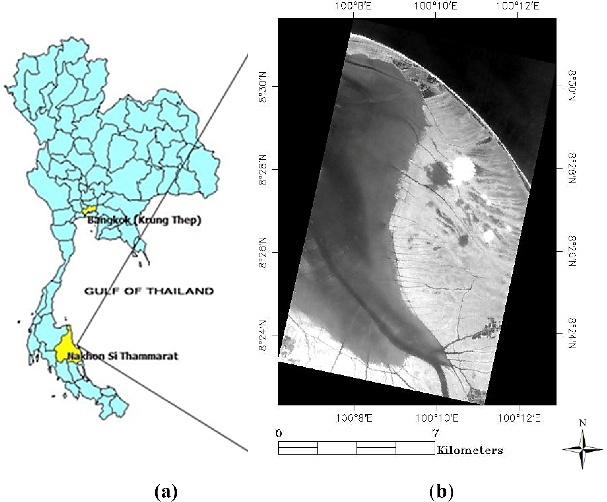
2.1. Study Site
2.2. Image Acquisition and Processing
2.3. Field Data Collection
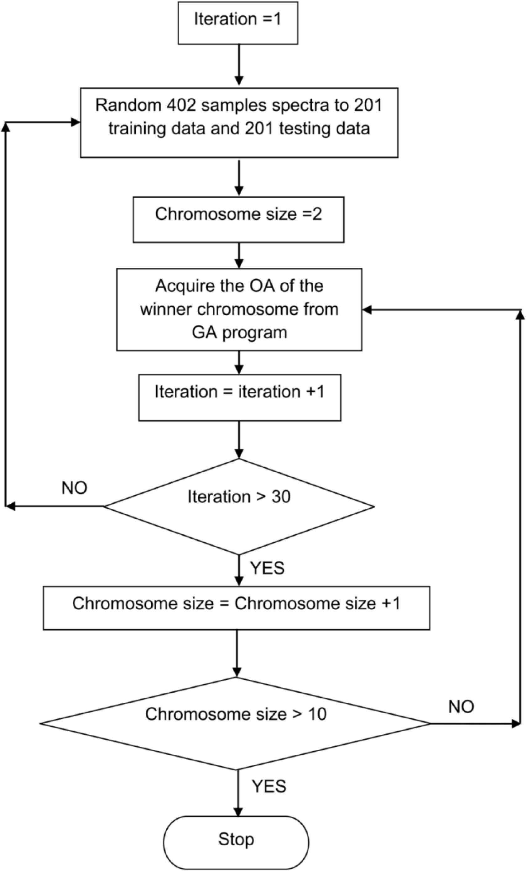
2.4. Genetic Search Algorithm (GA)-Based Band Selection and Classification
2.5. Sequential Forward Selection
2.6. Statistical Test
3. Experiments and Results
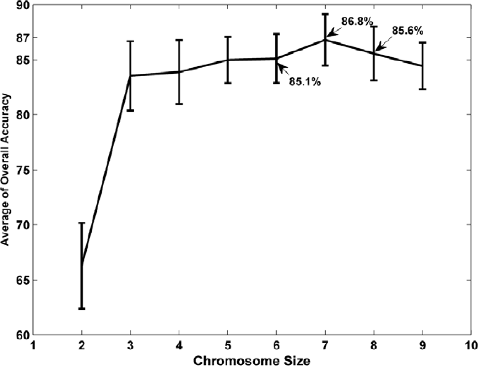
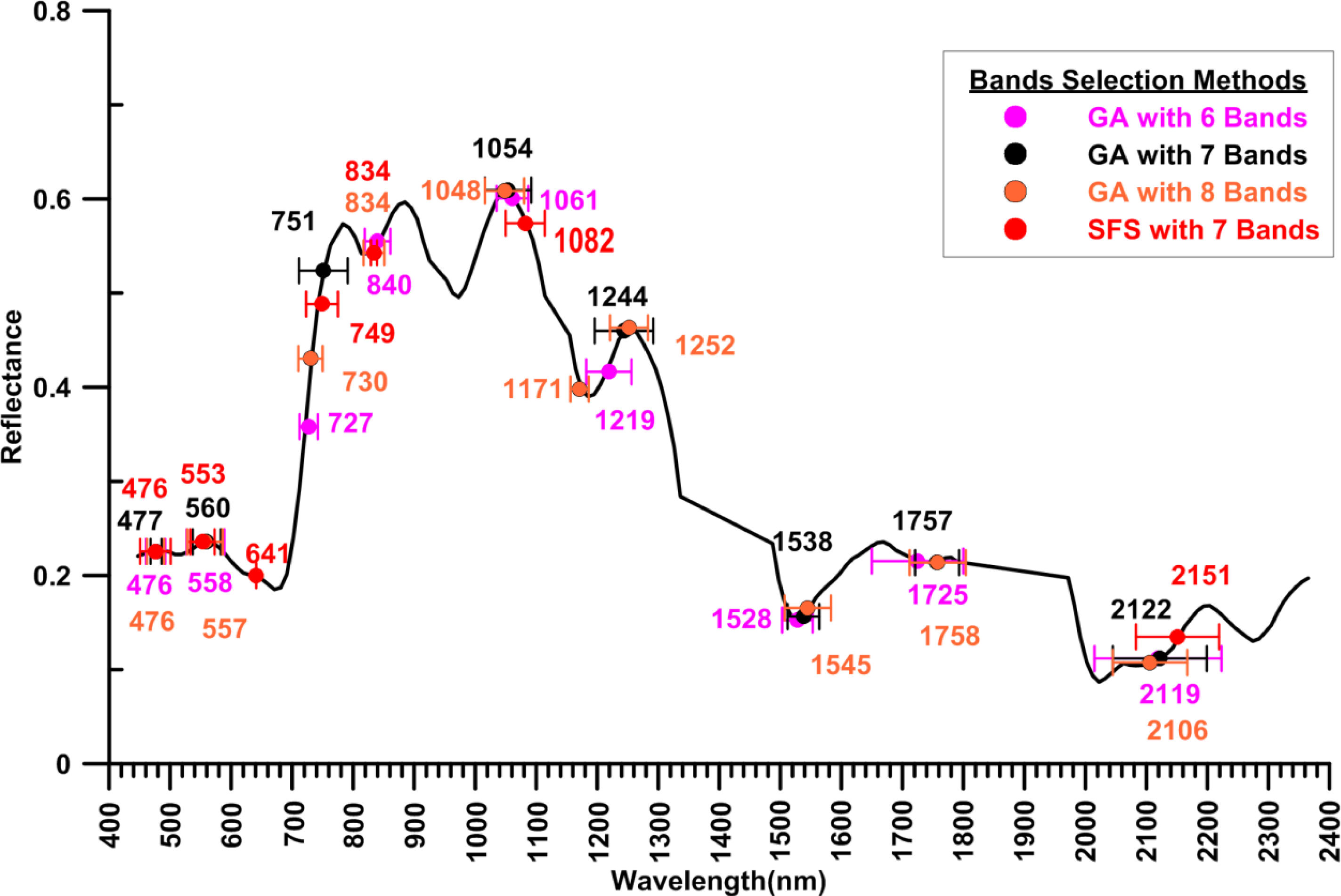
3.1. The Genetic Algorithm (GA) Band Selector
3.2. The Sequential forward Selection
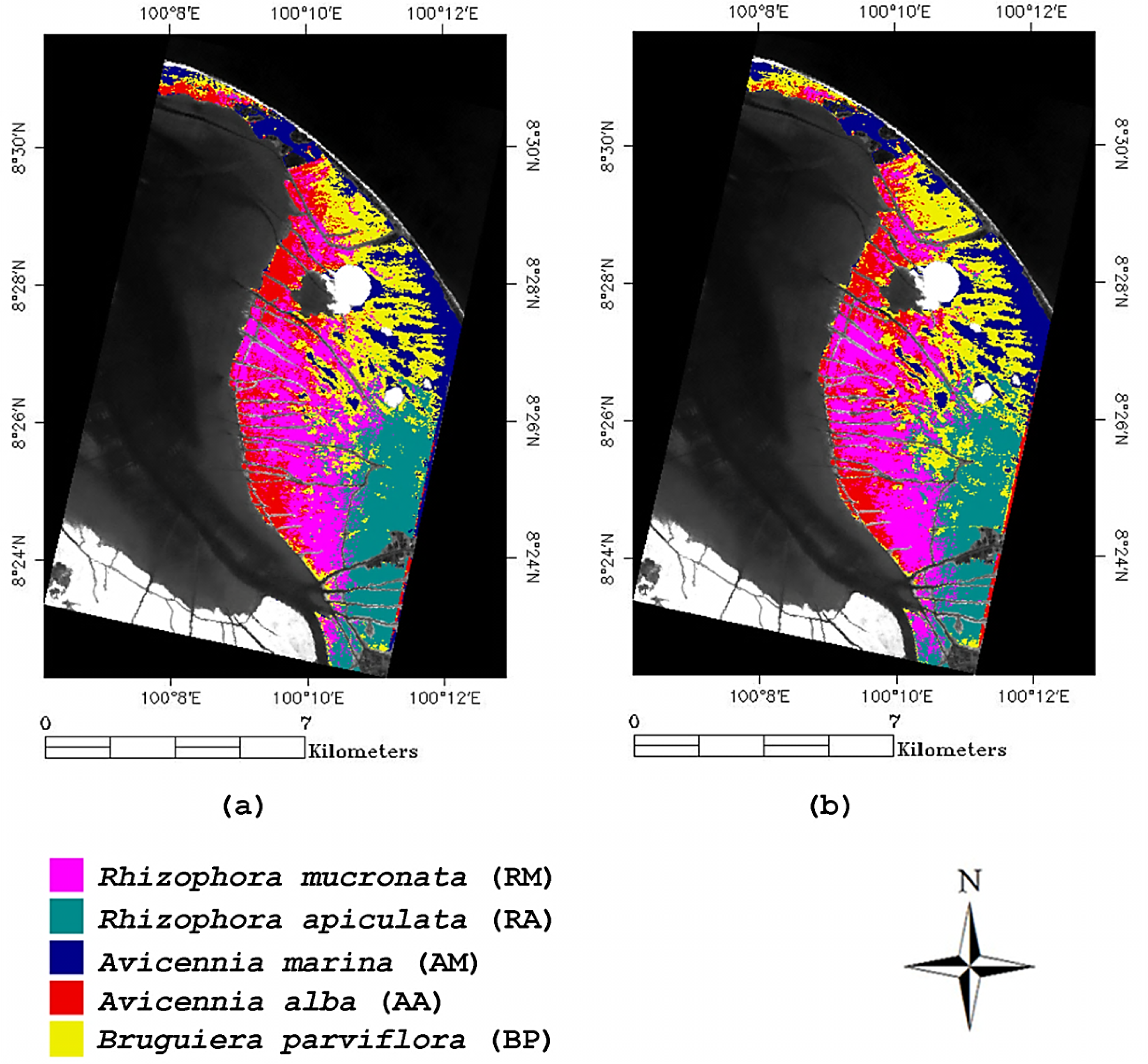
3.3. The Image Classification
4. Discussion
5. Conclusions
Acknowledgments
Conflict of Interest
References
- Food and Agriculture Organization of the United Nations (FAO). The World’s Mangroves 1980–2005; FAO: Rome, Italy, 2007. [Google Scholar]
- Suratman, M.N. Carbon Sequestration Potential of Mangroves in Southeast Asia. In Managing Forest Ecosystems: The Challenge of Climate Change, Managing Forest Ecosystems; Bravo, D.F., Jandl, D.R., LeMay, D.V., von Gadow, P.K., Eds.; Springer: Midtown, NY, USA, 2008; pp. 297–315. [Google Scholar]
- Alongi, D.M. The Energetics of Mangrove Forests, 1st ed; Springer: Midtown, NY, USA, 2009. [Google Scholar]
- Lugo, A.E.; Snedaker, S.C. The ecology of mangroves. Ann. Rev. Ecol. Syst 1974, 5, 39–64. [Google Scholar]
- Adeel, Z.; Pomeroy, R. Assessment and management of mangrove ecosystems in developing countries. Trees-Struct. Funct 2002, 16, 235–238. [Google Scholar]
- Linneweber, V. Mangrove Ecosystems: Function and Management, 1st ed; Springer: New York, NY, USA, 2002. [Google Scholar]
- Barbier, E.; Sathirathai, S. Shrimp Farming and Mangrove Loss in Thailand; Edward Elgar Publishing: Cheltenham, UK, 2004. [Google Scholar]
- McLeod, E.; Salm, R.V. Managing Mangroves for Resilience to Climate Change; World Conservation Union (IUCN): Gland, Switzerland, 2006. [Google Scholar]
- Hogarth, P.J. The Biology of Mangroves and Seagrasses; Oxford University Press: Oxford, UK, 2007. [Google Scholar]
- Zhang, Q.; Middleton, E.M.; Gao, B.C.; Cheng, Y.B. Using EO-1 Hyperion to simulate HyspIRI products for a coniferous forest: The fraction of PAR absorbed by chlorophyll (fAPAR(chl)) and leaf water content (LWC). IEEE Trans. Geosci. Remote Sens 2012, 50, 1844–1852. [Google Scholar]
- Vaiphasa, C.; Boer, W.F.; Skidmore, A.K.; Panitchart, S.; Vaiphasa, T.; Bamrongrugsa, N.; Santitamnont, P. Impact of solid shrimp pond waste materials on mangrove growth and mortality: a case study from Pak Phanang, Thailand. Hydrobiologia 2007, 591, 47–57. [Google Scholar]
- Ellison, A.M.; Farnsworth, E.J. Anthropogenic disturbance of Caribbean mangrove ecosystems: Past impacts, present trends, and future predictions. Biotropica 1996, 549–565. [Google Scholar]
- Farnsworth, E.J.; Ellison, A.M. The global conservation status of mangroves. Ambio 1997, 26, 328–334. [Google Scholar]
- Wang, L.; Sousa, W.P.; Gong, P.; Biging, G.S. Comparison of IKONOS and QuickBird images for mapping mangrove species on the Caribbean coast of Panama. Remote Sens. Environ 2004, 91, 432–440. [Google Scholar]
- Pattanaik, C.; Prasad, S.N. Assessment of aquaculture impact on mangroves of Mahanadi delta (Orissa), East coast of India using remote sensing and GIS. Ocean Coast. Manage 2011, 54, 789–795. [Google Scholar]
- Wilkinson, C.; Salvat, B. Coastal resource degradation in the tropics: Does the tragedy of the commons apply for coral reefs, mangrove forests and seagrass beds. Mar. Pollut. Bull 2012, 64, 1096–1105. [Google Scholar]
- Giesen, W.; Cochran, S.; Scholten, L. Mangrove Guidebook for Southeast Asia; Food and Agriculture Organization of the United Nations, Regional Office for Asia and the Pacific: Bangkok, Thailand, 2006. [Google Scholar]
- Walters, B.B.; Rönnbäck, P.; Kovacs, J.M.; Crona, B.; Hussain, S.A.; Badola, R.; Primavera, J.H.; Barbier, E.; Dahdouh-Guebas, F. Ethnobiology, socio-economics and management of mangrove forests: A review. Aquat. Bot 2008, 89, 220–236. [Google Scholar]
- Song, C.; White, B.L.; Heumann, B.W. Hyperspectral remote sensing of salinity stress on red (Rhizophora mangle) and white (Laguncularia racemosa) mangroves on Galapagos Islands. Remote Sens. Lett 2011, 2, 221–230. [Google Scholar]
- Kairo, J.G.; Kivyatu, B.; Koedam, N. Application of remote sensing and GIS in the management of mangrove forests within and adjacent to Kiunga Marine Protected Area, Lamu, Kenya. Environ. Dev. Sust 2002, 4, 153–166. [Google Scholar]
- Vaiphasa, C.; Skidmore, A.; Deboer, W. A post-classifier for mangrove mapping using ecological data. ISPRS J. Photogramm 2006, 61, 1–10. [Google Scholar]
- Chadwick, J. Integrated LiDAR and IKONOS multispectral imagery for mapping mangrove distribution and physical properties. Int. J. Remote Sens 2011, 32, 6765–6781. [Google Scholar]
- Heumann, B.W. Satellite remote sensing of mangrove forests: Recent advances and future opportunities. Prog. Phys. Geog 2011, 35, 87–108. [Google Scholar]
- Nandy, S.; Kushwaha, S. Study on the utility of IRS 1D LISS-III data and the classification techniques for mapping of Sunderban mangroves. J. Coast. Conserv 2011, 15, 123–137. [Google Scholar]
- Green, E.P.; Mumby, P.J.; Edwards, A.J.; Clark, C.D. Remote Sensing Handbook for Tropical Coastal Management; United Nations Educational, Scientific and Cultural Organization: Paris, France, 2000. [Google Scholar]
- Held, A.; Ticehurst, C.; Lymburner, L.; Williams, N. High resolution mapping of tropical mangrove ecosystems using hyperspectral and radar remote sensing. Int. J. Remote Sens 2003, 24, 2739–2759. [Google Scholar]
- Giri, C.; Zhu, Z.; Tieszen, L.L.; Singh, A.; Gillette, S.; Kelmelis, J.A. Mangrove forest distributions and dynamics (1975–2005) of the tsunami-affected region of Asia. J. Biogeogr 2007, 35, 519–528. [Google Scholar]
- Huang, X.; Zhang, L.; Wang, L. Evaluation of morphological texture features for mangrove forest mapping and species discrimination using multispectral IKONOS imagery. IEEE Geosci. Remote Sens. Lett 2009, 6, 393–397. [Google Scholar]
- Kovacs, J.M.; Liu, Y.; Zhang, C.; Flores-Verdugo, F.; Santiago, F.F. A field based statistical approach for validating a remotely sensed mangrove forest classification scheme. Wetl. Ecol. Manag 2011, 19, 409–421. [Google Scholar]
- Kuenzer, C.; Bluemel, A.; Gebhardt, S.; Quoc, T.V.; Dech, S. Remote sensing of mangrove ecosystems: A review. Remote Sens 2011, 3, 878–928. [Google Scholar]
- Ramsey, E.W.; Jensen, J.R. Remote sensing of mangrove wetlands: Relating canopy spectra to site-specific data. Photogramm. Eng. Remote Sensing 1996, 62, 939–948. [Google Scholar]
- Gao, J. A hybrid method toward accurate mapping of mangroves in a marginal habitat from SPOT multispectral data. Int. J. Remote Sens 1998, 19, 1887–1899. [Google Scholar]
- Green, E.P.; Clark, C.D.; Mumby, P.J.; Edwards, A.J.; Ellis, A.C. Remote sensing techniques for mangrove mapping. Int. J. Remote Sens 1998, 19, 935–956. [Google Scholar]
- Kovacs, J.M.; Wang, J.; Blanco-Correa, M. Mapping disturbances in a mangrove forest using multi-date Landsat TM imagery. Environ. Manage 2001, 27, 763–776. [Google Scholar]
- Sulong, I.; Mohd-Lokman, H.; Mohd-Tarmizi, K.; Ismail, A. Mangrove mapping using Landsat imagery and aerial photographs: Kemaman District, Terengganu, Malaysia. Environ. Dev. Sust 2002, 4, 135–152. [Google Scholar]
- Zharikov, Y.; Skilleter, G.A.; Loneragan, N.R.; Taranto, T.; Cameron, B.E. Mapping and characterising subtropical estuarine landscapes using aerial photography and GIS for potential application in wildlife conservation and management. Biol. Conserv 2005, 125, 87–100. [Google Scholar]
- Dahdouh-Guebas, F.; Verheyden, A.; Kairo, J.G.; Jayatissa, L.P.; Koedam, N. Capacity building in tropical coastal resource monitoring in developing countries: A re-appreciation of the oldest remote sensing method. Int. J. Sust. Dev. World 2006, 13, 62–76. [Google Scholar]
- Everitt, J.H.; Yang, C.; Summy, K.R.; Judd, F.W.; Davis, M.R. Evaluation of color-infrared photography and digital imagery to map black mangrove on the Texas Gulf coast. J. Coast. Res 2007, 231, 230–235. [Google Scholar]
- Conchedda, G.; Durieux, L.; Mayaux, P. An object-based method for mapping and change analysis in mangrove ecosystems. ISPRS J. Photogramm 2008, 63, 578–589. [Google Scholar]
- Bhattarai, B.; Giri, C. Assessment of mangrove forests in the Pacific region using Landsat imagery. J. Appl. Remote Sens 2011, 5, 053509:1–053509:11. [Google Scholar]
- Long, J.B.; Giri, C. Mapping the Philippines’ Mangrove forests using Landsat imagery. Sensors 2011, 11, 2972–2981. [Google Scholar]
- Kovacs, J.M.; Wang, J.; Flores-Verdugo, F. Mapping mangrove leaf area index at the species level using IKONOS and LAI-2000 sensors for the Agua Brava lagoon, Mexican Pacific. Estuar. Coast. Shelf Sci 2005, 62, 377–384. [Google Scholar]
- Gao, J. A comparative study on spatial and spectral resolutions of satellite data in mapping mangrove forests. Int. J. Remote Sens 1999, 20, 2823–2833. [Google Scholar]
- Demuro, M.; Chisholm, L. Assessment of Hyperion for Characterizing Mangrove Communities. Proceedings of the 12th JPL AVIRIS Airborne Earth Science Workshop, Pasadena, CA, USA, 24–28 February 2003.
- Wang, L.; Sousa, W.P.; Gong, P. Integration of object-based and pixel-based classification for mapping mangroves with IKONOS imagery. Int. J. Remote Sens 2004, 25, 5655–5668. [Google Scholar]
- Neukermans, G.; Dahdouh-Guebas, F.; Kairo, J.G.; Koedam, N. Mangrove species and stand mapping in Gazi Bay (Kenya) using Quickbird satellite imagery. J. Spat Sci 2008, 53, 75–86. [Google Scholar]
- Vaiphasa, C.; Ongsomwang, S.; Vaiphasa, T.; Skidmore, A.K. Tropical mangrove species discrimination using hyperspectral data: A laboratory study. Estuar. Coast. Shelf Sci 2005, 65, 371–379. [Google Scholar]
- Van der Meer, F.; de Jong, S.; Bakker, W. Imaging Spectrometry: Basic Analytical Techniques. In Imaging Spectrometry: Basic Principles and Prospective Applications; van der Meer, F., de Jong, Eds.; Springer: Midtown, NY, USA, 2002; pp. 17–61. [Google Scholar]
- Chang, C.I. Hyperspectral Data Exploitation: Theory and Applications, 1st ed; Wiley-Interscience: Hoboken, NJ, USA, 2007. [Google Scholar]
- Campbell, J.B.; Wynne, R.H. Introduction to Remote Sensing, 5th ed; Guilford Press: New York, NY, USA, 2011. [Google Scholar]
- Kamal, M.; Phinn, S. Hyperspectral data for mangrove species mapping: A comparison of pixel-based and object-based approach. Remote Sens 2011, 3, 2222–2242. [Google Scholar]
- Thenkabail, P.S.; Enclona, E.; Ashton, M.; Legg, C.; De Dieu, M. Hyperion, IKONOS, ALI, and ETM plus sensors in the study of African rainforests. Remote Sens. Environ 2004, 90, 23–43. [Google Scholar]
- Thenkabail, P.S.; Smith, R.B.; De Pauw, E. Evaluation of narrowband and broadband vegetation indices for determining optimal hyperspectral wavebands for agricultural crop characterization. Photogram. Eng. Remote Sensing 2002, 68, 607–621. [Google Scholar]
- Goodenough, D.G.; Dyk, A.; Niemann, K.O.; Pearlman, J.S.; Chen, H.; Han, T.; Murdoch, M.; West, C. Processing Hyperion and ALI for forest classification. IEEE Trans. Geosci. Remote Sens 2003, 41, 1321–1331. [Google Scholar]
- Lee, K.S.; Cohen, W.B.; Kennedy, R.E.; Maiersperger, T.K.; Gower, S.T. Hyperspectral versus multispectral data for estimating leaf area index in four different biomes. Remote Sens. Environ 2004, 91, 508–520. [Google Scholar]
- Mutanga, O.; Skidmore, A. Narrow band vegetation indices overcome the saturation problem in biomass estimation. Int. J. Remote Sens 2004, 25, 3999–4014. [Google Scholar]
- Clark, M.L.; Roberts, D.A.; Clark, D.B. Hyperspectral discrimination of tropical rain forest tree species at leaf to crown scales. Remote Sens. Environ 2005, 96, 375–398. [Google Scholar]
- Pu, R.; Yu, Q.; Gong, P.; Biging, G. EO-1 Hyperion, ALI and Landsat 7 ETM+ data comparison for estimating forest crown closure and leaf area index. Int. J. Remote Sens 2005, 26, 457–474. [Google Scholar]
- Rao, N.; Garg, P.; Hosh, S. Estimation and comparison of leaf area index of agricultural crops using IRS LISS-III and EO-1 Hyperion images. Photonirvachak-J. Ind 2006, 34, 69–78. [Google Scholar]
- Vaiphasa, C.; Skidmore, A.K.; de Boer, W.F.; Vaiphasa, T. A hyperspectral band selector for plant species discrimination. ISPRS J. Photogramm 2007, 62, 225–235. [Google Scholar]
- Wang, L.; Sousa, W. Distinguishing mangrove species with laboratory measurements of hyperspectral leaf reflectance. Int. J. Remote Sens 2009, 30, 1267–1281. [Google Scholar]
- Hirano, A.; Madden, M.; Welch, R. Hyperspectral image data for mapping wetland vegetation. Wetlands 2003, 23, 436–448. [Google Scholar]
- Hao, X.; Qu, J.J. Fast and highly accurate calculation of band averaged radiance. Int. J. Remote Sens 2009, 30, 1099–1108. [Google Scholar]
- Hughes, G.F. On mean accuracy of statistical pattern recognizers. IEEE Trans. Inf. Theory 1968, 14, 55. [Google Scholar]
- Zhou, M.D.; Shu, J.O.; Chen, Z.G. Classification of hyperspectral remote sensing image based on genetic algorithm and SVM. Proc. SPIE 2010, 7809. [Google Scholar] [CrossRef]
- Shahshahani, B.M.; Landgrebe, D.A. The effect of unlabeled samples in reducing the small sample size problem and mitigating the Hughes phenomenon. IEEE Trans. Geosci. Remote Sens 1994, 32, 1087–1095. [Google Scholar]
- Sreekala, G.B.; Subodh, S.K. Hyperspectral Data Mining. In Hyperspectral Remote Sensing of Vegetation; Thenkabail, P.S., Lyon, G.J., Huete, A., Eds.; CRC Press: Boca Raton, FL, USA, 2011. [Google Scholar]
- Gomez-Chova, L.; Calpe, J.; Camps-Valls, G.; Martin, J.; Soria, E.; Vila, J.; Alonso-Chorda, L.; Moreno, J. Feature Selection of Hyperspectral Data through Local Correlation and SFFS for Crop Classification. Proceedings of IEEE International Geoscience and Remote Sensing Symposium, Toulouse, France, 21–25 July 2003; pp. 555–557.
- Zhuo, L.; Zheng, J.; Li, X.; Wang, F.; Ai, B.; Qian, J. A Genetic Algorithm Based Wrapper Feature Selection Method for Classification of Hyperspectral Images Using Support Vector Machine. Proceeding of the Geoinformatics 2008 and Joint Conference on GIS and Built Environment: Classification of Remote Sensing Images, Guangzhou, China, 28–29 June 2008; pp. 71471J–71471J.
- Jia, X.; Kuo, B.-C.; Crawford, M.M. Feature mining for hyperspectral image classification. Proc. IEEE 2013, 101, 676–697. [Google Scholar]
- Riedmann, M.; Milton, E.J. Supervised Band Selection for Optimal Use of Data from Airborne Hyperspectral Sensors. Proceeding of the IEEE International Geoscience and Remote Sensing, Toulouse, France, 21–25 July 2003; pp. 1770–1772.
- Ullah, S.; Groen, T.A.; Schlerf, M.; Skidmore, A.K.; Nieuwenhuis, W.; Vaiphasa, C. Using a genetic algorithm as an optimal band selector in the mid and thermal infrared (2.5–14 μm) to discriminate vegetation species. Sensors 2012, 12, 8755–8769. [Google Scholar]
- Li, S.; Wu, H.; Wan, D.; Zhu, J. An effective feature selection method for hyperspectral image classification based on genetic algorithm and support vector machine. Knowl.-Based Syst 2011, 24, 40–48. [Google Scholar]
- Fang, H.; Liang, S.; Kuusk, A. Retrieving leaf area index using a genetic algorithm with a canopy radiative transfer model. Remote Sens. Environ 2003, 85, 257–270. [Google Scholar]
- Teeratanatorn, W. Mangroves of Pak Phanang Bay (in Thai); Royal Forest Department: Bangkok, Thailand, 2000. [Google Scholar]
- Beck, R. EO-1 User Guide-Version 2.3. Satellite Systems Branch; USGS Earth Resources Observation Systems Data Center (EDC): Sioux Falls, SD, USA, 2003. [Google Scholar]
- Datt, B.; McVicar, T.R.; Van Niel, T.G.; Jupp, D.L.; Pearlman, J.S. Preprocessing EO-1 Hyperion hyperspectral data to support the application of agricultural indexes. IEEE Trans. Geosci. Remote Sens 2003, 41, 1246–1259. [Google Scholar]
- Datt, B.; Jupp, D. Hyperion Data Processing Workshop: Hands-on Processing Instruction; CSIRO Earth Observation Centre: Clayton South, VIC, Australia, 2004. [Google Scholar]
- Thenkabail, P.S.; Mariotto, I.; Gumma, M.K.; Middleton, E.M.; Landis, D.R.; Huemmrich, F.K. Selection of hyperspectral narrowbands (HNBs) and composition of hyperspectral twoband vegetation indices (HVIs) for biophysical characterization and discrimination of crop types using field reflectance and Hyperion/EO-1 data. IEEE J. Sel. Top. Appl. Earth Obs 2013, 6, 427–439. [Google Scholar]
- Kaplan, E.D.; Hegarty, C.J. Understanding GPS: Principles and Applications; Artech House Publishers: Norwood, MA, USA, 2006. [Google Scholar]
- Alongi, D.M. Mangrove forests: Resilience; protection from tsunamis; and responses to global climate change. Estuar. Coast. Shelf Sci 2008, 76, 1–13. [Google Scholar]
- Siedlecki, W.; Sklansky, J. A note on genetic algorithms for large-scale feature selection. Pattern Recogn. Lett 1989, 10, 335–347. [Google Scholar]
- Chen, X.; Timothy, A.W.; David, J.C. Integrating visible, near-infrared and short-wave infrared hyperspectral and multispectral thermal imagery for geological mapping at Cuprite, Nevada. Remote Sens. Environ 2007, 110, 344–356. [Google Scholar]
- Cerra, D.; Müller, R.; Reinartz, P. A Classification Algorithm for Hyperspectral Data Based on Synergetics Theory. Proceedings of the ISPRS Annals of the Photogrammetry, Remote Sensing and Spatial Information Sciences, Melbourne, Australia, 25 August–1 September 2012; pp. 71–76.
- Jensen, J.R. Remote Sensing of the Environment: An Earth Resource Perspective, 2nd ed; Prentice Hall Series in Geographic Information Science; Prentice Hall: Upper Saddle River, NJ, USA, 2007. [Google Scholar]
- ENVI User’s Guide. ENVI on-line Software User’s Manual; ITT Visual Information Solutions: Boulder, CO, USA, 2008.
- Richards, J.A. Remote Sensing Digital Image Analysis: An Introduction, 5th ed; Springer: Midtown, NY, USA, 2012. [Google Scholar]
- Somol, P.; Pavel, P. Feature selection toolbox. Pattern Recognit 2002, 12, 2749–2759. [Google Scholar]
- Serpico, S.B.; Moserd, G. Extraction of spectral channels from hyperspectral images for classification purposes. IEEE Trans. Geosci. Remote Sens 2007, 45, 484–494. [Google Scholar]
- Zhang, L.; Zhong, Y.; Huang, B.; Gong, J.; Li, P. Dimensionality reduction based on clonal selection for hyperspectral imagery. IEEE Trans. Geosci. Remote Sens 2007, 45, 4172–4186. [Google Scholar]
- Anderson, J.R.; Hardy, E.H.; Roach, J.T.; Whitmer, R.E. A land use sensor and land cover classification system for use with remote sensing data. Geol. Surv. Prof. Paper 1976, 964, 41. [Google Scholar]
- Tomlinson, P.B. The Botany of Mangroves; Cambridge University Press: Cambridge, UK, 1995. [Google Scholar]
- Williams, P.; Norris, K. Near-Infrared Technology in the Agricultural and Food Industries; American Association of Cereal Chemists: St. Paul, MN, USA, 1987. [Google Scholar]
- Curran, P.J. Remote sensing of foliar chemistry. Remote Sens. Environ. 1989, 30, 271–278. [Google Scholar]
- Elvidge, C.D. Visible and near infrared reflectance characteristics of dry plant materials. Int. J. Remote Sens 1990, 11, 1775–1795. [Google Scholar]
- Kumar, L.; Schmidt, K.; Dury, S.; Skidmore, A. Imaging Spectrometry and Vegetation Science. In Imaging Spectrometry: Basic Principles and Prospective Applications; van der Meer, F., de Jong, S.M., Eds.; Springer: Midtown, NY, USA, 2002; pp. 1–52. [Google Scholar]
- Menon, G.G.; Neelakantan, B. Chlorophyll and light attenuation from the leaves of mangrove species of Kali estuary. Indian J. Mar. Sci 1992, 21, 13–16. [Google Scholar]
- Basak, U.; Das, A.; Das, P. Chlorophylls, carotenoids, proteins and secondary metabolites in leaves of 14 species of mangrove. Bull. Mar. Sci 1996, 58, 654–659. [Google Scholar]
- Das, A.; Parida, A.; Basak, U.; Das, P. Studies on pigments, proteins and photosynthetic rates in some mangroves and mangrove associates from Bhitarkanika, Orissa. Mar. Biol 2002, 141, 415–422. [Google Scholar]
- Yuan, J.; Kaijun, S.; Zheng, N. Vegetation Water Content Estimation Using Hyperion Hyperspectral Data. Proceedings of 2010 18th International Conference on Geoinformatics, Beijing, China, 18–20 June 2010; pp. 1–5.
- Ceccato, P.; Stéphane, F.; Stefano, T.; Stéphane, J.; Jean-Marie, G. Detecting vegetation leaf water content using reflectance in the optical domain. Remote Sens. Environ 2001, 77, 22–33. [Google Scholar]
- Schmidt, K.S.; Skidmore, A.K. Spectral discrimination of vegetation types in a coastal wetland. Remote Sens. Environ 2003, 85, 92–108. [Google Scholar]
- Adam, E.; Mutanga, O. Spectral discrimination of papyrus vegetation (Cyperus papyrus L.) in swamp wetlands using field spectrometry. ISPRS J. Photogramm 2009, 64, 612–620. [Google Scholar]
- Adam, E.M.; Mutanga, O.; Rugege, D.; Ismail, R. Discriminating the papyrus vegetation (Cyperus papyrus L.) and its co-existent species using random forest and hyperspectral data resampled to HYMAP. Int. J. Remote Sens 2012, 33, 552–569. [Google Scholar]
- Goldberg, D.E. Genetic Algorithms in Search, Optimization, and Machine Learning, 1st ed; Addison-Wesley Professional: Reading, MA, USA, 1989. [Google Scholar]
- Mitchell, M. An Introduction to Genetic Algorithms, 3rd ed; MIT Press: Cambridge, MA, USA, 1998. [Google Scholar]
- Fidelis, M.V.; Lopes, H.S.; Freitas, A.A. Discovering Comprehensible Classification Rules with a Genetic Algorithm. Proceedings of the 2000 Congress on Evolutionary Computation, La Jolla, CA, USA, 16–19 July 2000; pp. 805–810.
- Bandyopadhyay, S.; Pal, S.K. Pixel classification using variable string genetic algorithms with chromosome differentiation. IEEE Trans. Geosci. Remote Sens 2001, 39, 303–308. [Google Scholar]


| Mangroves Species | Training Samples | Testing Samples |
|---|---|---|
| Rhizophora mucronata (RM) | 38 | 38 |
| Rhizophora apiculata (RA) | 51 | 51 |
| Avicennia marina (AM) | 44 | 44 |
| Avicennia alba (AA) | 30 | 30 |
| Bruguiera parviflora (BP) | 38 | 38 |
| Total | 201 | 201 |
| (a) | Bands (nm) | OA-Train | OA-Test | Stop Generation | ||||||
|---|---|---|---|---|---|---|---|---|---|---|
| Runs | 1 | 2 | 3 | 4 | 5 | 6 | 7 | |||
| 1 | 488 | 569 | 732 | 983 | 1,034 | 1,245 | 1,790 | 93 | 91 | 41 |
| 2 | 478 | 579 | 732 | 773 | 1,064 | 1,094 | 1,679 | 94 | 86 | 41 |
| 3 | 478 | 579 | 722 | 732 | 1,094 | 1,558 | 2,063 | 93 | 88 | 41 |
| 4 | 569 | 732 | 742 | 824 | 1,023 | 1,760 | 2,063 | 93 | 85 | 41 |
| 5 | 468 | 590 | 732 | 824 | 1,064 | 1,235 | 1,336 | 93 | 88 | 41 |
| 6 | 478 | 569 | 732 | 1,034 | 1,084 | 1,094 | 1,518 | 92 | 89 | 57 |
| 7 | 478 | 579 | 732 | 773 | 1,034 | 1,094 | 1,790 | 92 | 86 | 41 |
| 8 | 468 | 579 | 742 | 824 | 1,064 | 1,235 | 1,760 | 94 | 86 | 51 |
| 9 | 549 | 712 | 732 | 1,034 | 1,235 | 2,073 | 2,083 | 94 | 92 | 41 |
| 10 | 478 | 529 | 539 | 732 | 1,094 | 1,528 | 2,093 | 92 | 88 | 41 |
| 11 | 478 | 579 | 732 | 1,034 | 1,094 | 1,770 | 2,093 | 95 | 88 | 41 |
| 12 | 579 | 732 | 1,034 | 1,235 | 1,518 | 1,548 | 2,032 | 94 | 89 | 38 |
| 13 | 468 | 518 | 579 | 732 | 1,094 | 1,710 | 1,790 | 91 | 90 | 40 |
| 14 | 468 | 488 | 559 | 732 | 1,034 | 1,094 | 2,083 | 93 | 87 | 41 |
| 15 | 478 | 732 | 1,044 | 1,165 | 1,225 | 1,548 | 1,588 | 96 | 84 | 41 |
| 16 | 478 | 488 | 712 | 732 | 1,034 | 1,094 | 2,184 | 96 | 87 | 53 |
| 17 | 478 | 569 | 732 | 1,044 | 1,094 | 2,093 | 2,234 | 95 | 88 | 56 |
| 18 | 518 | 569 | 732 | 1,034 | 1,054 | 1,276 | 1,296 | 93 | 86 | 41 |
| 19 | 579 | 712 | 732 | 834 | 1,044 | 2,184 | 2,214 | 92 | 86 | 43 |
| 20 | 529 | 579 | 712 | 732 | 824 | 1,054 | 1,760 | 92 | 86 | 41 |
| 21 | 478 | 579 | 712 | 773 | 915 | 1,064 | 1,094 | 92 | 83 | 41 |
| 22 | 539 | 569 | 712 | 732 | 1,044 | 1,235 | 1,548 | 94 | 90 | 41 |
| 23 | 457 | 478 | 712 | 732 | 773 | 854 | 1,094 | 95 | 86 | 41 |
| 24 | 478 | 518 | 732 | 824 | 1,225 | 1,336 | 2,073 | 93 | 84 | 41 |
| 25 | 478 | 712 | 732 | 793 | 1,266 | 1,498 | 1,528 | 93 | 83 | 41 |
| 26 | 559 | 732 | 824 | 1,044 | 1,165 | 1,760 | 2,093 | 91 | 88 | 41 |
| 27 | 457 | 569 | 722 | 732 | 742 | 773 | 1,034 | 92 | 87 | 41 |
| 28 | 488 | 529 | 712 | 773 | 824 | 844 | 1,235 | 94 | 82 | 48 |
| 29 | 498 | 518 | 712 | 732 | 1,034 | 1,094 | 2,305 | 93 | 86 | 41 |
| 30 | 579 | 742 | 983 | 1,034 | 1,054 | 1,195 | 2,083 | 93 | 88 | 54 |
| (b) | Bands (nm) | OA | Kappa | ||||||
|---|---|---|---|---|---|---|---|---|---|
| Runs | 1 | 2 | 3 | 4 | 5 | 6 | 7 | ||
| 1 | 468 | 539 | 641 | 834 | 1,094 | 1,972 | 2,103 | 67 | 0.58 |
| 2 | 559 | 590 | 641 | 773 | 1,094 | 2,032 | 2,163 | 78 | 0.72 |
| 3 | 447 | 529 | 539 | 579 | 824 | 834 | 2,163 | 74 | 0.68 |
| 4 | 498 | 529 | 569 | 641 | 702 | 773 | 1,094 | 84 | 0.80 |
| 5 | 569 | 579 | 702 | 732 | 834 | 844 | 1,094 | 85 | 0.81 |
| 6 | 498 | 529 | 539 | 579 | 641 | 773 | 2,204 | 80 | 0.74 |
| 7 | 447 | 539 | 569 | 732 | 834 | 1,094 | 2,204 | 83 | 0.79 |
| 8 | 498 | 529 | 569 | 732 | 834 | 1,094 | 2,163 | 86 | 0.82 |
| 9 | 498 | 539 | 569 | 732 | 773 | 1,034 | 1,094 | 87 | 0.83 |
| 10 | 447 | 498 | 569 | 732 | 773 | 1,094 | 2,163 | 85 | 0.81 |
| 11 | 498 | 529 | 569 | 732 | 773 | 1,094 | 2,032 | 86 | 0.82 |
| 12 | 498 | 529 | 569 | 732 | 773 | 1,094 | 2,163 | 86 | 0.82 |
| 13 | 447 | 498 | 539 | 569 | 773 | 1,094 | 2,163 | 83 | 0.79 |
| 14 | 498 | 529 | 569 | 732 | 773 | 963 | 1,034 | 81 | 0.76 |
| 15 | 498 | 529 | 569 | 641 | 773 | 1,094 | 2,204 | 83 | 0.78 |
| 16 | 498 | 539 | 569 | 702 | 732 | 834 | 1,094 | 84 | 0.80 |
| 17 | 529 | 569 | 641 | 702 | 732 | 773 | 2,204 | 81 | 0.76 |
| 18 | 539 | 569 | 641 | 732 | 773 | 1,094 | 2,204 | 83 | 0.79 |
| 19 | 447 | 529 | 539 | 569 | 641 | 773 | 2,163 | 76 | 0.69 |
| 20 | 447 | 529 | 569 | 641 | 732 | 773 | 2,204 | 82 | 0.77 |
| 21 | 447 | 498 | 529 | 569 | 732 | 834 | 1,094 | 84 | 0.79 |
| 22 | 529 | 590 | 641 | 732 | 773 | 1,094 | 2,204 | 86 | 0.82 |
| 23 | 498 | 569 | 702 | 732 | 773 | 1,094 | 2,204 | 86 | 0.82 |
| 24 | 447 | 539 | 569 | 641 | 732 | 773 | 1,023 | 81 | 0.76 |
| 25 | 447 | 529 | 539 | 569 | 641 | 773 | 1,094 | 84 | 0.79 |
| 26 | 498 | 529 | 569 | 732 | 773 | 1,094 | 2,163 | 87 | 0.84 |
| 27 | 447 | 498 | 539 | 641 | 732 | 834 | 1,094 | 84 | 0.80 |
| 28 | 447 | 539 | 569 | 641 | 773 | 834 | 2,163 | 71 | 0.64 |
| 29 | 498 | 529 | 569 | 641 | 773 | 1,094 | 2,032 | 84 | 0.79 |
| 30 | 498 | 559 | 579 | 641 | 773 | 1,094 | 2,204 | 85 | 0.81 |
| (a) | ||||||||
| Class | RM | RA | AM | AA | BP | Total | Producer’s Accuracy | User’s Accuracy |
| RM | 34 | 3 | 0 | 1 | 0 | 38 | 89 | 89 |
| RA | 3 | 43 | 0 | 0 | 1 | 47 | 84 | 91 |
| AM | 0 | 0 | 43 | 0 | 0 | 43 | 98 | 100 |
| AA | 1 | 3 | 1 | 29 | 1 | 35 | 97 | 83 |
| BP | 0 | 2 | 0 | 0 | 36 | 38 | 95 | 95 |
| Total | 38 | 51 | 44 | 30 | 38 | 201 | ||
| (b) | ||||||||
| Class | RM | RA | AM | AA | BP | Total | Producer’s Accuracy | User’s Accuracy |
| RM | 26 | 8 | 0 | 0 | 0 | 34 | 68 | 76 |
| RA | 8 | 42 | 0 | 1 | 1 | 52 | 82 | 80 |
| AM | 0 | 0 | 44 | 0 | 1 | 45 | 100 | 97 |
| AA | 4 | 0 | 0 | 27 | 0 | 31 | 90 | 87 |
| BP | 0 | 1 | 0 | 2 | 36 | 39 | 94 | 92 |
| Total | 38 | 51 | 44 | 30 | 38 | 201 | ||
| (c) | ||||||||
| Class | RM | RA | AM | AA | BP | Total | Producer’s Accuracy | User’s Accuracy |
| RM | 23 | 4 | 2 | 0 | 1 | 30 | 61 | 77 |
| RA | 13 | 44 | 0 | 0 | 0 | 57 | 86 | 77 |
| AM | 0 | 0 | 42 | 0 | 2 | 44 | 95 | 95 |
| AA | 2 | 2 | 0 | 29 | 0 | 33 | 97 | 88 |
| BP | 0 | 1 | 0 | 1 | 35 | 37 | 92 | 95 |
| Total | 38 | 51 | 44 | 30 | 38 | 201 | ||
© 2013 by the authors; licensee MDPI, Basel, Switzerland This article is an open access article distributed under the terms and conditions of the Creative Commons Attribution license (http://creativecommons.org/licenses/by/3.0/).
Share and Cite
Koedsin, W.; Vaiphasa, C. Discrimination of Tropical Mangroves at the Species Level with EO-1 Hyperion Data. Remote Sens. 2013, 5, 3562-3582. https://doi.org/10.3390/rs5073562
Koedsin W, Vaiphasa C. Discrimination of Tropical Mangroves at the Species Level with EO-1 Hyperion Data. Remote Sensing. 2013; 5(7):3562-3582. https://doi.org/10.3390/rs5073562
Chicago/Turabian StyleKoedsin, Werapong, and Chaichoke Vaiphasa. 2013. "Discrimination of Tropical Mangroves at the Species Level with EO-1 Hyperion Data" Remote Sensing 5, no. 7: 3562-3582. https://doi.org/10.3390/rs5073562