Article

Pasture Monitoring Using SAR with COSMO-SkyMed, ENVISAT ASAR, and ALOS PALSAR in Otway, Australia

School of Civil and Environmental Engineering, the University of New South Wales, Sydney, NSW 2052, Australia
*
Author to whom correspondence should be addressed.
Remote Sens. 2013, 5(7), 3611-3636; https://doi.org/10.3390/rs5073611
Submission received: 30 May 2013 / Revised: 17 July 2013 / Accepted: 17 July 2013 / Published: 22 July 2013

Abstract

:
Because of all-weather working ability, sensitivity to biomass and moisture, and high spatial resolution, Synthetic aperture radar (SAR) satellite images can perfectly complement optical images for pasture monitoring. This paper aims to examine the potential of the integration of COnstellation of small Satellites for the Mediterranean basin Observasion (COSMO-SkyMed), Environmental Satellite Advanced Synthetic Aperture Radar (ENVISAT ASAR), and Advanced Land Observing Satellite Phased Array type L-band Synthetic Aperture Radar (ALOS PALSAR) radar signals at horizontally emitted and received polarization (HH) for pasture monitoring at the paddock scale in order to guide farmers for better management. The pasture site is selected, in Otway, Victoria, Australia. The biomass, water content of grass, and soil moisture over this site were analyzed with these three bands of SAR images, through linear relationship between SAR backscattering coefficient, and vegetation indices Normalized Differential Vegetation Index (NDVI), Normalized Difference Water Index (NDWI), Enhanced Vegetation Index (EVI)), together with soil moisture index (MI). NDVI, NDWI, and MI are considered as proxy of pasture biomass, plant water content, and soil moisture, respectively, and computed from optical images and climate data. SAR backscattering coefficient and vegetation indices are computed within a grass zone, defined by classification with MODIS data. The grass condition and grazing activities for specific paddocks are detectable, based on SAR backscatter, with all three wavelengths datasets. Both temporal and spatial analysis results show that the X-band SAR has the highest correlation to the vegetation indices. However, its accuracy can be affected by wet weather due to its sensitivity to the water on leaves. The C-band HH backscattering coefficient showed moderate reliability to evaluate biomass and water content of grass, with limited influence from rainfall in the dry season. The L-band SAR is the less accurate one for grass biomass measurement due to stronger penetration.

1. Introduction

Pastures represent one type of managed landscape units in the terrestrial system. Pastures are essential contributors to the productivity and biodiversity of the biosphere, supporting domesticated livestock as a key component of ecosystem. Good pasture management and optimal feed use are, therefore, important for sustainability of the ecosystem as well as prosperity of pasture. Improved utilization of pastures can be achieved by implementation of intensive rotational grazing mechanisms. Rotational grazing involves controlled movement of herds, from paddock to paddock, according to the amount of available biomass or feed in both the current and the destination paddock. A paddock is a small field of grassland, normally fenced and separated by farmers for keeping sheep or cattle. In these intensive grazing systems, pasture biomass must be regularly estimated at the paddock scale for better grazing rotation. Paddocks with higher biomass may be used to lengthen the grazing interval while paddocks with lower biomass should be allowed more time to grow to the desired mass. Traditional biomass estimates are done by using a rising plate meter to measure grass height and convert to biomass. The process is time consuming, requires field work skill, and is limited to single transect [1].
The space borne remote sensing images are used for measuring and mapping pasture biomass, because of its capacity of providing repeated observations over a large area. Using multispectral optical images, the seasonal pattern of Normalized Differential Vegetation Index (NDVI) has been used for classification of grassland in North America [2] and Eastern Australia [3]. NDVI has been widely used for estimation of grass biomass [4,5]. The “Pastures from Space” project in Western Australia was aimed to provide biomass information from Moderate Resolution Imaging Spectroradiometer (MODIS) data at the paddock scale [6,7]. However, with the 250 m spatial resolution, it cannot provide biomass information for a whole paddock because of unavailable mixed pixels in between paddocks. Various vegetation indices from 30 m resolution Landsat Thematic Mapper (TM) imagery were used for pasture biomass in Central Italy, and it was found that NDVI provided the most accurate estimation for grass biomass [5]. Landsat TM images were employed to estimate pasture biomass at the paddock scale in Western Australia [8], but it is difficult to deliver high temporal resolution (weekly and/or daily) information because with low repeating frequency (16 days), and cloud interference, it will be up to one month without data. Therefore, high-resolution Synthetic aperture radar (SAR) and Landsat TM could be combined for pasture biomass estimation in order to deliver information with high temporal and spatial resolution. SAR data was combined with NDVI for cereal yield modeling in Finland, only for validation, while the study was focused on using NDVI for yield estimation [9].
NDVI is able to stand for biomass, but cannot describe plant water content accurately. The Normalized Difference Water Index (NDWI) is commonly used as an accurate estimate of plant water content [10]. It has been successfully applied to the remote detection of plant water content for grasslands [11]. Enhanced Vegetation Index (EVI) is an “optimized” index designed to enhance the vegetation signal with improved sensitivity in high biomass region, and it is also an improvement of vegetation monitoring through de-coupling of the canopy background signal and a reduction in atmospheric influences [12,13]. While the NDVI is chlorophyll sensitive, the EVI is more responsive to canopy structural variations, including canopy type, plant physiognomy, and canopy architecture. While these optically based studies show promise for pasture monitoring, they are always hampered by cloud conditions and night. This has led to our interest in integrating radar techniques with the multispectral optical indices for pasture monitoring research.
SAR work with microwaves that can penetrate clouds [14]. Furthermore, a change in moisture content of grass and soil generally provokes a significant change in their electric properties which influence the absorption, transmission, and reflection of microwave energy. Thus, apart from the height of grass, the moisture content of grass and soil will influence the reflected energy from grassland [15,16]. Nevertheless, investigations on grasslands by using SAR technology are not as intensive as on crops and forests. There are generally two methods for retrieval of vegetation parameters: the physical scattering model and empirical model. As far as the physical scattering model is concerned, in the past 30 years, direct scattering models have been developed from water cloud [17] and the Oh model [18] to the radiative transfer model [19,20], and the complicated Integral Equation Method (IEM) [21,22]. However, the mathematical formulation of these models is complicated and makes a direct inversion difficult. Then, on the basis of statistical approaches, such as neural network, some promising results were obtained for inversion of soil moisture [23] and plant water content of crops [24]. It needs to be pointed out that, for scattering models, a complete ground truth database, concurrent to radar acquisitions, need to be built up. Moreover, the spatial variability of the soil and vegetation properties, from one locality to another, complicates the application of the modeling. Thus, it is more suitable for using these models’ parameters for larger areas than a paddock. A paddock is small and its vegetation variation is significantly affected by human activities such as grazing and mowing.
When it comes to empirical modeling, very few researches were directly carried out for grass biomass or water content. A correlation was found between the C-band (ERS) VV backscatter density and grass height, and due to the fact that the plant height correlates with the biomass, the grass biomass can be estimated indirectly [25]. ERS VV backscatter was sensitive to biomass of totora reeds and bofedal grasslands in wetland, and this sensitivity was highly related to the underlying water surface or water-saturated soil [16]. The other studies involving grass focused on classification, where grass was one of the several ground cover classes. For example, the potential of airborne SAR has been explored for grassland classification, using relationships between mean herbage height and C- and L-backscatter in grassland in New South Wales, Australia [3]. The results suggest that combined imagery from C-and L-band satellite-borne SAR sensors have potential for current application in grassland monitoring. To assess the capability of satellite C-band and L-band for pasture monitoring, Environmental Satellite Advanced Synthetic Aperture Radar (ENVISAT ASAR) and Advanced Land Observing Satellite Phased Array type L-band Synthetic Aperture Radar (ALOS PALSAR) will be used in this study in Otway, Australia.
The use of X-band is expected to be appropriate for pasture biomass, since the scale of pasture and the wavelength is comparable [1,26,27]. However, very limited studies regarding pasture were carried out, and few consistent results were found. For example, in pasture areas in New Zealand, TerraSAR-X HH+HV backscatter performed the best among all polarization combinations, with a residual standard error of 317 kg/ha [28]. In contrast, when using TerraSAR-X dual polarization (HH/VV) for pastures in Queensland, Australia, R2 of relationship between SAR backscatter and individual variables (biomass, soil moisture, and roughness) was too low, indicating that the vegetation, as well as the soil surface, contribute to the net backscatter [29]. In a study of nature conservation sites in the Alpine region [30], the data of COnstellation of small Satellites for the Mediterranean basin Observation (COSMO-SkyMed) was used, and it was found that the potential of VV backscatter to detect grazing or mowing activities was undermined by rainfall events, which made backscatter signal increase sharply. The COSMO-SkyMed (CSK) system, with its four identical constellation satellites, is capable of acquiring frequent images at a high spatial resolution of one meter, twice a day. Thus, the temporal and spatial variation of SAR backscattering with grass growth is worth investigation using CSK data. Moreover, to our knowledge, pasture monitoring using CSK X-band time series images at HH polarization has not been done. Therefore, HH polarization of CSK, together with ENVISAT ASAR and ALOS PALSAR, will be a good opportunity to offer to the community of pasture biomass research.
The combination of SAR images at three different frequencies and the large amounts of SAR images are an added value of this study of pasture monitoring. However, it is very difficult and costly to collect a large amount of ground data corresponding to SAR at each paddock, on 77 dates, for modeling between field measurements and SAR signal. To lower the costs, the research in this paper was conducted by relating SAR signal to spectral vegetation indices (NDVI, NDWI, and EVI) as well as soil moisture index (MI), to study how SAR backscatter changes following pasture properties. NDVI and NDWI, obtained from MODIS and Landsat TM, are substitutes of biomass and plant water content, respectively, while MI is a proxy of soil moisture. Unlike the traditional regression model between ground data and SAR signal, this method proposed herein is a cost-effective and original way to investigate the potential of SAR data for pasture biomass monitoring.
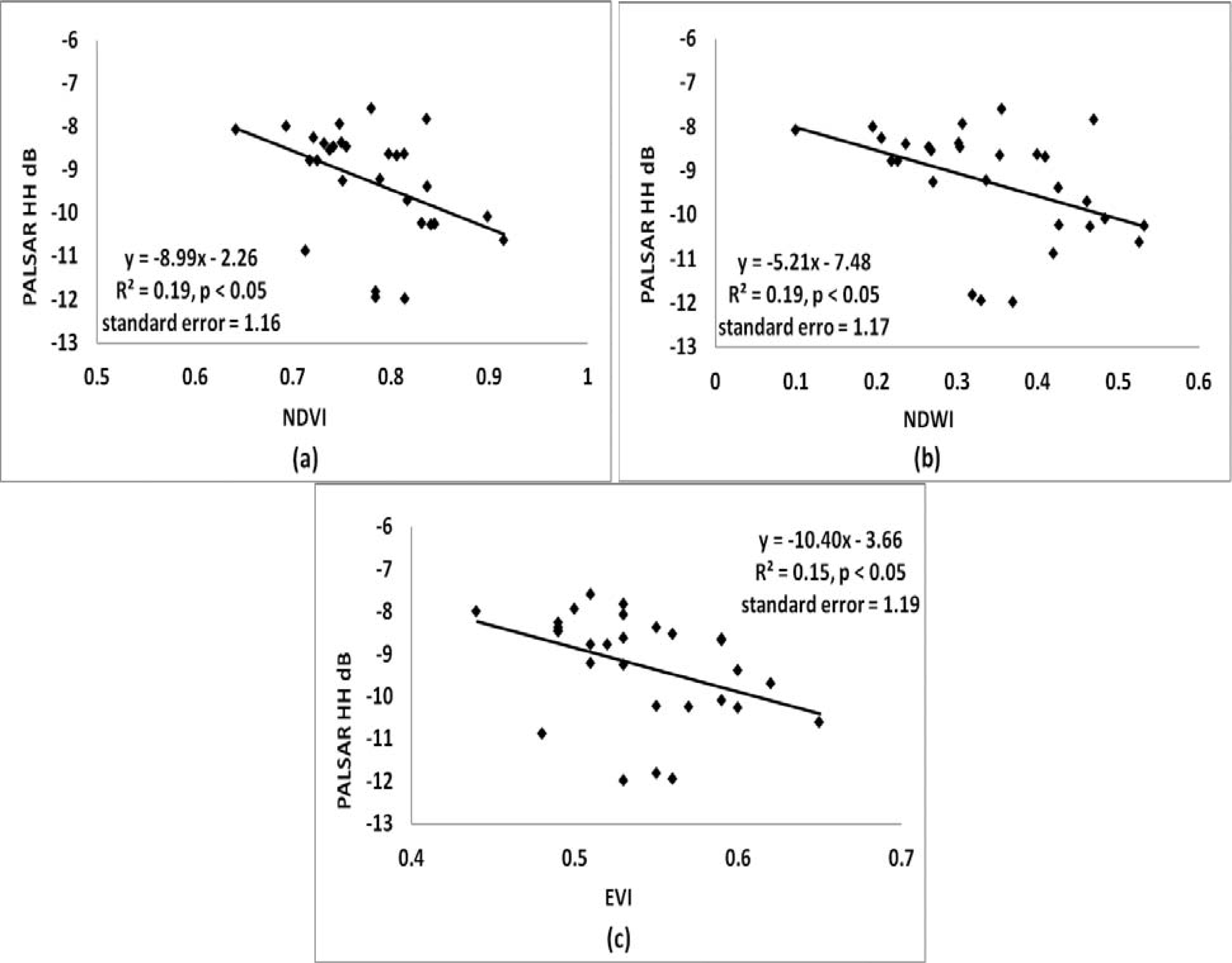
The first objective of this research is to observe the variability of X-, C-, and L-band SAR signals corresponding to grass growth and grazing activities in the whole study area, with the assistance of MI and MODIS NDVI and NDWI. The second objective is to investigate the potential of using SAR to estimate paddock-by-paddock variations of pasture biomass and plant water content on certain dates, with the correlation of Landsat TM vegetation indices NDVI, NDWI, and EVI. The Landsat TM images are generally sparser due to low revisit frequency (16 days per cycle) and clouds and, thus, cannot be used for time series analysis. However, its higher spatial resolution of 30 m makes it capable of doing spatial analysis at the paddock scale on limited imaging dates.

2. Methodology

The objective of this study is to investigate the capability of CSK, ENVISAT ASAR, and ALOS PALSAR at HH polarization for pasture monitoring, thereafter to integrate SAR with optical images to shorten the revisit interval to approach near real-time observation of pastures at the paddock scale. To achieve this, the relationship of SAR backscattering coefficient was performed against optical vegetation indices (NDVI, NDWI), as well as soil moisture index (MI), which were obtained simultaneously to SAR data and used to assist our understanding of the potential of SAR for pastures.
As discussed in Section 1, for pasture monitoring at the paddock scale, the Landsat TM dataset is far better than MODIS’ due to the higher spatial resolution. On the other hand, considering the long revisit interval of the Landsat satellite, using frequent MODIS imagery for temporal analysis is essential. Additionally, annual grass growth pattern of a large region can be obtained from MODIS and used as a reference to benchmark the individual paddocks. Therefore, classification with MODIS images is required to extract grass zones from the whole study area, before further correlation analysis. The following paragraph describes the three main steps of data analysis.
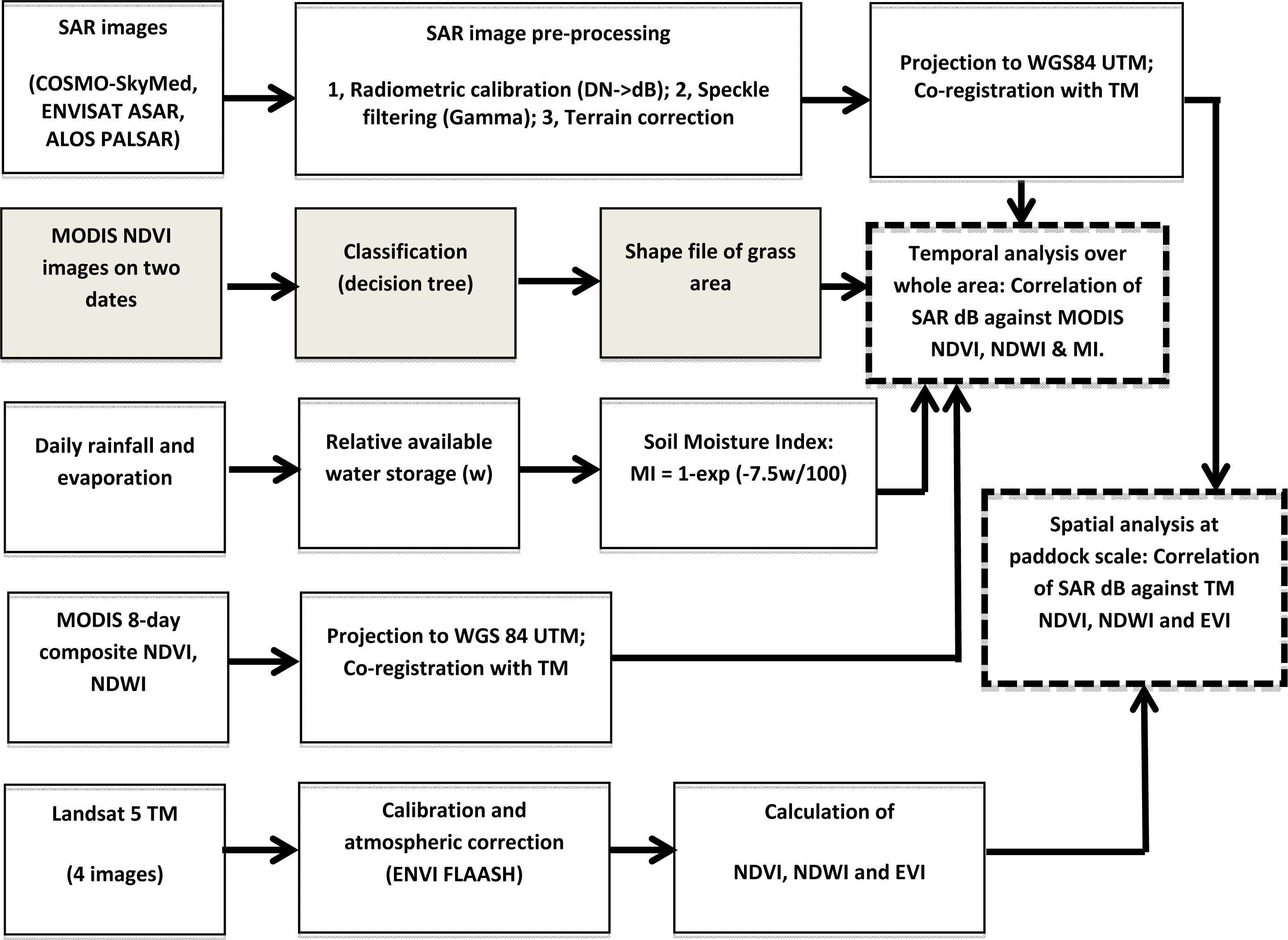
As presented in Figure 1, classification was first carried out using decision tree method over two MODIS NDVI images to extract the grass-only area from the study site. Then, over the grass area defined with the shapefile of the classification result, the time series of MODIS NDVI and NDWI, together with MI, were correlated with SAR HH backscattering coefficient (dB) to explore the potential of SAR in assessing temporal changes of grass biomass, water content, and soil moisture. Finally, Landsat TM NDVI, NDWI, and EVI of 29 paddocks were related to SAR HH backscatter to evaluate SAR’s potential for paddock-by-paddock variation of grass properties. This was conducted on two SAR imaging dates only, due to limited availability of corresponding Landsat TM images. Before the data analysis, pre-processing of optical and SAR data is necessary (see Figure 1).

2.1. Study Site and Data

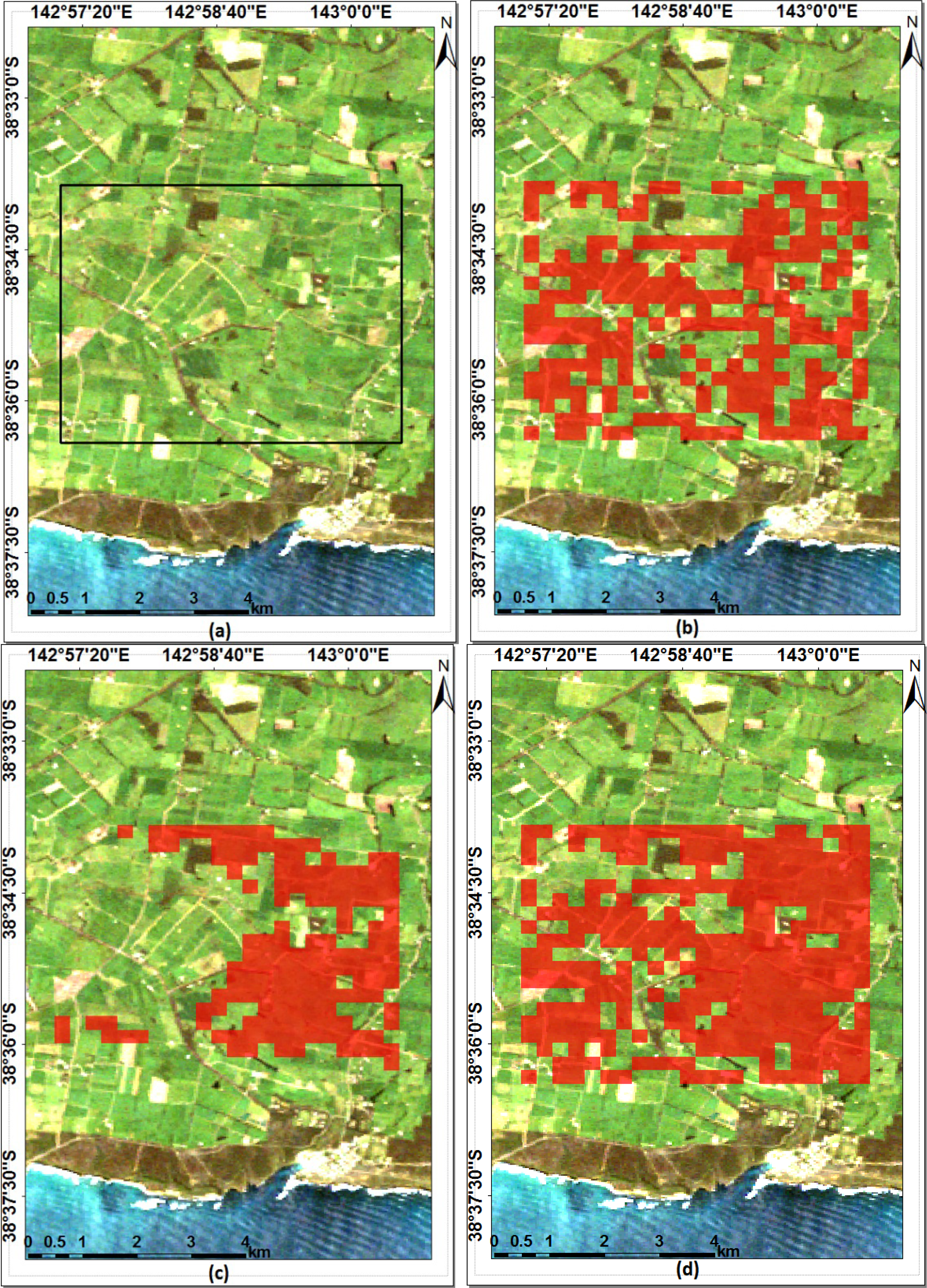
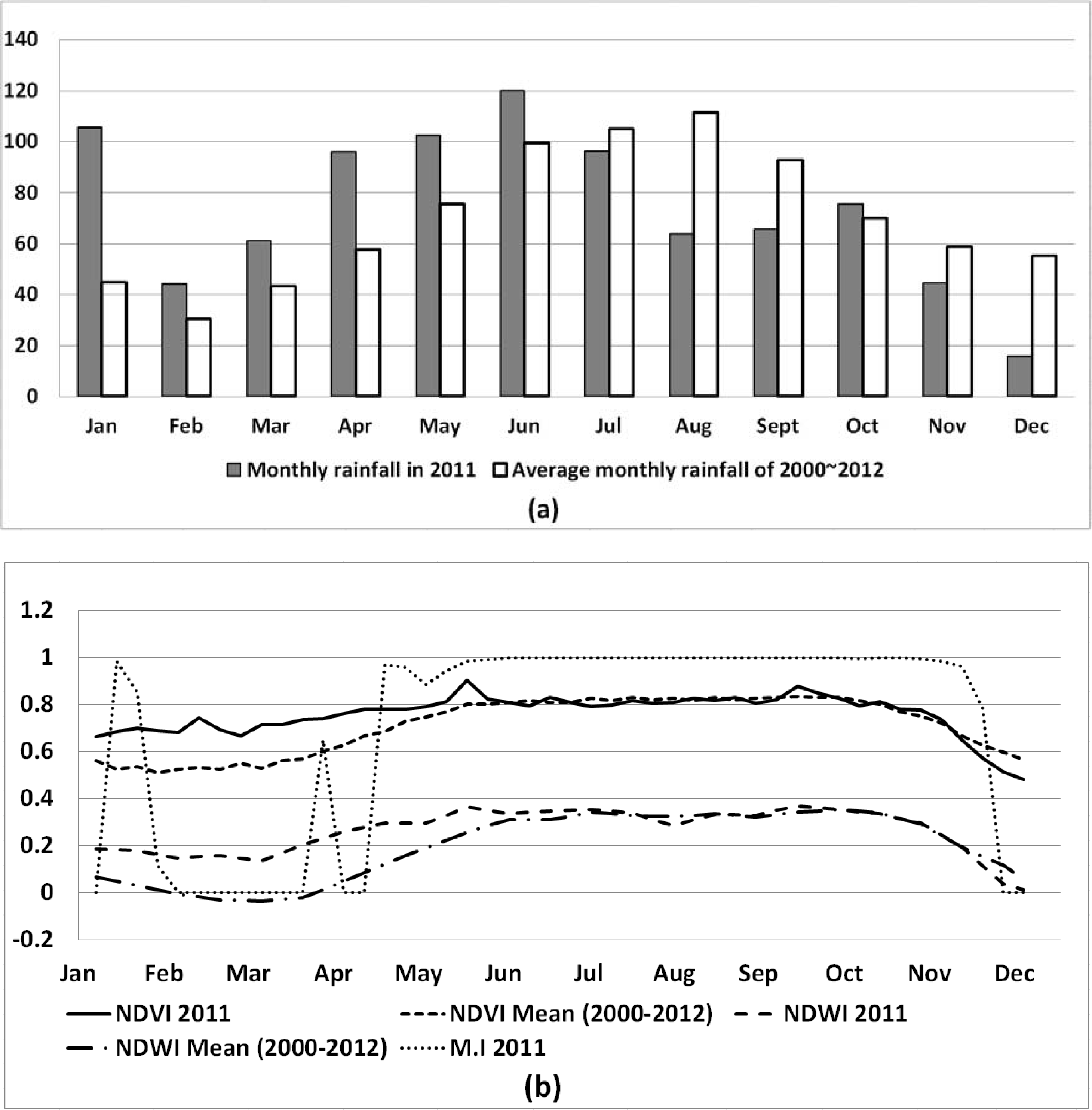
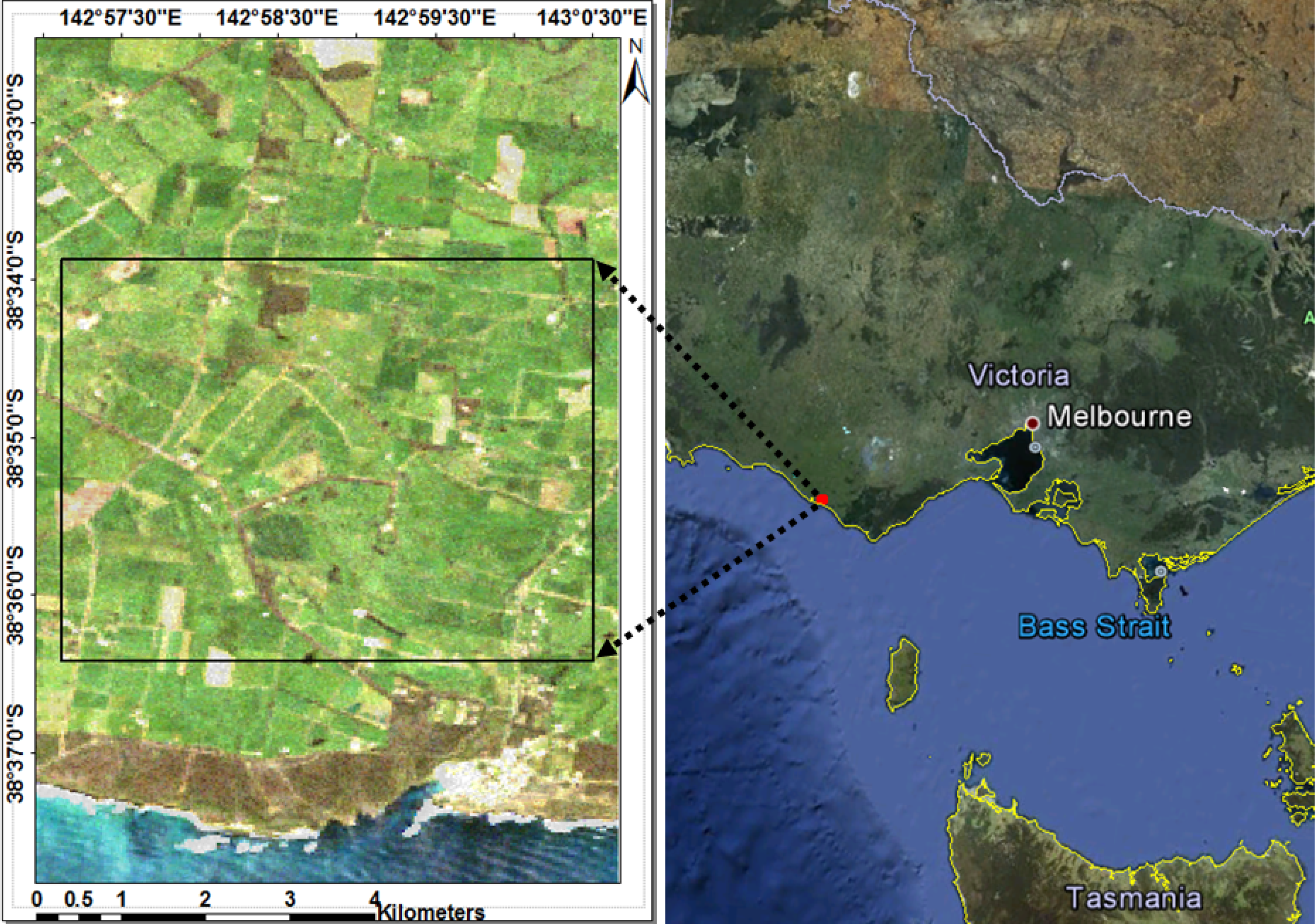
Figure 2 shows the study area (around 5 km × 5 km) in the Otway region, Southwest Victoria, Australia. Otway is one of the wettest parts in Victoria State. Grazing and dairy farming is an important signature of agriculture activity in this region. The annual dryland pasture zones in Otway are characterized by a distinct growing season, with a well-defined beginning and end. The season begins between April and June, depending upon the timing of the first significant rains, and ends in October or November. There was excessively plentiful rainfall in the dry season from the end of 2010 to the beginning of 2011, and consequently grass in the study area is presumed to stay green during that period.
MODIS eight-day composite NDVI images with 250 m resolution, during 13 years, from 2000 to 2012, were provided by the Department of United States Agriculture. These MODIS datasets are offering us the opportunity to derive the grass annual growth pattern. There are two Landsat images in the USGS archive that can be used to synchronize with SAR images to further analyze individual paddock’s biomass with a resolution of 30 m. The first Landsat 5 TM image was acquired on 19 October 2011, and matched up with ENVISAT ASAR image on 18 October 2011. The second Landsat 5 TM image was collected on 30 August 2007, corresponding to ALOS PALSAR image dated on 27 August 2007. Furthermore, the historical rainfall and evaporation data were obtained from the meteorological station Port Campbell Post Office (Station number: 90067, Lat: 38.62°S, Lon: 142.99°E).
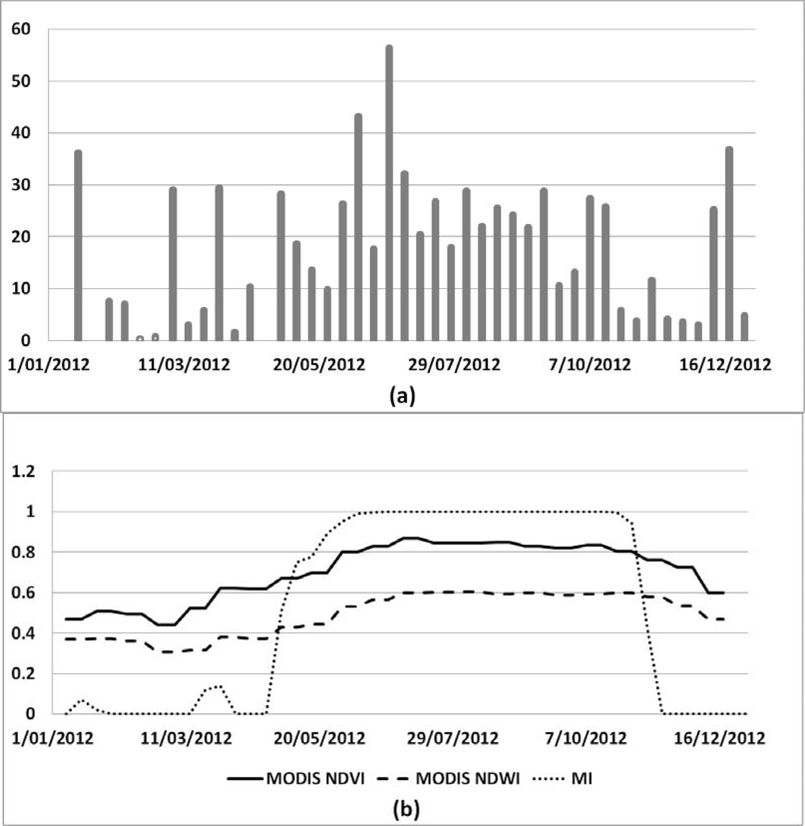
For SAR data, twenty-four X-band COSMO-SkyMed HH Stripmap images were acquired in 2012 with high temporal resolution (around eight days), and twenty-one of them were in growing season. The incidence angle was 30.5° on average in study area. The images were projected after pre-processing with pixel size of 15 m × 15 m. Following this, ten C-band ASAR Image Single Look Complex (IMS) HH images were obtained with incidence angle 33°, nine scenes with incidence angle 17°, ten scenes with incidence angle of 21°, and one image with an incidence angle of 24.5°. Finally, twenty-three scenes of L-band ALOS PALSAR Fine Mode Single Polarization (FBS) HH images, during 2007–2010, were acquired, and 10 of them were in growing season. The incidence angle was 34.3°. The pixel size of C- and L-band SAR images was 30 m × 30 m after image pre-processing. Table 1 is the list of all SAR images in details.

2.2. Synthetic Aperture Radar (SAR) Image Pre-Processing to Get Backscattering Coefficient (dB)

The SAR backscattering coefficient (sigma naught, dB) intensity image was obtained from single look complex (SLC) data through three steps of image processing, including radiometric calibration, spectral filtering and terrain correction. The NEST software, free software developed by the European Space Agency (ESA) for research, was used for this study. SAR data processing, which produces SLC images, does not include radiometric corrections and significant radiometric bias remains. It is therefore necessary to apply the radiometric correction to SAR SLC images so that the pixel values of the SAR intensity images truly represent the radar backscatter of the reflecting surface. Accurate calibration is also very important when multi-temporal data are used for applications. SAR intensity images have speckles that degrade the quality of the images and make interpretation of features more difficult. Speckle noise reduction can usually be addressed by adaptive filtering, and the Gamma Map filter is used here [31]. Due to topographical variations of a scene and the tilt of the satellite sensor, distances can be distorted in the SAR images because of the side-looking geometry of SAR images. Terrain corrections are intended to compensate for these distortions. Range Doppler ortho-rectification method [32] was used for geocoding SAR intensity images, and SRTM DEM with a three second resolution was used for terrain correction, and the ortho-rectified image was resampled with bilinear interpolation from the original to the final pixel size needed.

2.3. Calculation of Normalized Difference Vegetation Index (NDVI), Normalized Difference water index (NDWI) and Enhanced Vegetation Index (EVI)

It is necessary to remove atmosphere effect using the FLAASH tool in ENVI software after calibrating these Landsat TM images.
NDVI has been widely used for vegetation application, and the calculation of NDVI is as follows [33]:
NDVI = ( NIR Red ) / ( NIR + Red )
where Red and NIR stand for the spectral reflectance in the red and near infrared regions, respectively.
As for NDWI, the combination of the NIR with the Short Wave Infrared (SWIR) removes variations induced by leaf internal structure and leaf dry matter, and improves the accuracy in retrieving the vegetation water content [10,34]. The equation of NDWI is as follows:
NDWI = ( NIR SWIR ) / ( NIR + SWIR )
The computation of EVI is as follows [12]:
EVI = 2.5 × ( NIR Red ) / ( NIR + 6 × Red 7.5 × Blue + 1 )
where Blue stands for the spectral reflectance of blue regions.

2.4. Soil Moisture Index (MI) Estimated from Climate Data

Soil moisture index (MI) was computed based on water balance process (Equation (4)). MI scales the soil water availability between wilting point and field capacity to an index between 0 and 1.0 [35]. Different coefficients for sand, loam, and clay soil types are available for the equation to create the index. The dairy farmland in Otway is predominantly sandy loam and, therefore, defined which coefficient to use. The equation for moisture index is as follows:
MI = 1 e 7.5 × ( available water storage ) / 100
where available water storage was calculated based on daily rainfall and evaporation data which were collected from the meteorological station in Peterborough (The Lodge) (Number: 90191, Lat: 38.58°S, Lon: 142.87°E) close to the study area.

2.5. Classification of Study Area Using Decision Tree Method

Classification is essential to extract the grass zone since the study area is composed of multiple land use types: grass, houses, and batches of trees. MODIS NDVI data will be employed to describe the temporal changes of pasture biomass, hence classification was carried out using MODIS NDVI images. Nonetheless, there are mixed pixels on MODIS images since the coarser spatial resolution of 250 m makes it difficult to differentiate grass from the other land covers. On this basis, using one MODIS NDVI image for classification will easily lose some mixed pixels, which are dominantly covered by grass. In order to maximize the extraction of grass pixels, MODIS NDVI images on two dates (28 January and 19 October 2011) were used for classification, in dry and growing seasons accordingly, and then the two results were combined. The decision tree method was used for classification of each MODIS NDVI image, and the main feature for classification was NDVI mean value of each class. According to the combined classification results of two dates, a shapefile was extracted and used as area of interest for subsequent statistical analysis. A total of 29 paddocks were selected over the grass area for spatial analysis at the paddock scale.

2.6. Statistical Analysis

As mentioned in 
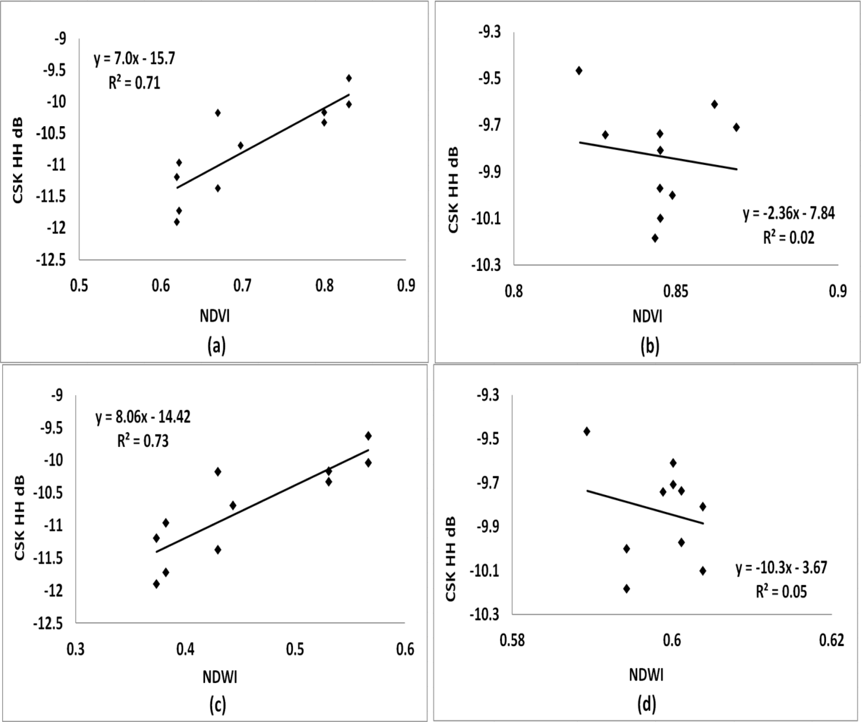
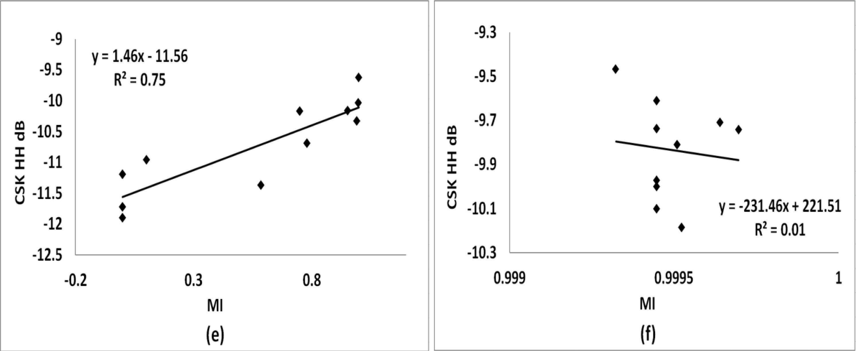
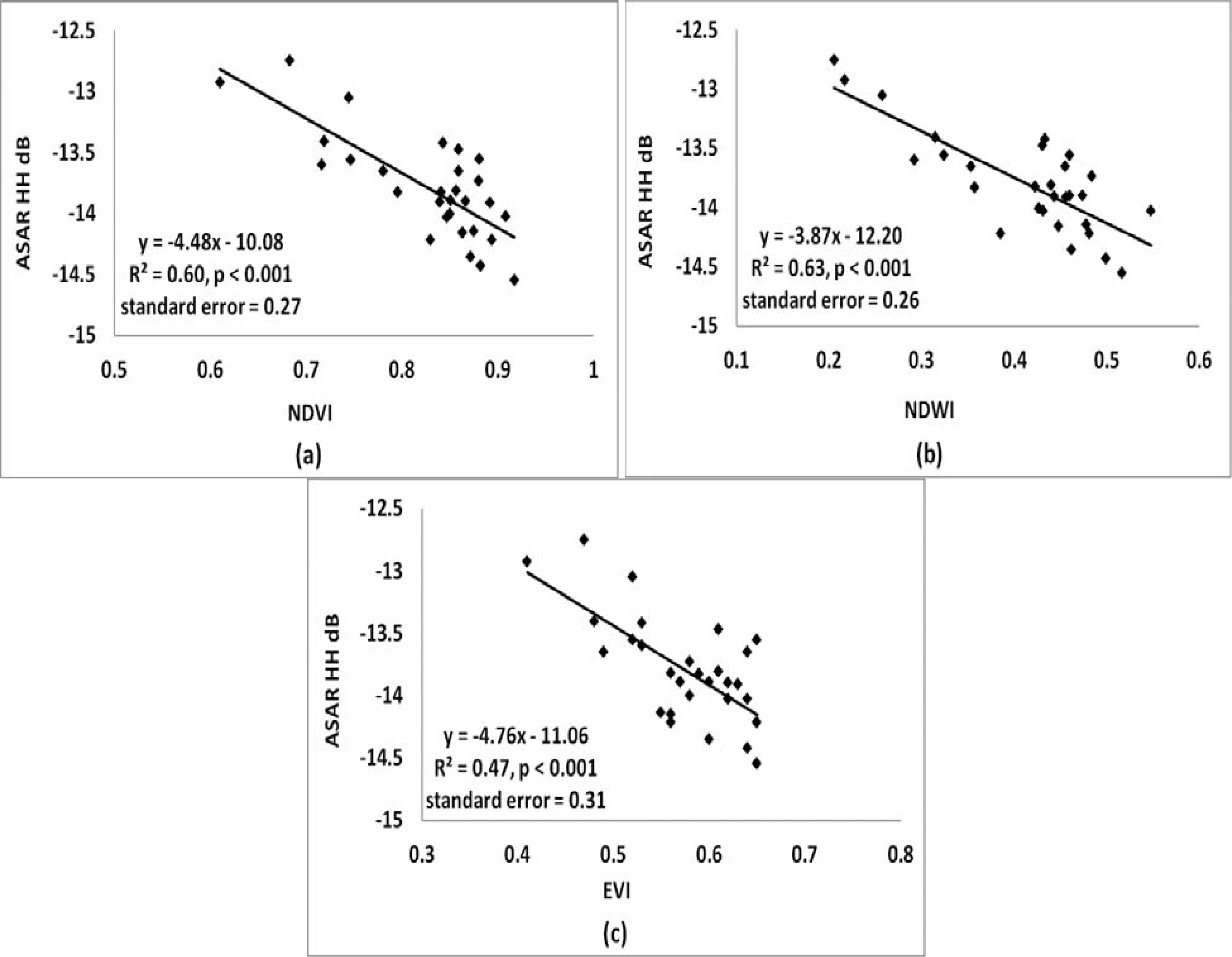
Figure 1, temporal analysis was conducted by correlating the mean value of SAR backscattering over the whole grass area with corresponding MI, MODIS NDVI, and NDWI. Paddock-by-paddock spatial correlation was based on the mean values of SAR backscattering of each paddock and TM vegetation indices (NDVI, NDWI, and EVI) accordingly. These relationships between SAR backscatter and optical vegetation index or soil moisture index are described by the following linear regression model:
dB = a 0 + a 1 D
where a0 and a1 are coefficients of the regression modeling. D is a vegetation index (NDVI, NDWI, EVI) or soil moisture index (MI). R-squared (R2) is the coefficient of determination in regression analysis, which describes how much of the backscatter variation was explained by the model in each case, and an R2 of 1 indicates that the regression line perfectly fits the data [36]. The p value describes the significance of the relationship [37], and a p value lower than 0.05 means a significant relationship at a 95% confidence interval. A lower p value means that the predictor in question has more impact on the model than the higher p values.

3. Results

3.1. Classification

In the study area, there are totally 19 × 20 pixels on MODIS NDVI image (pixel size: 250 m). After classification using decision tree, 227 grass pixels were obtained on 28 January and 150 grass pixels on 19 October 2011 (Figure 3b,c). From the result figures we can see, trees, and houses were removed, but some grass dominated pixels were also removed by mistake. This problem was even worse on 19 October 2011, since in the peak season, grass was not easily differentiated from trees and houses with greening. Therefore, the results of two dates were combined and a total of 257 grass pixels were obtained. A shapefile was generated from the results and all subsequent correlation analysis was based on the grass area represented by the shapefile (Figure 3).

3.2. Constellation of small Satellites for the Mediterranean Basin Observations (COSMO-SkyMed) Results

In 2012, grass started growing at the end of March and biomass reached peak level at the beginning of July. Peak season sustained until the end of October when soil and grass began drying up. This growth trend of grassland was largely related to the amount of rainfall and the subsequent soil moisture (Figure 4). A total of 24 CSK images were acquired in 2012 and as many as 21 of them were in growing season, which made it possible to conduct a detailed study of temporal changes of pasture in growing season.
The time series of CSK HH backscattering coefficient on 24 dates over grass area, together with MODIS NDVI, NDWI, and soil moisture index, were presented in Figure 5. These CSK images were divided into three groups: dry season (three dates in total, from 25 February to 20 March 2012), early growing season (10 dates total, from 28 March to 24 June 2012) and peak season (11 dates altogether, from 2 July to 20 September 2012) (see Figure 5). It was observed that the variation of CSK HH dB was great, especially in dry season and early growing season. For the three dates in dry season, CSK HH backscattering coefficient changed positively with rainfall and soil moisture. The backscattering coefficient increased dramatically from −11.40 dB on 25 February to the peak value of −8.54 dB on 20 March. Meanwhile, the soil moisture index increased from 0 to 0.12 accordingly, and there was rainfall on 20 March when the peak SAR value was observed. In the subsequent three dates in early growing season, CSK backscatter kept decreasing with soil moisture. Based on these observations, it was clear that the change of soil moisture in dry season and at the beginning of growing season is detectable by using CSK backscatter at HH polarization. This indicates that dry grass and newly grown young grass had limited effects upon SAR scattering, whereas soil moisture imposed substantial influence. When it comes to the whole period of early growing season, CSK HH backscattering appeared to rise with grass growth until before peak season. This trend in early growing season can be further explored by means of linear regression, together with peak season. For peak season with saturated soil moisture, NDVI, and NDWI stood at a high level without obvious changes, but CSK backscattering coefficient fluctuated dramatically (Figure 5). This clearly demonstrates that CSK signal has potential to detect grass of high biomass while NDVI and NDWI cannot work well due to saturation problems.
Linear regression was conducted between time series of CSK HH backscattering and MODIS NDVI, NDWI, as well as MI, for both early growing season and peak season. The coefficient of determination (R2) and p value of linear regression were given in Table 2 and Figure 6. It was found that, in early growing season, CSK HH dB was positively related to NDVI (R2 = 0.71), NDWI (R2 = 0.73), and soil moisture index (MI) (R2 = 0.75). In contrast, in peak season when biomass reached a high level, CSK backscattering changed intensively, and the correlation of CSK backscatter against NDVI, NDWI, or MI was very weak (R2 = 0.01–0.05). This is probably related to the fact that CSK signal has more capability than optical indices to estimate properties of grass of high biomass. Meanwhile, fluctuation of CSK signal was also largely attributed to rainfall, which actually happened in six out of the 10 dates of peak season. Water on leaves after rainfall can cause substantial change of CSK backscattering coefficient [30]. For the other four dates, without rainfall, in peak season (see blue colored points in Figure 5), the CSK backscatter increased while NDVI decreased due to grazing or cutting activities. To sum up, CSK HH backscattering coefficient can be used to estimate the temporal changes (e.g., biomass, plant water content) from the beginning of growing season until before peak season, despite its concurrent sensitivity to soil moisture. During peak season, CSK backscattering is able to detect grazing or mowing activities on non-rainy dates, but this ability weakens when rainfall happens. Positive relationship between SAR signal and biomass in early stage of growing season is due to the lower biomass of sparse grass, which made surface scattering dominant in scattering mechanism. In comparison, in peak season, SAR backscattering changes negatively with biomass because volume scattering dominates when biomass becomes higher.

3.4. Environmental Satellite Advanced Synthetic Aperture Radar (ENVISAT ASAR) Results

3.4.1. Temporal Analysis of Environmental Satellite Advanced Synthetic Aperture Radar (ENVISAT ASAR) HH Polarization Backscattering Coefficient against Moderate Resolution Imaging Spectroradiometer (MODIS) Normalized Difference Vegetation Index (NDVI), Normalized Difference Water Index (NDWI) and Soil Moisture Index (MI)

The study area of grassland in Otway was influenced by the particularly abundant rainfall in 2011. The monthly rainfall from January to June, in 2011, was much higher than the average of years 2000–2012, thus the NDWI (plant water content) in the corresponding period of 2011 was much higher than the average of years 2000–2012, so was the NDVI (2011: 0.68–0.81; 2000–2012: 0.11–0.77) (Figure 7). In 2011, grass started growing (NDVI = 0.685) as early as in March due to extraordinarily plenty rainfall, and then reached peak biomass level (NDVI = 0.8–0.9) at the beginning of June. Peak season sustained until the end of October when soil and grass began drying up. The time series of ENVISAT ASAR HH backscattering coefficient (dB) of 29 dates for the study area, are presented in Figure 8, together with MODIS NDVI, NDWI, and MI.
The time series of ASAR backscattering coefficient with incidence angle of 33° is presented in Figure 8a, and ASAR backscattering with incidence angle of 17° and 21° is shown in Figure 8b. For the incidence angle of 33°, it was observed that from dry season to early growing season, ASAR HH backscattering coefficient changes positively with soil moisture. For example, the peak value (−12.78 dB) on 13 January, 2011 (the first point in Figure 8a), was related to the high soil moisture (MI = 0.98) on that date. When soil moisture index (MI) dropped to 0.58 on 24 January, 2011, ASAR backscatter decreased sharply to −15.07 dB. For the whole growing season, soil moisture maintained nearly saturated, whereas ASAR HH backscatter fluctuated significantly. Biomass and water content, represented by NDVI and NDWI, might be the factors causing the fluctuation and should be given some attention in subsequent linear regression. For incidence angles of 17° and 21°, the backscattering coefficient in growing season (−12.91–−10.18 dB) is bigger overall than in drying season (−14.97–−12.35 dB). Aside from seasonal trends, fluctuations were also observed both in growing and dry season. For example, the bigger backscattering (−12.35 dB) on 15 March, 2012, in drying season (the last point in Figure 8a) is possibly attributed to the rainfall (2.6 mm) on that day. Grazing and regrowth events also play an important role in these fluctuations. Further investigation of these correlations can be performed by means of a linear regression model. In addition, from Figure 8a,b we can see that, in peak season, ASAR signal exhibited a change curve with a well-defined peak, while NDVI and NDWI maintained at a high level due to saturation. This may prove that ASAR HH backscattering coefficient has an advantage over optical in detecting high biomass of grass.
All ASAR images were divided into four groups based on different incidence angles: 33°, 17°, 21°, and 24.5°. The four groups had 10, 9, 10, and 1 scene of images, respectively. For the first three groups, linear regression model was carried out between time series of ASAR HH dB and MODIS NDVI, NDWI, together with MI, for the whole study area. Additionally, for the incidence angle of 33°, eight out of 10 images were in growing season, and for incidence angles of 17° and 21°, a total of seven images were in growing season. Then, for these two growing season groups, a linear regression model was also conducted. The modeling results for the whole year and growing season were presented in Table 3.
The whole time series of ASAR HH backscatter with incidence angle of 33° was moderately correlated with NDVI (R2 = 0.56, p < 0.01), but not with NDWI and MI. On the other hand, with smaller incidence angle of 17° and 21°, the relationship between ASAR signal and NDVI (biomass) became weaker while it was the opposite for soil moisture. When we focused on growing season, ASAR HH backscattering with an incidence angle of 33° maintained the moderate sensitivity for temporal variation of biomass (R2 = 0.48, p = 0.05), while with incidence angles of 17° and 21° it did not show any capability for biomass or soil moisture. In growing season, with small incidence angles of 17° and 21°, the scattering process becomes quasi-specular, where small facets of grass leaves align normally to the incidence waves. This helps explain why the sensitivity of data to the scene is very low. To conclude, ASAR HH backscattering coefficient with an incidence angle of 33° was able to detect temporal variation of grass biomass. ASAR HH dB with incidence angles 17° and 21°, however, were able to detect big seasonal changes of soil moisture only. Results from earlier studies [38] largely support these observations.

3.4.2. Spatial Analysis of Environmental Satellite Advanced Synthetic Aperture Radar (ENVISAT ASAR) HH dB against Landsat 5 Thematic Mapper (TM) Normalized Difference Vegetation Index (NDVI), Normalized Difference Water Index (NDWI) and Enhanced Vegetation Index (EVI)

For spatial analysis over 29 paddocks, the ASAR HH image with incidence angle of 24.5° was acquired on 18 October 2011, and one Landsat 5 TM image was collected on 19 October, 2011. The linear regression models between ASAR HH dB and TM NDVI, NDWI and EVI are presented in Figure 9a–c, respectively. This was the end of peak season, with nearly saturated soil (MI = 0.997) and high biomass (NDVI mean = 0.79). The dynamic range in the ASAR backscatter is quite small (less than 2 dB, from −14.6–−12.7 dB), thus the accuracy of the backscattering coefficient should be guaranteed by accurate calibration, which was already addressed in image preprocessing. The large range of NDVI (0.61–0.92) indicates significant variation of biomass at the paddock scale and the lower NDVI values such as 0.61 are probably related to grazing or mowing events. It is noticed that the paddocks with lower NDVI values tend to have higher SAR dB values (Figure 9a), and this is probably due to grazing activities, which weakened volume scattering and strengthened the soil-grass interaction by reducing leaves. The linear relationship gave moderate R2 value of 0.63 between ASAR dB and NDWI, followed by NDVI (R2 = 0.60) and EVI (R2 = 0.47). To sum up, at the end of peak season, paddock scale variation of water content and biomass, caused by growth condition or grazing events, can be detected by ASAR HH backscatter. The backscatter changes negatively with biomass and water content. All the results were based on incidence angle of 24.5° and saturated soil moisture.

3.5. Advanced Land Observation Satellite Phased Array Type L-band Synthetic Aperture Radar (ALOS PALSAR) Results

3.5.1. Temporal Analysis of Environmental Satellite Advanced Synthetic Aperture Radar (ALOS PALSAR) HH dB against Moderate Resolution Imaging Spectroradiometer (MODIS) Normalized Difference Vegetation Index (NDVI), Normalized Difference Water Index (NDWI), and Soil Moisture Index (MI)

The time series of ALOS PALSAR HH backscattering coefficient (dB) on 23 dates over the whole study area of grass, together with corresponding MODIS NDVI, NDWI, and soil moisture index, are presented in Figure 10. PALSAR HH backscattering appeared higher in growing season, and lower in dry season. Linear relationship was investigated between SAR signal and multiple indices (MI, MODIS NDVI, and NDWI), and the coefficient of determination (R2) and p value were given in Table 4. The whole time series of PALSAR HH dB was strongly related to NDVI (R2 = 0.79), and weakly correlated to NDWI (R2 = 0.46) and MI (R2 = 0.38). For time series in the growing season, weaker relationships were achieved between PALSAR HH dB and NDVI (R2 = 0.49) and MI (R2 = 0.45), followed by NDWI (R2 = 0.38). Biomass and soil moisture are therefore two important factors involving in SAR scattering, and they should be considered when using PALSAR at HH polarization for grassland seasonal changes.

3.5.2. Spatial Analysis of Advanced Land Observing Satellite Phased Array Type L-band Synthetic Aperture Radar (ALOS PALSAR) HH dB against Landsat 5 Thematic Mapper (TM) Normalized Difference Vegetation Index (NDVI), Normalized Difference Water Index (NDWI), and Enhanced Vegetation Index (EVI)

Spatial analysis over 29 paddocks was carried out based on ALOS PALSAR HH image on 27 August 2007 and Landsat 5 TM image on 30 August 2007. SAR backscattering was related to TM NDVI, NDWI and EVI by means of linear regression analysis (Figure 11a–c). NDVI ranges from 0.64 to 0.92 and PALSAR HH dB is from −11.98 to −7.59 dB, which indicates a large range of paddock-by-paddock variation of biomass and SAR backscattering coefficient (Figure 11a). Lower NDVI value, which illustrates worse growth conditions or grazing activities, corresponds to higher PALSAR HH dB value. Therefore, paddocks with poor grass growth and paddocks after grazing can be located by bigger PALSAR backscatter. This pair of dates was in peak growing season with saturated soil moisture (MI = 0.99) and high biomass, and the relationships were significant (p < 0.05) but very weak (R2 = 0.15–0.19). This further proved that PALSAR HH backscattering has limited potential for grass biomass since soil moisture is important in scattering of PALSAR HH.

4. Discussions

The statistical results over grass area have shown that HH polarization of COSMO-SkyMed (X-band), ENVISAT ASAR (C-band) and ALOS PALSAR (L-band) is able to measure temporal and spatial variation of pasture biomass, plant water content, and soil moisture at the paddock and large scale. This capability of SAR depends on several factors including growth stage, soil moisture, incidence angle, and wavelength.
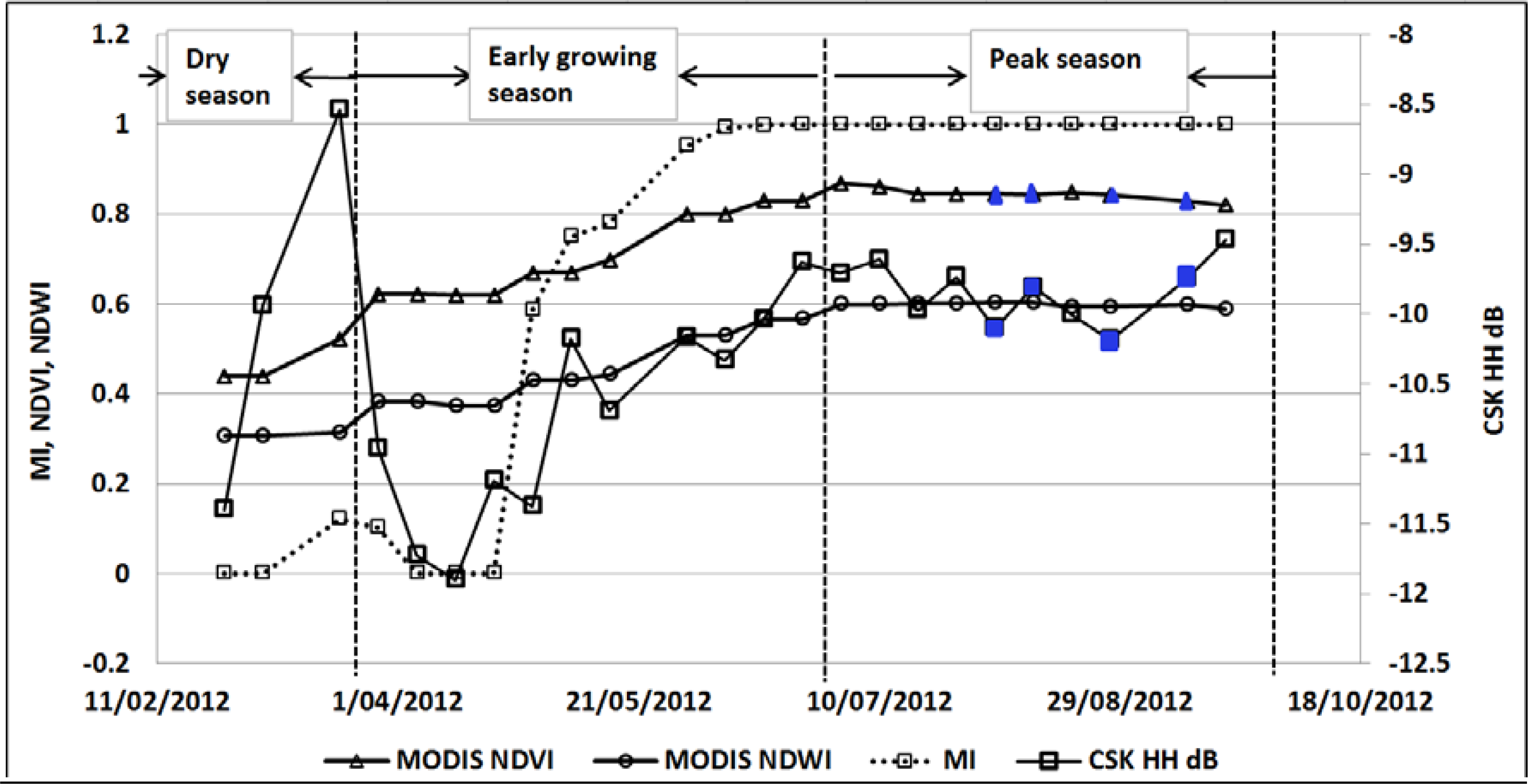
High revisit frequency of remote sensing images is very important for pasture monitoring. A total of 24 CSK, 30 ENVISAT ASAR, and 23 ALOS PALSAR images were collected in this study. It needs to be pointed out that, among 24 scenes of CSK images, as many as 21 of them were in growing season for the year of 2012. In contrast, only eight (or seven) scenes of ENVISAT ASAR and 10 scenes of ALOS PALSAR images were in growing season, and scattered in two and five years respectively. In a word, the large number and high temporal resolution (eight days) of CSK HH images made it possible to study its temporal variation in two different growth stages: early growing season and peak growing season. CSK HH backscatter with an incidence angle of 30.5° has shown strong reliability to detect temporal changes of pasture biomass in early growing season. However, in peak season, the accuracy of CSK HH on detecting biomass variation or grazing was undermined by rainfall events. The effect of rainfall on CSK HH signal can also be observed in the dry season. Supporting this, a previous study over shrub and grassland areas found that VV polarization of CSK increased significantly due to rainfall [
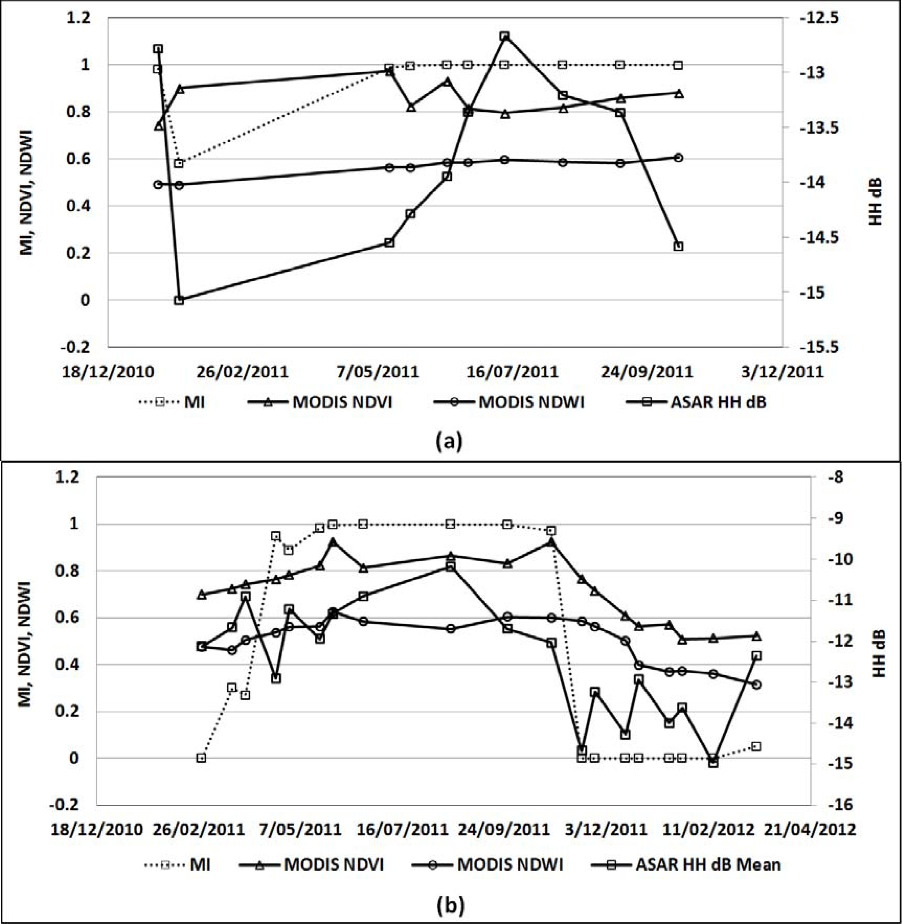
30]. Therefore, non-rainfall dates are preferred when using CSK backscattering for pasture monitoring. When it comes to ENVISAT ASAR, HH backscatter with an incidence angle 33° has moderate reliability for pasture biomass in growing season, while ASAR with incidence angles of 17° and 21° are not suitable for this purpose. This is in line with the result of a study that, when steeper incidence angles such as 23° are used in ERS and ENVISAT, the direct returning signal from the ground is strong and shows a clear dependence on soil moisture [38]. Therefore, larger incidence angle should be selected when using ASAR HH for measuring pasture biomass. As far as L-band is concerned, ALOS PALSAR data at HH polarization appears to be weak for sensing both temporal and spatial changes of biomass. This can be related to the fact that L-band radar has strongest penetration ability, thus the soil condition involves in scattering signal strongly.
SAR backscattering signal differs at various bands. The longest wavelength SAR has the strongest penetration ability, while the short one is reversed. For soil covered with grass in case of low frequency (C and L-band), the total backscattering is a combination of contributions from soil and vegetation layer, while in case of high frequency (X-band), the total backscattering is the contribution of vegetation layer only. This helps explain why CSK (X-band) backscattering in this study was largely affected by rainfall and consequently the water standing on the leaves, both in dry season and peak growing season. Therefore, we could interpret that, for temporal changes of plant water content, X-band shows its strong sensitivity to plant water content while C- and L-band cannot. The influence of rainfall upon X-band was observed for both dry and growing season, while the impact on C-band was for dry season only. It seems that the shorter the wavelength is, the more the water after rainfall will bring to SAR signal. A reasonable explanation is that SAR backscatter with shorter wavelength reflects more information about grass canopy, moreover, in dry season, it will focus on water existing on leaves rather than plant water content which is low in dry season. Therefore, when X- and C-band are used for dry grass monitoring in dry season, the dates without rainfall should be selected for experiment. In addition, in peak growing season, non-rainfall days should be selected if X-band data is used for grass biomass monitoring. Furthermore, the interaction of SAR with vegetation strongly depends on the kind of vegetation. The interaction of radar signal with short vegetation (such as grass) mainly results in diffuse scattering [30]. This helps explain the phenomenon that, in peak season when biomass is high, HH backscattering coefficient at X-, C-, and L-band decreased with biomass and plant water content. It needs to be pointed out that, both X- and C-band backscattering coefficient showed strength in measuring high biomass of grass in peak season when optical indices saturate. We did not see similar phenomenon from L-band data because of temporally sparse images, but we may get observations when dense images are available in future.
Apart from the potential of SAR for pasture biomass and plant water content, its capability to detect soil moisture is also of practical importance for pasture management. Incidence angle and wavelength are important factors affecting this ability. With an incidence angle of 30.5°, CSK (X-band) was able to detect soil moisture in dry season and early growing season, due to the limited influence of dry or sparsely short green grass upon CSK signal. However, in peak growing season, green grass became dense and high and then CSK signal focused upon grass properties rather than soil moisture due to its weak penetration ability. ENVISAT ASAR (C-band) appeared to be moderately sensitive to seasonal changes of soil moisture when the incidence angle was small (e.g., 17°–21°), and the sensitivity became very weak when the incidence angle was bigger (e.g., 33°). ALOS PALSAR (L-band) maintained moderate ability to temporal variation of soil moisture even if the incidence angle was bigger (34.3°), which indicated that L-band has advantage in detection of soil moisture. These are comparable to the results of a previous study using radar scatterometer that, for HH polarization at the L-band and C-band over grass-covered fields in Oklahoma in the US, the coherent scattering from soil surface is very important at angles near nadir, while the vegetation volume scattering is dominant at larger incidence angles (>30°) [39].

5. Conclusions

As pasture is one dominant land type used in Australia, how to better manage it is of great importance for profitability and sustainability. Optical remote sensing shows promise in providing information for pasture management, but its ability is hampered by clouds and low resolution. Due to the inference to clouds, higher spatial resolution, and the ability to detect moisture content of pasture, SAR is considered a perfect complement to optical for efficient pasture monitoring at the paddock scale. This study aims to investigate the feasibility of using multi-temporal COSMO-SkyMed (X-band), ENVISAT ASAR (C-band), and ALOS PALSAR (L-band) images at HH polarization for monitoring pasture in Otway, Australia. To achieve this, SAR backscatter coefficients were correlated to spectral vegetation indices (NDVI, NDWI, and EVI) as well as soil moisture index (MI). Spectral vegetation indices and MI were used to assist our understanding of the ability of SAR data at X-, C-, and L-band to measure pasture biomass, plant water content and soil moisture. This method is an efficient and cost-effective way to study the potential of SAR for pasture monitoring.
This study was the first attempt to analyze, at both the temporal and spatial domains, the pasture properties in Otway, Australia, using SAR data acquired with three different bands. Although spatial analysis need to be further investigated with ground supporting data, our results clearly demonstrated the feasibility of using multiple SAR data for pasture monitoring. For all three bands, dramatically higher SAR backscatter on one specific paddock illustrates grazing or mowing activities, and lower backscatter implies higher biomass of grass. X-band is supposed to have the advantage in terms of short wavelength suitable for grass detection, but X-band signal fluctuates dramatically with water on leaves after rainfall, while C- and L-band appeared more stable. SAR, particularly at X- and C-band, showed advantage over NDVI in detecting high biomass in peak season, which provides a solution to the problem of saturation of optical index. The quantitative relationship between SAR signal and high biomass can be investigated in further studies if ground data are acquired. The medium penetration ability of C-band can be used to compensate X-band for estimating biomass on rainy dates while high penetration L-band can focus on soil moisture. All the results are of practical significance for local pasture management and also provide useful information for similar ecosystems in other places.
In future study, high resolution optical images SPOT 5 or ground data can be acquired on or close to SAR imaging dates, in order to achieve more comprehensive results. Apart from HH polarization investigated in this study, other polarizations can be used and compared in further research. It is well known that frequent observations are important for pasture monitoring, and SAR images at various bands can be combined with optical images to achieve near real-time observation eventually. When it comes to pasture properties over large area, it is worthwhile trying to evaluate the results with E.M. models and use inversion algorithms for estimating the vegetation and soil parameters. Additionally, ground measurements of dry biomass are essential for investigation of the potential of X- and C-band to measure dry grass.

Acknowledgments

This research was supported under Australian Research Council's Linkage funding scheme (project number LP0882595) and Discovery funding scheme (project number DP130101694). The Department of Agriculture and Food Western Australia (DAFWA) and the Commonwealth Scientific and Industrial Research Organization (CSIRO) are gratefully acknowledged as project partners.
The authors wish to thank the Earth Remote Sensing Data Analysis Center (ERSDAC) and the European Space Agency (ESA) for providing the ALOS PALSAR and ENVISAT ASAR data, respectively. METI and JAXA retain ownership of the ALOS PALSAR original data. The authors would also like to thank e-GEOS group, Italy for providing imagery of COSMO-SkyMed for this study. The authors acknowledge the U.S. Geological Survey for providing Landsat and MODIS data used in this study.

Conflict of Interest

The authors declare no conflict of interest.

References

  1. McNeill, S.; Pairman, D.; Belliss, S.; Dalley, D.; Dynes, R. Estimation of Pasture Biomass Using Dual-Polarisation Radar Imagery—A Preliminary Study. Proceedings of 23rd International Conference on Image and Vision Computing, Christchurch, New Zealand, 26–28 November 2008; pp. 1–6.
  2. Tieszen, L.L.; Reed, B.C.; Bliss, N.B.; Wylie, B.K.; De Jong, D.D. NDVI, C3 and C4 production, and distributions in Great Plains grassland land cover classes. Ecol. Appl 1997, 7, 59–78. [Google Scholar]
  3. Hill, M.; Donald, G.; Vickery, P. Relating radar backscatter to biophysical properties of temperate perennial grassland. Remote Sens.. Environ 1999, 67, 15–31. [Google Scholar]
  4. Ferreira, L.G.; Fernandez, L.E.; Sano, E.E.; Field, C.; Sousa, S.B.; Arantes, A.E.; Araújo, F.M. Biophysical properties of cultivated pastures in the Brazilian savanna biome: An analysis in the spatial-temporal domains based on ground and satellite data. Remote Sens 2013, 5, 307–326. [Google Scholar]
  5. Schino, G.; Borfecchia, F.; De Cecco, L.; Dibari, C.; Iannetta, M.; Martini, S.; Pedrotti, F. Satellite estimate of grass biomass in a mountainous range in central Italy. Agroforest. Syst 2003, 59, 157–162. [Google Scholar]
  6. Hill, M.J.; Donald, G.E.; Hyder, M.W.; Smith, R.C.G. Estimation of pasture growth rate in the south west of Western Australia from AVHRR NDVI and climate data. Remote Sens. Environ 2004, 93, 528–545. [Google Scholar]
  7. Donald, G.; Gherardi, S.; Edirisinghe, A.; Gittins, S.; Henry, D.; Mata, G. Using MODIS imagery, climate and soil data to estimate pasture growth rates on farms in the south-west of Western Australia. Anim. Prod. Sci 2010, 50, 611–615. [Google Scholar]
  8. Edirisinghe, A.; Hill, M.; Donald, G.; Hyder, M. Quantitative mapping of pasture biomass using satellite imagery. Int. J. Remote Sens 2011, 32, 2699–2724. [Google Scholar]
  9. Laurila, H.; Karjalainen, M.; Kleemola, J.; Hyyppä, J. Cereal yield modeling in finland using optical and radar remote sensing. Remote Sens 2010, 2, 2185–2239. [Google Scholar]
  10. Gao, B.C. NDWI—A normalized difference water index for remote sensing of vegetation liquid water from space. Remote Sens. Environ 1996, 58, 257–266. [Google Scholar]
  11. Gu, Y.; Brown, J.; Verdin, J.; Wardlow, B. A five-year analysis of MODIS NDVI and NDWI for grassland drought assessment over the Central Great Plains of the United States. Geophys. Res. Lett 2007, 34, L06407. [Google Scholar]
  12. Huete, A.; Didan, K.; Miura, T.; Rodriguez, E.P.; Gao, X.; Ferreira, L.G. Overview of the radiometric and biophysical performance of the MODIS vegetation indices. Remote Sens. Environ 2002, 83, 195–213. [Google Scholar]
  13. Matsushita, B.; Yang, W.; Chen, J.; Onda, Y.; Qiu, G. Sensitivity of the Enhanced Vegetation Index (EVI) and Normalized Difference Vegetation Index (NDVI) to topographic effects: A case study in high-density cypress forest. Sensors 2007, 7, 2636–2651. [Google Scholar]
  14. Dusseux, P.; Gong, X.; Corpetti, T.; Hubert-Moy, L.; Corgne, S. Contribution of Radar Images for Grassland Management Identification. Proceedings of SPIE (International Society for optics and photonics) on Remote Sensing, Edinburgh, UK, 24–27 September 2012; pp. 1–7.
  15. Schmullius, C.; Furrer, R. Frequency dependence of radar backscattering under different moisture conditions of vegetation-covered soil. Int. J. Remote Sens 1992, 13, 2233–2245. [Google Scholar]
  16. Moreau, S.; Le Toan, T. Biomass quantification of Andean wetland forages using ERS satellite SAR data for optimizing livestock management. Remote Sens. Environ 2003, 84, 477–492. [Google Scholar]
  17. Attema, E.; Ulaby, F.T. Vegetation modeled as a water cloud. Radio Sci 1978, 13, 357–364. [Google Scholar]
  18. Oh, Y.; Sarabandi, K.; Ulaby, F.T. An empirical model and an inversion technique for radar scattering from bare soil surfaces. IEEE Trans. Geosci. Remote Sens 1992, 30, 370–381. [Google Scholar]
  19. Ulaby, F.T.; Bradley, G.A.; Dobson, M.C. Microwave backscatter dependence on surface roughness, soil moisture, and soil texture: Part II-vegetation-covered soil. IEEE Trans. Geosci. Electro 1979, 17, 33–40. [Google Scholar]
  20. Ferrazzoli, P.; Paloscia, S.; Pampaloni, P.; Schiavon, G.; Sigismondi, S.; Solimini, D. The potential of multifrequency polarimetric SAR in assessing agricultural and arboreous biomass. IEEE Trans. Geosci. Remote Sens 1997, 35, 5–17. [Google Scholar]
  21. Fung, A.K.; Chen, K.-S. Microwave Scattering and Emission Models and Their Applications; Artech House Publishers: Boston, MA, USA, 1994. [Google Scholar]
  22. Wu, T.-D.; Chen, K.-S. A reappraisal of the validity of the IEM model for backscattering from rough surfaces. IEEE Trans. Geosci. Remote Sens 2004, 42, 743–753. [Google Scholar]
  23. Paloscia, S.; Pettinato, S.; Santi, E.; Notarnicola, C.; Pasolli, L.; Reppucci, A. Soil moisture mapping using Sentinel-1 images: Algorithm and preliminary validation. Remote Sens. Environ 2013, 134, 234–248. [Google Scholar]
  24. Santi, E.; Fontanelli, G.; Montomoli, F.; Brogioni, M.; Macelloni, G.; Paloscia, S.; Pettinato, S.; Pampaloni, P. The Retrieval and Monitoring of Vegetation Parameters from COSMO-SkyMed Images. Proceedings of IEEE International Geoscience and Remote Sensing Symposium (IGARSS), Munich, Germany, 22–27 July 2012; pp. 7031–7034.
  25. Stolz, R.; Mauser, W. Evaluation of ERS Data for Biomass Estimation of Meadows. Proceedings of the Third ERS Symposium on Space at the Service of Our Environment, Florence, Italy, 14–21 March 1997; pp. 203–207.
  26. McNairn, H.; Champagne, C.; Shang, J.; Holmstrom, D.; Reichert, G. Integration of optical and Synthetic Aperture Radar (SAR) imagery for delivering operational annual crop inventories. ISPRS J. Photogramm 2009, 64, 434–449. [Google Scholar]
  27. McNairn, H.; Shang, J.; Champagne, C.; Jiao, X. TerraSAR-X and RADARSAT-2 for Crop Classification and Acreage Estimation. Proceedings of IEEE International Geoscience and Remote Sensing Symposium (IGARSS), Cape Town, South Africa, 12–17 July 2009; Volume II. pp. 898–901.
  28. McNeill, S.; Pairman, D.; Belliss, S.; Dalley, D.; Dynes, R. Robust Estimation of Pasture Biomass Using Dual-Polarisation TerrASAR-X Imagery. Proceedings of IEEE International Geoscience and Remote Sensing Symposium (IGARSS), Honolulu, HI, USA, 25–30 July 2010; pp. 3094–3097.
  29. Dhar, T.; Menges, C.; Douglas, J.; Schmidt, M.; Armston, J. Estimation of Pasture Biomass and Soil-Moisture Using Dual-Polarimetric X and L Band SAR-Accuracy Assessment with Field Data. Proceedings of IEEE International Geoscience and Remote Sensing Symposium (IGARSS), Honolulu, HI, USA, 25–30 July 2010; pp. 1450–1453.
  30. Ali, I.; Schuster, C.; Zebisch, M.; Forster, M.; Kleinschmit, B.; Notarnicola, C. First results of monitoring nature conservation sites in alpine region by using very high resolution (VHR) X-band SAR data. IEEE. J. Sel. Top. Appl. Earth Obs. 2013, 1–10. [Google Scholar]
  31. Frost, V.S.; Stiles, J.A.; Shanmugan, K.; Holtzman, J.C. A model for radar images and its application to adaptive digital filtering of multiplicative noise. IEEE Trans. Pattern Anal. Machine Intell. 1982, PAMI-4, 157–166. [Google Scholar]
  32. Small, D.; Schubert, A. Guide to ASAR Geocoding; RSL-ASAR-GC-AD; European Space Agency (ESA): Paris, France, 2008; Issue 1.0. [Google Scholar]
  33. Gausman, H. Reflectance of leaf components. Remote Sens. Environ 1977, 6, 1–9. [Google Scholar]
  34. Ceccato, P.; Flasse, S.; Tarantola, S.; Jacquemoud, S.; Grégoire, J.M. Detecting vegetation leaf water content using reflectance in the optical domain. Remote Sens. Environ 2001, 77, 22–33. [Google Scholar]
  35. Nix, H. Simplified Simulation Models Based on Specified miNimum Data Sets: The CROPEVAL Concept; Application of Remote Sensing to Agricultural Production Forecasting: Rotterdam, The Netherland, 1981; pp. 151–169. [Google Scholar]
  36. Steel, R.G.D.; Torrie, J.H. Principles and Procedures of Statistics: With Special Reference to the Biological Sciences; McGraw-Hill Book Co.: New York, NY, USA, 1960. [Google Scholar]
  37. Goodman, S.N. Toward evidence-based medical statistics. 1: The p value fallacy. Ann. Intern. Med 1999, 130, 995–1004. [Google Scholar]
  38. Lopez-Sanchez, J.; Ballester-Berman, J. Potentials of polarimetric SAR interferometry for agriculture monitoring. Radio Sci. 2009, 44, RS2010. [Google Scholar]
  39. Mo, T.; Schmugge, T.J.; Jackson, T.J. Calculations of radar backscattering coefficient of vegetation-covered soils. Remote Sens. Environ 1984, 15, 119–133. [Google Scholar]
Figure 1. Flowchart of methodology in this study.
Remotesensing 05 03611f1
Figure 2. The study area (around 5 km × 5 km) (delineated by black rectangle) in Otway, Australia. The Landsat 5 TM true color image on 19 October 2011, was used as the background of the image.
Remotesensing 05 03611f2
Figure 3. (a) is the study area (the black rectangle); (b) is the decision tree classification result (red color area) based on MODIS NDVI image on 28 January 2011; (c) is the decision tree classification result (red color area) based on MODIS NDVI image on 19 October 2011; (d) is the final classification result (red color area) after combining the classification results on 28 January and 19 October 2011. The background image is Landsat 5 TM on 19 October 2011.
Remotesensing 05 03611f3
Figure 4. (a) Rainfall (mm) in 2012 in study area; (b) MI, MODIS NDVI, and NDWI in 2012.
Remotesensing 05 03611f4
Figure 5. COSMO-SkyMed HH backscattering coefficient (dB) on 24 dates in 2012, and the corresponding MODIS NDVI, NDWI, and MI time series. There are four dates in peak season without rainfall (four points with blue color).
Remotesensing 05 03611f5
Figure 6. (a) Time series correlation between CSK HH dB and MODIS NDVI in early growing season; (b) correlation of CSK HH dB and MODIS NDVI in peak season; (c) correlation of CSK HH dB and NDWI in early growing season; (d) correlation of CSK HH dB and NDWI in peak season; (e) correlation of CSK HH dB and MI in early growing season; (f) correlation of CSK HH dB and MI in peak season. The number of samples/images is 11 for early growing season and 10 for peak season. The incidence angle of CSK is 30.5° on average.
Remotesensing 05 03611f6aRemotesensing 05 03611f6b
Figure 7. (a) shows the monthly rainfall in 2011 and average monthly rainfall in 2000–2012; (b) illustrates the annual curve of MI, MODIS NDVI, and NDWI in 2011, and their 13-year (2000-2012) average over study area of grassland.
Remotesensing 05 03611f7
Figure 8. (a) Gives the time series of ENVISAT ASAR HH backscattering coefficient (dB) with incidence angle of 33° and MODIS NDVI, NDWI, and MI; (b) shows the time series of ENVISAT ASAR HH dB with incidence angles of 17° and 21°, and corresponding MODIS NDVI, NDWI, and MI.
Remotesensing 05 03611f8
Figure 9. (a) Linear model between ENVISAT ASAR HH dB on 18 October 2011 and Landsat 5 TM NDVI on 19 October 2011; (b) model between ASAR HH dB and TM NDWI; (c) model between ASAR HH dB and TM EVI.
Remotesensing 05 03611f9
Figure 10. Time series of ALOS PALSAR HH backscattering coefficient, MODIS NDVI, NDWI, and MI.
Remotesensing 05 03611f10
Figure 11. (a) Linear model between Advanced Land Observing Satellite Phased Array type L-band Synthetic Aperture Radar (ALOS PALSAR) HH dB on 27 August 2007 and Landsat 5 TM Normalized Difference Vegetation Index (NDVI) on 30 August 2007; (b) Model between ALOS PALSAR HH dB and TM Normalized Difference Water Index (NDWI); (c) Model between ALOS PALSAR HH dB and TM Enhanced Vegetation Index (EVI).
Remotesensing 05 03611f11
Table 1. Basic information of Synthetic Aperture Radar (SAR) images acquired over study area.
SensorBandProduct TypePixel SizePolarizationYearThe Number of ImagesThe Number of Images in Growing SeasonIncidence Angle
COSMO-SkyMedXStripmap Himage3 mHH2012242130.5°
ENVISAT ASARCAPS30 mHH2011–201230833°
717°, 21°
124.5°
ALOS PALSARLFBS10 mHH2006–2010231034.3°
Table 2. Linear correlation of time series of COSMO-SkyMed HH backscattering coefficient (θ = 30.5°) against MODIS NDVI, NDWI, and MI.
CSK HH dB, NDVICSK HH dB, NDWICSK HH dB, MI

Early Growing SeasonPeak SeasonEarly Growing SeasonPeak SeasonEarly Growing SeasonPeak Season
R20.710.020.730.050.750.01
p value<0.0010.69<0.0010.56<0.0010.76
Standard error0.420.240.410.230.390.24
Table 3. Linear regression of ENVISAT ASAR HH backscattering coefficient (dB) against MODIS NDVI, NDWI and MI.
10 Samples9 Samples10 Samples

HH dB (θ = 33°)HH dB (θ = 17°)HH dB (θ = 21°)
Whole yearNDVINDWIMINDVINDWIMINDVINDWIMI
R20.560.030.300.480.360.430.420.120.59
p value<0.010.620.10<0.050.090.06<0.050.33<0.01
Standard error0.580.860.730.730.810.771.331.641.12
Table 3. Linear regression of ENVISAT ASAR HH backscattering coefficient (dB) against MODIS NDVI, NDWI and MI.
8 Samples7 Samples

HH dB (θ = 33°)HH dB (θ = 17° and 21°)
Growing seasonNDVINDWIMINDVINDWIMI
R20.480.100.350.060.010.06
p value0.050.440.120.550.780.56
Standard error0.540.720.610.860.880.86
Table 4. Linear correlation of time series of Advanced Land Observation Satellite Phased Array type L-band Synthetic Aperture Radar (ALOS PALSAR) HH backscattering coefficient (incidence angle: 34.3°) against Moderate Resolution Imaging Spectroradiometer (MODIS) Normalized Difference Vegetation Index (NDVI), Normalized Difference Water Index (NDWI), and soil moisture index (MI).
ALOS PALSAR HH dB

NDVINDWIMI
TotallyR20.790.460.38
23 imagesp value<0.001<0.001<0.01
Standard error0.490.790.85

Growing seasonR20.490.380.45
10 imagesp value<0.050.057<0.05
Standard error0.320.350.33

