Article

Evaluation of Land Surface Models in Reproducing Satellite Derived Leaf Area Index over the High-Latitude Northern Hemisphere. Part II: Earth System Models

1
College of Engineering, Mathematics & Physical Sciences, Harrison Building, North Park Road, Exeter EX4 4QF, UK
2
College of Life and Environmental Sciences, University of Exeter, Amory Building, Rennes Drive, Exeter EX4 4RJ, UK
3
Department of Ecology, Peking University, Beijing 100871, China
4
Institute of Tibetan Plateau Research, Chinese Academy of Sciences, Beijing 100085, China
5
Department of Earth and Environment, Boston University, 675 Commonwealth Avenue, Boston, MA 02215, USA
*
Author to whom correspondence should be addressed.
Remote Sens. 2013, 5(8), 3637-3661; https://doi.org/10.3390/rs5083637
Submission received: 4 June 2013 / Revised: 17 July 2013 / Accepted: 17 July 2013 / Published: 25 July 2013
(This article belongs to the Special Issue Monitoring Global Vegetation with AVHRR NDVI3g Data (1981-2011))

Abstract

:
Leaf Area Index (LAI) is a key parameter in the Earth System Models (ESMs) since it strongly affects land-surface boundary conditions and the exchange of matter and energy with the atmosphere. Observations and data products derived from satellite remote sensing are important for the validation and evaluation of ESMs from regional to global scales. Several decades’ worth of satellite data products are now available at global scale which represents a unique opportunity to contrast observations against model results. The objective of this study is to assess whether ESMs correctly reproduce the spatial variability of LAI when compared with satellite data and to compare the length of the growing season in the different models with the satellite data. To achieve this goal we analyse outputs from 11 coupled carbon-climate models that are based on the set of new global model simulations planned in support of the IPCC Fifth Assessment Report. We focus on the average LAI and the length of the growing season on Northern Hemisphere over the period 1986–2005. Additionally we compare the results with previous analyses (Part I) of uncoupled land surface models (LSMs) to assess the relative contribution of vegetation and climatic drivers on the correct representation of LAI. Our results show that models tend to overestimate the average values of LAI and have a longer growing season due to the later dormancy. The similarities with the uncoupled models suggest that representing the correct vegetation fraction with the associated parameterizations; is more important in controlling the distribution and value of LAI than the climatic variables.

Graphical Abstract

1. Introduction

The Leaf Area Index (LAI) is defined as one-sided green leaf area per unit ground area in broadleaf canopies, and as the projected needle leaf area in coniferous canopies [1]. LAI is a key parameter in most ecosystem productivity models and global (or regional) models of climate, hydrology, biogeochemistry and ecology [2].
Usually defined as the time evolution of the LAI, leaf phenology depends primarily on the climatic conditions for a given biome [3]. It strongly affects land-surface boundary conditions and the exchange of matter and energy with the atmosphere, influencing the surface albedo, roughness, and dynamics of the terrestrial water cycle [4,5]. Changes in the phase of LAI may therefore have impacts on climate [6,7], on the terrestrial carbon cycle [8], and on the atmospheric chemistry through the emission and deposition of several compounds [912]. Therefore, accurate estimates of canopy phenology are critical to quantifying carbon and water exchange between forests and the atmosphere and its response to climate change [8].
Phenology studies based on field observations [13,14], remote-sensing data [1519], atmospheric CO2 observations [20], and biogeochemical models [21] indicate that the vegetation growing season length (GSL) has significantly increased over the past decades [8]. Specifically, in the temperate and boreal regions of the Northern Hemisphere, the growing season begins in spring with increasing temperatures and solar radiation, the melting of snow, eventual thawing of the soil organic horizons, and the start of photosynthesis [22]. It terminates in autumn as temperatures and solar radiation decrease, soils refreeze, and photosynthesis ceases [23,24]. Therefore, temperature anomalies in spring and autumn affect the timing and duration of the growing season [8,25], which in turn control the seasonal onset and ending of the ecosystem carbon uptake period in these regions [8,26,27].
Rising temperatures during recent decades have resulted in a widely reported pattern of earlier and longer-lasting growing seasons from local to continental scales [13,15,16,20,2729]. The greater rate of change observed in the beginning of the growing season is thought to be a response to rapid spring warming, and earlier snowmelt and soil thaw [15,30], while the smaller change in termination date is likely connected with lower rates of autumn warming [31] and the influence of other environmental effects on autumn phenology and growth cessation [23,32,33].
The importance of land surface processes in the climate system has mostly been supported by modelling studies on climate sensitivity to albedo [3436], soil moisture [3739], surface roughness [40], and leaf area index [6,4146].
In the first versions of general circulation models (GCMs) and regional climate models (RCMs) the soil-vegetation-atmosphere transfer (SVAT) schemes [47] were originally designed to simulate exchanges of matter and energy between the land surface and the atmosphere, with vegetation leaf area index as a forcing variable, rather than a prognostic state [6,44,4852].
In order to improve the representation of the dynamical behaviour of the vegetation, a number of models have recently evolved to include biogeochemical processes [5361].
In the last few years a new generation of general circulation models has become available to the scientific community. In comparison to the former model generation, these Earth System Models incorporate additional components describing the atmosphere’s interaction with land-use and vegetation, as well as explicitly taking into account atmospheric chemistry, aerosols and the carbon cycle [62].
The inclusion of Earth system components in a climate model has a two-fold benefit. Firstly, it allows a consistent calculation of the impacts of climate change on atmospheric composition or ecosystems [63]. Secondly, it allows the incorporation of biogeochemical feedbacks, which can be negative, dampening the sensitivity of the climate to external forcing [64], or positive, amplifying the sensitivity [65]. However, adding Earth systems components and processes increases the complexity of the model system, thus a consistent validation of the variables simulated by these models is needed.
The assessment of vegetation phenology using remotely sensed data has a long history [66,67] with more recent studies making use of satellite data to examine the potential effects of climate change on phenology [15,6872]. In fact, remote sensing has been widely recognised as a valuable tool for the detection and analyses of simulated data, both spatially and temporally. The past decade has seen a particularly rapid increase in the number of launched satellites, as well as an improvement in both spatial and spectral resolution of data they produce. Therefore, the ability to rapidly assess LAI using vegetation indices from remotely sensed imagery provides a means to rapidly assess ESMs’ skills at simulating vegetation greenness over a wide geographic area.
The existence of vegetation models that use prescribed climate represents a unique opportunity to compare and contrast the effect of inner climatic variation on ESMs against the effect of differences in the vegetation modules. In other words, comparing different LSMs allows the detection of flaws in the vegetation dynamics, while comparing ESMs allows the identification of climate effect on vegetation processes, and the comparison of the two leads to the weighing of both effects.
In this context, we check the ability of different ESMs to reproduce the spatial and temporal variability of the satellite observed LAI. Specifically, the objective of this study is to assess whether ESMs correctly reproduce the spatial variability of LAI when compared with satellite data, and asses how long the growing season is in the different models compared with the satellite data over the Northern Hemisphere. In fact, as described above, over this area several authors have observed an increase in the growing season length. These changes in LAI, mostly due to an increase in temperature at the beginning of the growing season, have important implications on the global carbon cycle [8] and on atmospheric chemistry [912] simulated by the ESMs. Therefore, obtaining an accurate prediction of the temporal evolution of LAI is imperative not only in predicting the correct LAI seasonal changes, but also because of the feedbacks of LAI with the atmosphere.
In addition, we compare results from uncoupled models from part I [73] with the ESMs to elucidate the weighed role of vegetation and climate on the spatial and temporal evolution of LAI.

2. Material and Methods

2.1. Coupled Model Intercomparison Project Phase 5 (CMIP5) Simulations

We analyse output from 11 Coupled Model Intercomparison Project Phase 5 (CMIP5) coupled carbon-climate models that, at the time of our analysis, had been submitted to the Program for Climate Model Diagnosis and Inter-comparison (PCMDI) Earth System Grid (ESG) [74].
The land components of these ESMs differ in their representations of vegetation types, soil properties, human disturbances, carbon and nitrogen pools, as well as in their horizontal resolutions. The models used in this study, along with the main features controlling their terrestrial carbon cycle, are listed in Table 1.
Our analysis focuses on the historical period (20th century simulations; CO2 concentration driven), which was forced by a variety of externally imposed changes such as increasing greenhouse gas and sulphate aerosol concentrations, change in solar radiation, and forcing by volcanic eruptions [62]. Considering the historical experiments, in general for most of the CMIP5 models the simulation starts in the year 1850 and ends in 2005. Within this period, we focus only on the last 20 years of the 20th century simulation (1986–2005); in fact, although satellite data are available before 1986, we decided to use the same reference period used by [85] in order to be consistent with their analysis and results.
Besides, it is noteworthy that some models have only one realisation, but other models have many runs; these realisations represent climate simulations with different initial conditions. In the next section, we present results only from the first realization for each individual model.
For comparisons and evaluations, we re-grid all model outputs to a common 1° × 1° grid using a bilinear interpolation method. This resolution was chosen to be consistent with the resolution of uncoupled models [73]. Although the CMIP5 archive includes daily means for a few variables, to be consistent with uncoupled models analysis [73] we focus here only on the monthly mean model output.

2.2. Satellite Data

The LAI data set used in this study (LAI3g) was generated using an Artificial Neural Network (ANN) from the latest version (third generation) of GIMMS AVHRR NDVI data for the period July 1981 to December 2010 at 15-day frequency [86]. The ANN was trained with best-quality Collection 5 MODIS LAI product and corresponding GIMMS NDVI data for an overlapping period of 5 years (2000 to 2004) and then tested for its predictive capability over another five year period (2005 to 2009). The accuracy of the MODIS LAI product is estimated to be 0.66 LAI units [86] and the data is for 1-sided LAI. Further details on the LAI3g and the comparison with other satellite products are provided in [86,87].

2.3. Leaf Phenology Analysis

Growing season onset, dormancy and length were all calculated based on the LAI seasonal amplitude. In fact, LAI has been shown to have a normal distribution over the year in northern latitudes [71], so we consider the start of the growing season to be 20% of the maximum amplitude. The values of 20% was defined after different tests were conducted using different thresholds ranging between 5% and 30% of the maximum amplitude; we found that this value provided the best results.
Overall, this method has being proven to be more stable for monthly data, compared to an approach based on sudden LAI changes [8]. It also should be noted that due to the lack of daily data for the LAI we were unable to use other methods used in previous studies based on the daily LAI variability [8].
In order to analyse changes in the growing season, we mask out regions where there are small changes in LAI over the year (e.g., evergreen forests and mixed forest with a small deciduous component). Therefore, all grid points where the difference between the maximum and minimum LAI amplitude is less than 0.5 are ignored in this analysis.
Considering every grid cell (x,y) we calculated a critical threshold value (CTx,y) above which we assume the plants to be photosynthetically active:
CT x , y = LAI min x , y + 0.2 × ( LAI max x , y LAI min x , y )
where LAI min x , y and LAI max x , y represent the minimum and maximum LAI over one year for the grid cell (x,y). This procedure was repeated on each grid cell and for each year for any given CMIP5 model. The length of the growing season was then calculated as the number of months with a value above this threshold; the onset is the first month above that value and the dormancy is the last. Since naturally part of the growing season might occur after the end of the year [88], we included the first three months of the next year in the calculations of the dormancy. Hence the growing season offset can occur on of the following year, having a DOY (day of year) higher than 365.
Finally, mean length, onset and dormancy were calculated as the average over the whole time period. It should be noted that, even when calculated monthly, all results are presented as days; we retrieved the daily values from the monthly data by multiplying all monthly results by the number of days within the given month.
The temporal changes in the mean annual LAI and GSL were estimated by the linear trend value obtained from a least squares fit line computed for period 1986–2005 of satellite and model data.
In order to quantify the mismatch between models and data, we calculate the root mean square errors (RMSE) and the spatial correlation coefficient between each model and the satellite observations.

3. Results

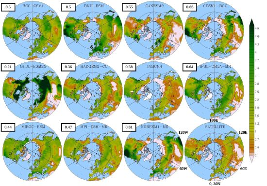
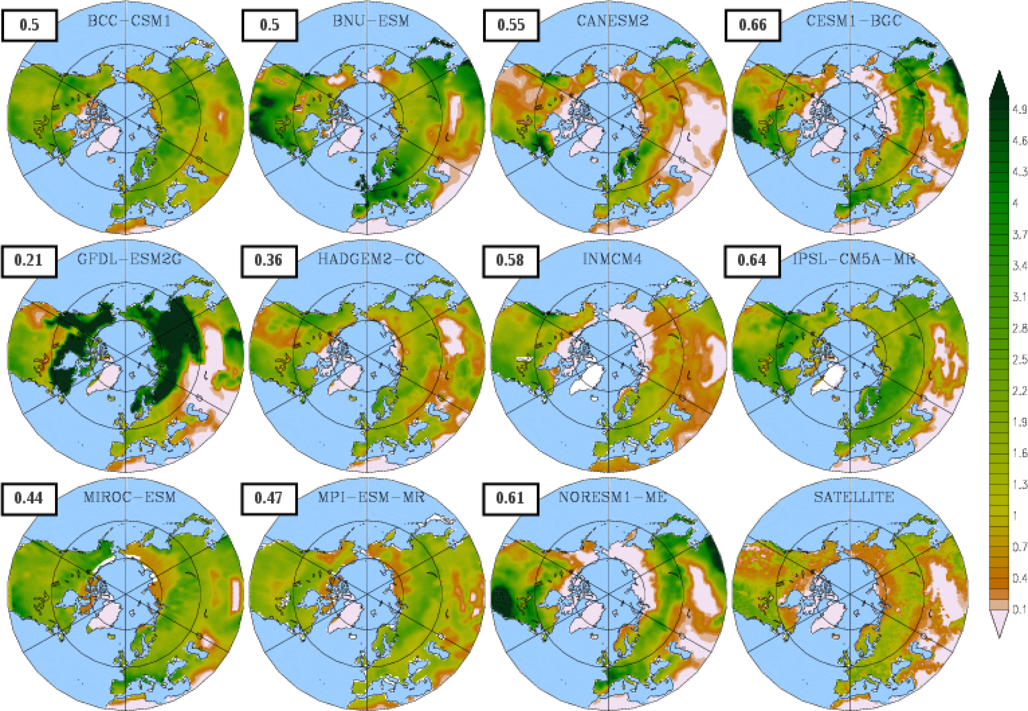
3.1. Mean Leaf Area Index (LAI)
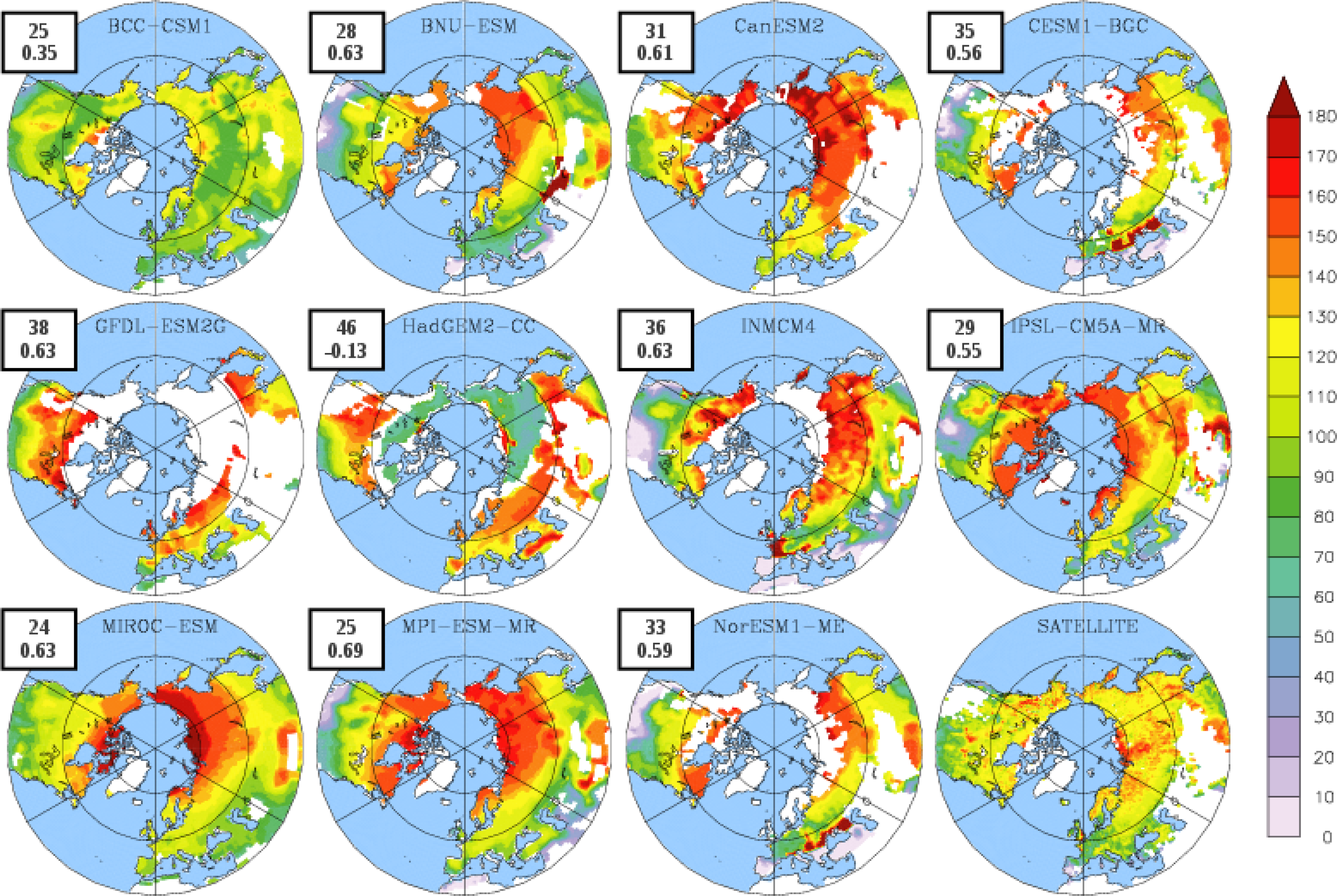
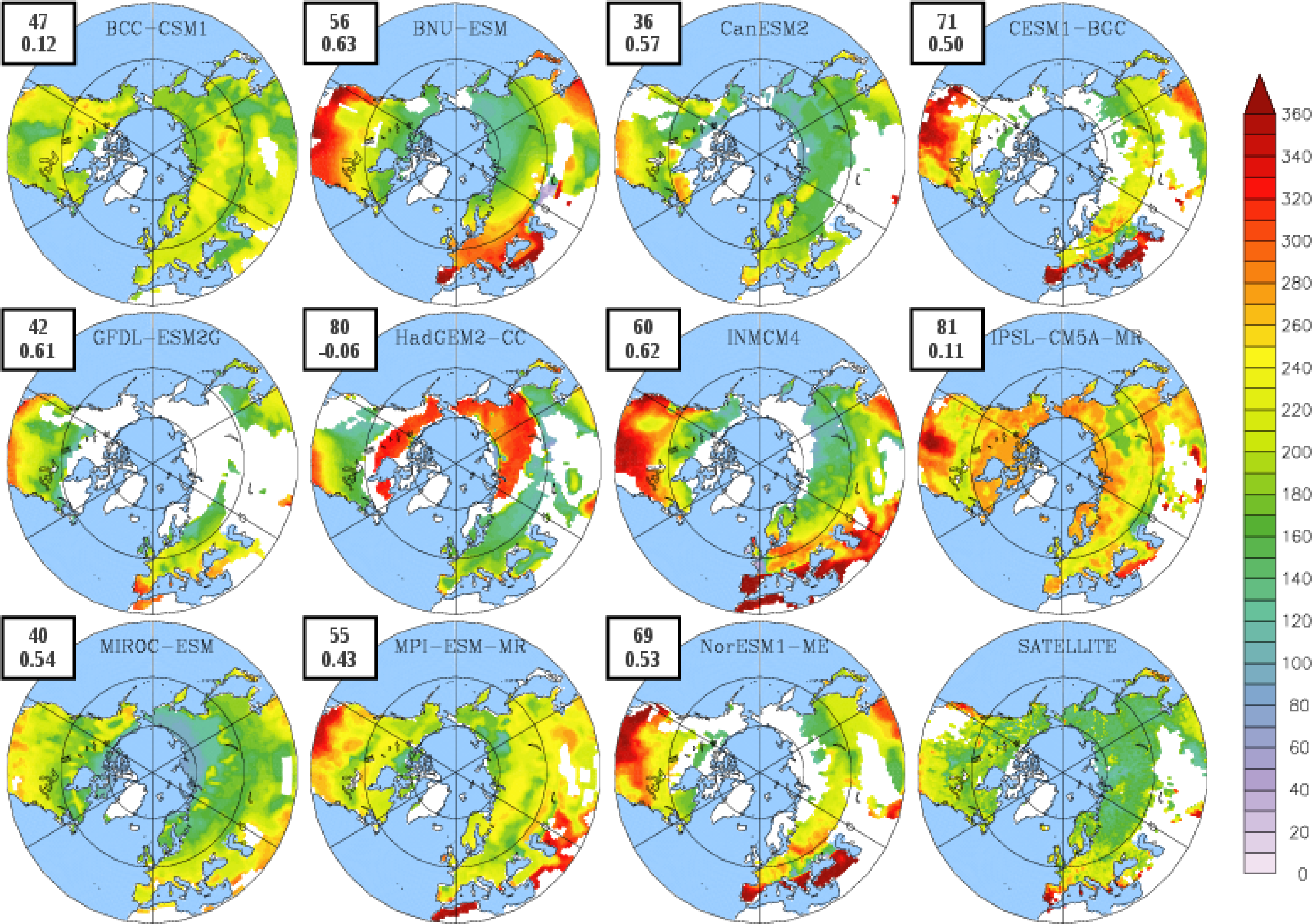
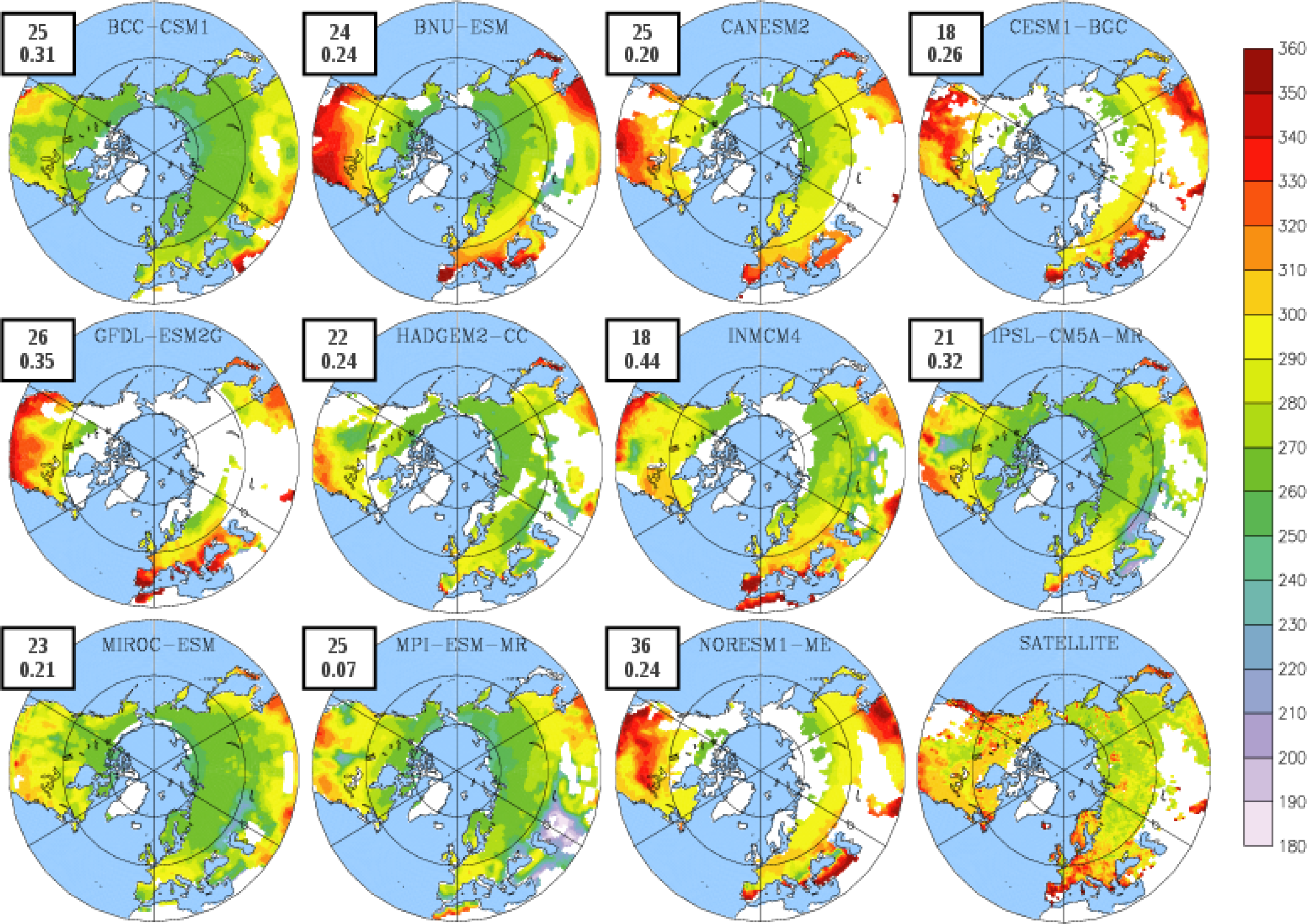
In Figure 1 we present the mean annual LAI (upper panel), the mean annual land precipitation (middle panel), and the mean annual surface temperature (bottom panel) for each model for the period 1986–2005, with the corresponding interannual variability (IAV) and trends. Considering the x-axis of the temperature, models falling at the left of observations (CRU, [89]) indicate a cold bias while models at the right of the reference data have a warm bias. On the y-axis models above the observations have a stronger trend than observations, while the models below the reference value show a lower trend. The same consideration is also valid for the precipitation, namely models falling at the left of observations (CRU) indicate a dry bias (wet bias when falling at the right), while on the y axis models below the observations have a stronger drying trend than observations.
It should also be noted that, to be consistent with LAI, we show the precipitation and temperature only over the land points of the Northern Hemisphere. Finally, we selected CRU as reference data for the validation of climatic variables since it has been used as input data in the offline simulations [90].
The evaluation of the simulated precipitation and temperature is needed to assess whether any bias in the simulated LAI can be related to poor performance of the ESMs at reproducing physical variables, or is mainly due to the poor representation of some biogeochemical processes in the land surface models of ESMs.
Looking at the LAI (Figure 1), in general, except CanESM2 and INMCM4, all the models overestimate the mean annual LAI over the Northern Hemisphere. The poorest performance has been found in GFDL-EMS2G, which shows a mean value of 2.7, much larger than the reference value (0.83); all the other models show a mean annual LAI ranging from 1.2 and 1.7. Conversely, the trends are well captured by quite a few models; specifically, many models are clustered around the reference value, and, according to the observations, all the models show a greening in the last 20 years. The only far outlier is BNU-ESM, having a positive trend 6 times larger than the observed value. The interannual variability is in general well captured by most of the models, although an overestimation of the year-to-year variability is found for a few models; the exceptions are CanESM2 and MPI-ESM-MR, which show an interannual variability slightly lower than LAI3g. Also, in this case, BNU-ESM is the only outlier in reproducing the IAV, having a year-to-year variability much larger than the reference value.
The large bias found in BNU-ESM could be related in some way to the strong wet bias that this model has in reproducing the observed precipitation. Specifically, whilst the mean annual precipitation as reported by CRU data is 520 mm/yr, BNU-ESM shows a mean value of 802 mm/yr. However, it should also be noted that, except CanESM2, all the other models also have a wet bias.
The wet bias found in all the CMIP5 ESM could explain the LAI overestimation: in fact the best agreement between observed and simulated LAI is found for CanEMS2, this being the only model without a wet bias. Although in the boreal and Arctic region the temperature is the main limiting factor for the carbon assimilation, at mid-latitudes the precipitation plays a pivotal role through its control on the soil moisture [91,92].
The precipitation trends in general are well reproduced by the models, being all scattered around the reference data and all showing a wettening over the last 20 years. The exceptions are INMCM4, which does not show any trend in the land precipitation and GFDL-ESM2G, which has a wet bias two times larger than CRU. The interannual variability of the reference data is about 85 mm/yr and only INMCM4, IPSL-CM5A-MR, GFDL-ESM2G and MIROC-ESM well reproduce this value, while CanESM2 (∼80 mm/yr), NorESM1-ME (∼80 mm/yr) and BCC-CSM1 (75 mm/yr) have a slightly lower IAV and the remaining models show a larger IAV. It is noteworthy that MPI-ESM-MR has a IAV two times larger than the reference data.
Looking at the temperature, all the models are clustered around the reference data and only HadGEM2-CC (cold bias) and MIROC-ESM (warm bias) show a bias greater than 1.5 °C. In addition, all the models predict a warming in the Northern Hemisphere during the last 20 years; the weaker trends have been found in HadGEM2-CC and INMCM4 being about 4 times smaller than the one reported by CRU. The observed temperature interannual variability is about 0.8 °C and only INMCM4 and MIROC-ESM have a similar IAV; all the other models show a larger IAV than CRU with NorESM1-ME having an IAV of about 1 °C.
Although models in general show good skills in reproducing the observed climate, we would highlight that this agreement in the mean values over a large region could arise from a compensation between overestimation in some points of the domain and underestimation in other points [85]. This suggests that to perform an exhaustive model validation we should look at the spatial patterns (e.g., maps).
For this reason in Figure 2 we show the spatial distribution of the mean annual LAI in the Northern Hemisphere as calculated from the CMIP5 ESMs and observed by satellite over the period 1986–2005. Results are projected over a stereographic projection from the North Pole, with the latitude ranging from 30°N to 90°N.
The observed spatial pattern of LAI is characterized by a wide maximum over Northern America and by a negative gradient extending from central Europe to Northern-Eastern Asia, with a broad minimum in the Tibetan plateau due to the sparse vegetation. Although there is an overall overestimation by most of the CMIP5 models, 10 out of 11 models correctly reproduce this pattern: in particular CESM1-BGC, IPSL-CM5A-MR, and NorESM1-ME show a very good agreement with observations in terms of locations of the maximum and minimum values, as well as fairly simulating the gradient over the Eurasian region. This is confirmed by the relatively high value (>0.6) of the spatial correlation computed between the models and the reference data. Conversely, GFDL-ESM2G is not able to reproduce this spatial pattern, and LAI values above 5 are simulated over the whole North America and Asia; for this reason this model exhibits the lowest spatial correlation (0.21). It should be noted that, since ESMs generate their own climate, there is no reason to expect models and observations to agree on the phasing of interannual variations [85]; for this reason we did not account the RMSE for the mean annual LAI.
The seasonal amplitude patterns show large disagreement between the models and the satellite data (Figure 3). Some models (e.g., BNU-ESM and MIROC-ESM) clearly overestimate the mean amplitude, which is particularly evident over the whole North America and Eurasia. Other models (e.g., CESM1-BGC, HadGEM2-CC, MPI-ESM-MR, and NorESM1-ME) show a smaller seasonality than satellite data, while INMCM4, CanESM2 and BCC-CSM1 perform better than the rest of the models in reproducing the satellite-derived observations. The RMSE, indicating the mean error of the models in reproducing a given variable, suggests that CanESM2 has the lowest error: in fact this model, albeit it slightly underestimates the seasonal amplitude over the Russia, has the correct magnitude for the observed seasonal amplitude. The same considerations are also valid for IPSL-CM5A-MR, INMCM4 and BCC-CSM1 which show a RMSE of 1.1. Conversely, BNU-ESM and MIROC-ESM show a larger seasonal amplitude than the satellite data, therefore they have high RMSE values.
The spatial correlation, indicating how well models reproduce the observed spatial pattern, confirm that CanESM2, INMCM4 overperform the spatial pattern of the seasonal amplitude compared to other models.

3.2. Growing Season

Figure 4 displays the spatial distribution of the mean onset dates of green-up as calculated from the CMIP5 ESMs and satellite observation for the period 1986–2005. As expected the satellite data show that the mean green-up date is progressively delayed with increasing latitude and increasing continentally [93]. The latest dates of green-up occur in northern Siberia, northern Canada, and over the Tibetan Plateau, owing to low temperatures.
The growing season onset derived from CMIP5 ESMs shows that quite a few models do correctly reproduce the observed spatial pattern, as confirmed by the relatively high spatial correlation (>0.5). The exceptions are BCC-CSM1 who has some patchy areas of agreement with satellite data and HadGEM2-CC who has an earlier onset in the whole Arctic area than in the temperate regions. In the latter case, the wrong pattern leads also to a negative correlation (−0.13).
The models that correctly reproduce the green-up spatial pattern show an overestimation of the onset day, namely these models generally predict later onset values, particularly over the boreal forests of Siberia and Northern America. This leads to the large RMSE values found for the onset in most of the models, ranging from 24 to 38 days.
Considering GFDL-ESM2G, this model shows a larger onset date in the few “non-masked” grid points (Figure 4), while a large area of Eurasia and Northern America shows a seasonal amplitude less than 0.5 (Figure 3). This suggests a problem in the initialization of the vegetation during the spin up phase: in fact the GFDL land model only allows coniferous trees to grow in cold climates, i.e., deciduous trees and grass do not grow in these cold regions. As a result, coniferous trees are established in areas where there should be tundra or cold deciduous trees, and therefore the seasonal amplitude is lower than expected.
Satellite data shows that the dates of vegetation dormancy (Figure 5) occur in reverse order of the green-up onset, namely the green-up wave progresses northwards and dormancy wave progresses southwards [93]. Considering all the 11 ESMs only BNU-ESM, INMCM4, GFDL-ESM2G, and CanESM2 have a dormancy distribution similar to the observed pattern, the spatial correlation being larger than 0.4. The remaining models have some patchy area of agreement, mainly over Europe and the temperate region of North America, while we found relevant problems over the whole Arctic area in HadGEM2-CC, IPSL-CM5A-MR and MPI-ESM-MR, with an offset occurring after DOY 365.
In these regions, where the dominant vegetation is composed by boreal deciduous forest, modelled dormancy can happen after the end of the year (DOY higher than 365). However, the snow corrupts the satellite signal in those months and this partially explains why the errors are large in the dormancy date.
This is particularly evident in IPSL-CM5A-MR that shows a dormancy date around February–March of the new year over the whole Arctic area, while satellite data shows that the offset occurs 5–6 months before. This explains the large RMSE (82 days) found in this model.
Although MIROC-ESM does not show the highest spatial correlation due to a few area of disagreement mainly located in Alaska, it shows one of the lower RMSE (27 days); the other models have errors ranging between 26 days (BCC-CSM1) and almost 3 months (IPSL-CM5A-MR). Compared to other CMIP5 models, GFDL-ESM2G has a smaller RMSE than the average. However it should be noted that it has been computed considering only a few grid points, due to the incorrect representation of the seasonal amplitude.
Looking at the satellite data, the growing season length (Figure 6) is found to increase dramatically with decreasing latitude [93]. It is the shortest in central and eastern Siberia along the Arctic coast, with a duration of only 4 months. In contrast, most of Europe, Eastern China and Southern North America have long growing seasons. The growing season length shows a good agreement between satellite data and models, although individual models like IPSL-CM5A-MR, and HadGEM2-CC still exhibit large errors in reproducing the observed spatial pattern.
Specifically, the best results are found in BNU-ESM, INMCM4, being the correlation systematically greater than 0.6. Besides, in the few grid points covered by deciduous forests GFDL-ESM2G shows a good agreement with satellite GSL and this explains the relative high correlation and low RMSE compared to other ESMs. Consistent with previous results, HadGEM2-CC shows a negative correlation, indicating the inability of this model to reproduce the observed spatial variability. In addition HadGEM2-CC and IPSL-CM5A-MR also show the highest RMSE for the GSL, the error being more than 2 times larger than the lowest RMSE found in CanESM2.

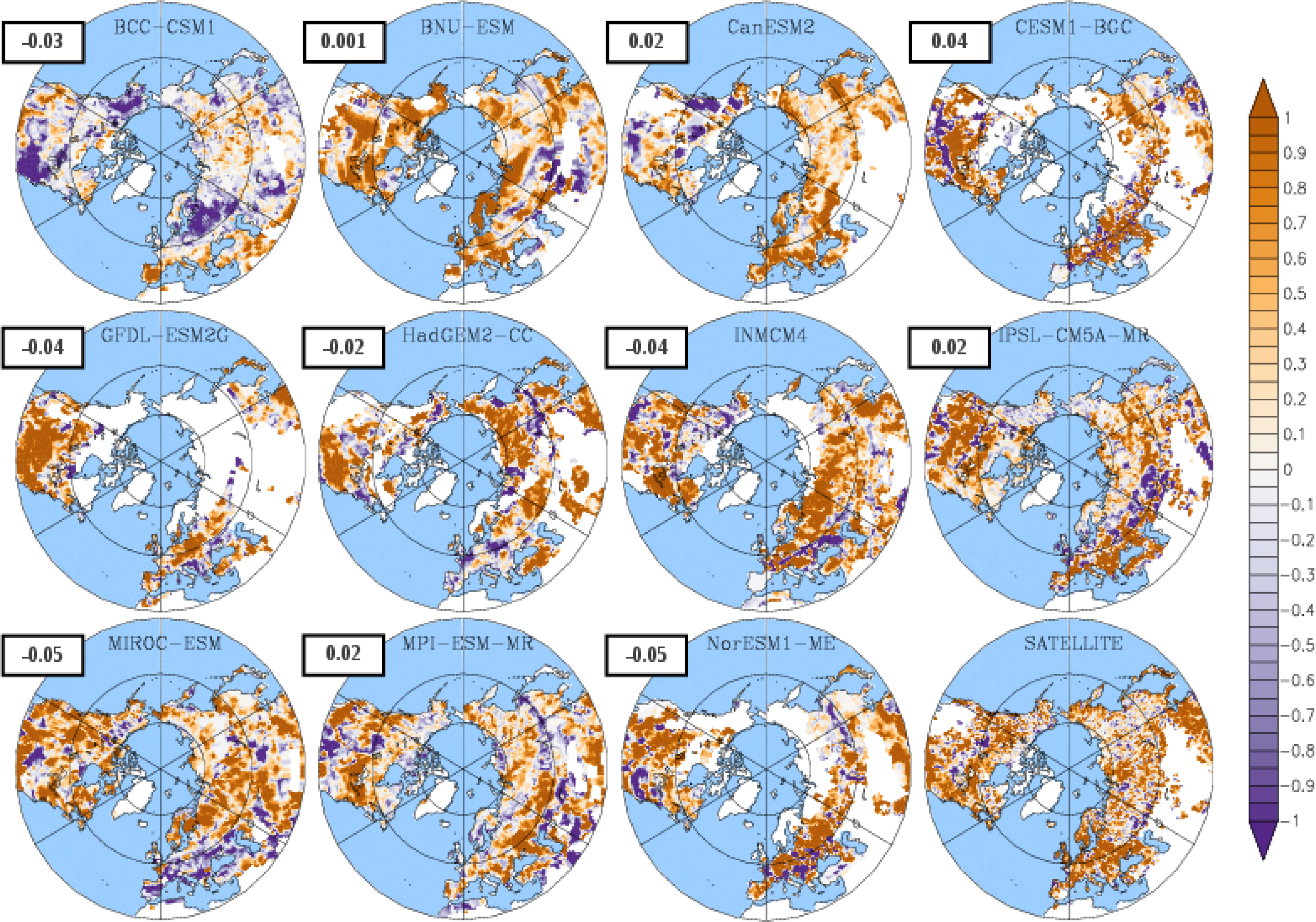
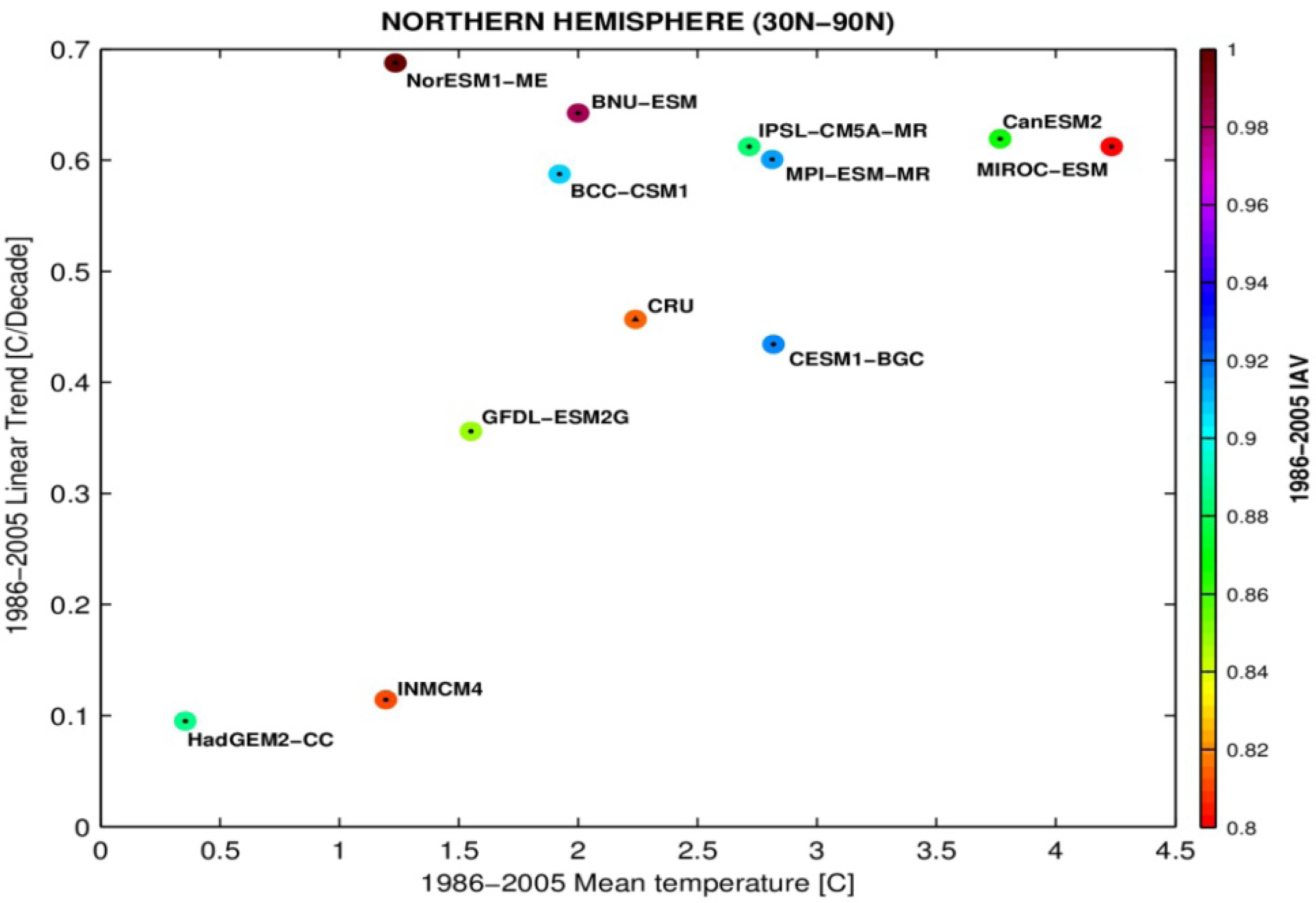
3.3. Temporal Trends

Quite a few models predict an overall increase of LAI with time in most of the Northern Hemisphere, which is consistent with the satellite observations (Figure 7) which show a greening over the whole Eurasia and almost no negative trend in the whole Northern Hemisphere, with a small exception over western North America and few locations in the Eurasian boreal forest.
From the whole compendium, BNU-ESM, GFDL-ESM2G, HadGEM2-CC and NorESM1-ME display the highest increase in LAI (see also Figure 1), mostly over the eastern coast of North America, Europe and the boreal forest of Asia. IPSL-CM5A-MR, MIROC-ESM, BCC-CSM1 and INMCM4 have an intermediate signal with the increase shown over the same regions, and some patchy areas where LAI decreased. We found that none of the models were able to reproduce the correct spatial pattern, the spatial correlation being close to 0 for almost all the models, except MIROC-ESM, which shows a positive correlation of 0.15.
The models also show a general increase in the growing season length, with patchy areas where it decreases (Figure 8). It is clear that from the 11 ESMs, those that perform better at calculating the growing season (both on the onset and dormancy) and LAI also do better for the trends, despite there being no spatial correlation between CMIP5 models and satellite data.

4. Discussion

Results show that all coupled models correctly reproduce the spatial pattern of LAI (Figure 2), although an overall overestimation is found (Figure 1). GFDL-ESM2G clearly shows a strong overestimation over the Northern Hemisphere. Such overestimation in boreal forest is related to the substitution of tundra with coniferous forests; this result is supported by the low seasonal amplitude found over the whole Northern region of Eurasia.
Table 2 reports the comparison of simulated LAI and the leaf phenology, averaged over the whole domain of interest, against satellite observations.
Looking at Table 2, it is clear that all the models overestimate not only the average LAI (except CanESM2), but also the mean dormancy and length of the growing season (except CanESM2 and MIROC-ESM), while the onset shows much agreement between model means and observations (Table 2). Satellite LAI average for the Northern Hemisphere is 0.83 while LAI from the models varies between 0.8 to 2.7. Growing season onset was earlier in 5 out of 11 models, while dormancy came between 9 to 75 days later in the models.
However, when the dormancy period is calculated based on the Gross Primary Production (GPP) the modelled values become much closer to the satellite values, with an average offset occurring at 287 ± 13 days, very similar to the 295 days from the satellite data. In addition, the RMSE shows a noticeable decrease when compared to results of Figure 5. Besides, looking at the spatial pattern, when the offset is computed using the GPP instead of the LAI, all the models show a geographical distribution very similar to the observations (Figure 9). This is confirmed by an increase in the spatial correlations found in 7 out of 11 models compared to results of Figure 5. These results suggest that the leaves in the models remain for longer than they should (discussed later).
Although the wet bias found in most of the analysed CMIP5 models could explain the positive bias in LAI, this overestimation of the mean LAI is consistent with results from the uncoupled models (Table 3), suggesting that it is unlikely that differences in climate in the coupled models are solely responsible for this positive bias. This general overestimation could also be explained by a combination of underestimation of observed LAI, likely due to a saturation of satellite instrumentation, particularly on areas with dense vegetation, and by missing parameterizations of disturbances in the models (e.g., pollution, insect attack, nutrient limitation, grazing, fire dynamics), which leads to a larger amount of carbon stored in the biomass, which, in turn, leads to a larger LAI. The combination of these two effects explains why we found a relevant overestimation of simulated LAI in both coupled and uncoupled models.
The geographical pattern of average LAI is also similar between coupled and uncoupled models [73]. The overestimation of LAI is found consistently over the boreal forest (55°N) when compared to the satellite observations, with better agreement over areas with scarce vegetation. When comparing models with the same vegetation model (TRIFFID vs. HADGEM2-CC, ORCHIDEE vs. IPSL-CM5A-MR and CLM vs. NorESM1 or CESM1-BGC) there are little differences in the distribution of LAI, suggesting that climatic variations in the coupled models are less important in controlling the distribution of LAI than having the correct vegetation distribution and parameterizations.
The onset patterns are similar among all coupled and uncoupled models, with the latest onset occurring over the boreal region. The similarities are even stronger over the dormancy where all models display a general overestimation over the boreal region, possibly explained by the late leaf shed in all models [94].
These results suggest that both coupled and uncoupled models predict a later dormancy (day) and a longer growing season length in comparison to satellite observation (Table 3). It seems that leaves in the models remain for longer than they should. However the late dormancy is not in line with the vegetation photosynthetic activity: in fact, when the same methodology to calculate the end of the photosynthetic active period was applied to the gross primary productivity (GPP), we found that the dormancy began at 277 ± 7 days in the uncoupled models and 287 ± 13 days in case of CMIP5 models, which is remarkably earlier than previously predicted by LAI, and much closer to the observed value of 295 days. It is evident that all models are keeping inactive leaves for longer than they should, which does not have any impact on the carbon cycle but could potentially modify surface radiation budget and turbulent fluxes, affecting therefore the PBL dynamics, which in turn could lead to potential bias in lower atmospheric dynamics simulated by ESMs. In addition to those ESMs having an interactive tropospheric chemistry component, the presence of inactive leaves could modify the deposition fluxes that strongly depend on the area of the canopy [11]. Conversely, the longer offset simulated by offline models does not affect simulation results since the climate is provided as input data and the feedbacks between the land surface and the atmosphere are not taken into account.
Looking at the LAI trends, all the coupled models show a clear greening over the whole Northern America and Eurasia, consistent with satellite data, while not all the offline models show the same pattern over the high latitudes of the Northern Hemisphere. Considering all the ESMs, the greening of the high latitudes is likely driven by positive temperature trend (Figure 1) but in some of the offline models we observe a browning over the same region, suggesting that offline modelled LAI is also sensitive to moisture changes, as most of the browning occurs over areas where precipitation shows a decrease (not shown).
The previous similarities between coupled and uncoupled models, similar geographical distribution of LAI with higher values than the satellite data, and an extended growing season mostly driven by a later dormancy all suggests that the correct initialization, distribution, and parameterization of vegetation in the models is the most important feature in the correct representation of LAI. Nevertheless climatic variables, temperature in particular, have proven to be the main drivers of changes over time [95].

5. Conclusions

We compared LAI as simulated by 11 Earth-System Models against satellite data and uncoupled models [73], for the Northern Hemisphere during the 1986–2005 period. We compared the mean annual LAI, the spatial pattern of LAI and the onset, dormancy and length of the growing season. Our results show that models consistently overestimate the mean value of LAI, although considering the error of the reference data estimated by comparing the satellite data with ground measurements the model-data misfit is significantly reduced. In addition models have an increased growing season, mostly due to a later dormancy, compared to the satellite data. This is consistent with the finding on the uncoupled models.
We conclude that validating LAI in each model against satellite observations should be a fundamental step for all modelling groups. This is essential since LAI is a fundamental variable in all models, required to correctly calculate the hydrological, energetic and carbon fluxes.

Acknowledgments

We acknowledge the World Climate Research Programme’s Working Group on Coupled Modelling, which is responsible for CMIP, and we thank the climate modeling groups (listed in Table 1 of this paper) for producing and making available their model output. For CMIP the US Department of Energy’s Program for Climate Model Diagnosis and Intercomparison provides coordinating support and led development of software infrastructure in partnership with the Global Organization for Earth System Science Portals. We also thank Ranga Myneni for his valuable contribution and comments on the development of the paper, Xuhui Wang for his help on the methodology, and the four anonymous reviewers who helped to improve the paper.
This work was funded by the European Commission’s 7th Framework Programme under Grant Agreements number 238366 (GREENCYCLESII project) and 282672 (EMBRACE project).

Conflict of Interest

The authors declare no conflict of interest.

References and Notes

  1. Myneni, R.B.; Hoffman, S.; Knyazikhin, Y.; Privette, J.L.; Glassy, J.; Tian, Y.; Wang, Y.; Song, X.; Zhang, Y.; Smith, G.; et al. Global products of vegetation leaf area and fraction absorbed PAR from year one of MODIS data. Remote Sens. Environ 2002, 83, 214–231. [Google Scholar]
  2. Sellers, P.J.; Randall, D.A.; Betts, A.K.; Hall, F.G.; Berry, J.A.; Collatz, G.J.; Denning, A.S.; Mooney, H.A.; Nobre, C.A.; Sato, N.; et al. Modeling the exchanges of energy, water, and carbon between continents and the atmosphere. Science 1997, 275, 502–509. [Google Scholar]
  3. Botta, A.; Viovy, N.; Ciais, P.; Friedlingstein, P. A global prognostic scheme of leaf onset using satellite data. Glob. Change Biol 2000, 6, 709–726. [Google Scholar]
  4. Pielke, R.A.; Avissar, R.; Raupach, M.; Dolman, A.J.; Zeng, X.; Denning, A.S. Interactions between the atmosphere and terrestrial ecosystems: Influence on weather and climate. Glob. Change Biol 1998, 4, 461–475. [Google Scholar]
  5. Brovkin, V. Climate-vegetation interaction. J. Phys 2002, 4, 57–72. [Google Scholar]
  6. Chase, T.N.; Pielke, R.; Kittel, T.; Nemani, R.; Running, S. Sensitivity of a general circulation model to global changes in leaf area index. J. Geophys. Res 1996, 101, 7393–7408. [Google Scholar]
  7. Betts, R.A.; Cox, P.M.; Lee, S.E.; Woodward, F.I. Contrasting physiological and structural vegetation feedback in climate change simulations. Nature 1997, 387, 796–799. [Google Scholar]
  8. Piao, S.; Friedlingstein, P.; Ciais, P.; Viovy, N.; Demarty, J. Growing season extension and its impact on terrestrial carbon cycle in the Northern Hemisphere over the past 2 decades. Glob. Biogeochem. Cy 2007, 21, GB3018. [Google Scholar]
  9. Guenther, A.; Karl, T.; Harley, P.; Wiedinmyer, C.; Palmer, P.I.; Geron, C. Estimates of global terrestrial isoprene emissions using MEGAN (Model of Emissions of Gases and Aerosols from Nature). Atmos. Chem. Phys 2006, 6, 3181–3210. [Google Scholar]
  10. Lathière, J.; Hauglustaine, D.A.; Friend, A.D.; De Noblet-Ducoudré, N.; Viovy, N.; Folberth, G.A. Impact of climate variability and land use changes on global biogenic volatile organic compound emissions. Atmos. Chem. Phys 2006, 6, 2129–2146. [Google Scholar]
  11. Petroff, A.; Mailliat, A.; Amielh, M.; Anselmet, F. Aerosol dry deposition on vegetative canopies. Part 1: Review of present knowledge. Atmos. Environ 2008, 42, 3625–3653. [Google Scholar]
  12. Anav, A.; Menut, L.; Khvorostyanov, D.; Viovy, N. A comparison of two canopy conductance parameterizations to quantify the interactions between surface ozone and vegetation over Europe. J. Geophys. Res 2012, 117, G03027. [Google Scholar]
  13. Menzel, A.; Fabian, P. Growing season extended in Europe. Nature 1999, 397, 659. [Google Scholar]
  14. Ahas, R.; Jaagus, J.; Aasa, A. The phenological calendar of Estonia and its correlation with mean air temperature. Int. J. Biometeorol 2000, 44, 159–166. [Google Scholar]
  15. Myneni, R.B.; Keeling, C.D.; Tucker, C.J.; Asrar, G.; Nemani, R.R. Increased plant growth in the northern latitudes from 1981–1991. Nature 1997, 386, 698–702. [Google Scholar]
  16. Zhou, L.; Tucker, C.J.; Kaufmann, R.K.; Slayback, D.; Shabanov, N.V.; Myneni, R.B. Variations in northern vegetation activity inferred from satellite data of vegetation index during 1981 to 1999. J. Geophys. Res 2001, 106, 20069–20083. [Google Scholar]
  17. Tucker, C.J.; Slayback, D.; Pinzon, J.E.; Los, S.O.; Myneni, R.B.; Taylor, M.G. Higher northern latitude normalized difference vegetation index and growing season trends from 1982 to 1999. Int. J. Biometeorol 2001, 45, 184–190. [Google Scholar]
  18. Suzuki, R.; Nomaki, T.; Yasunari, T. West-east contrast of phenology and climate in northern Asia revealed using a remotely sensed vegetation index. Int. J. Remote Sens 2003, 47, 126–138. [Google Scholar]
  19. Stöckli, R.; Vidale, P.L. European plant phenology and climate as seen in a 20-year AVHRR land-surface parameter dataset. Int. J. Remote Sens 2004, 25, 3303–3330. [Google Scholar]
  20. Keeling, C.D.; Chin, J.F.S.; Whorf, T.P. Increased activity of northern vegetation in inferred from atmospheric CO2 measurements. Nature 1996, 382, 146–149. [Google Scholar]
  21. Lucht, W.; Prentice, I.C.; Myneni, R.B.; Sitch, S.; Friedlingstein, P.; Cramer, W.; Bousquet, P.; Buermann, W.; Smith, B. Climatic control of the high-latitude vegetation greening trend and Pinatubo effect. Science 2002, 296, 1687–1689. [Google Scholar]
  22. Barichivich, J.; Briffa, K.R.; Osborn, T.J.; Melvin, T.M.; Caesar, J. Thermal growing season and timing of biospheric carbon uptake across the Northern Hemisphere. Glob. Biogeochem. Cy 2012, 26, GB4015. [Google Scholar]
  23. Kimball, J.; McDonald, K.; Running, S.; Frolking, S. Satellite radar remote sensing of seasonal growing seasons for boreal and subalpine evergreen forests. Remote Sens. Environ 2004, 90, 243–258. [Google Scholar]
  24. Euskirchen, E.S.; McGuire, A.D.; Kicklighter, D.W.; Zhuang, Q.; Clein, J.S.; Dargaville, R.J.; Dye, D.G.; Kimball, J.S.; McDonald, K.C.; Melillo, J.M.; Romanovsky, V.E.; et al. Importance of recent shifts in soil thermal dynamics on growing season length, productivity, and carbon sequestration in terrestrial high-latitude ecosystems. Glob. Change Biol 2006, 12, 731–750. [Google Scholar]
  25. Linderholm, H. Growing season changes in the last century. Agric. For. Meteorol 2006, 137, 1–14. [Google Scholar]
  26. Churkina, G.; Schimel, D.; Braswell, B.; Xiao, X. Spatial analysis of growing season length control over net ecosystem exchange. Glob. Change Biol 2005, 11, 1777–1787. [Google Scholar]
  27. Richardson, A.D.; Black, T.A.; Ciais, P.; Delbart, N.; Friedl, M.A.; Gobron, N.; Hollinger, D.Y.; Kutsch, W.L.; Longdoz, B.; Luyssaert, S.; et al. Influence of spring and autumn phenological transitions on forest ecosystem productivity. Philos. T. R. Soc. B 2010, 365, 3227–3246. [Google Scholar] [Green Version]
  28. Mao, J.; Shi, X.; Thornton, P.E.; Piao, S.; Wnag, X. Causes of spring vegetation growth trends in the northern mid–high latitudes from 1982 to 2004. Environ. Res. Lett 2012, 7, 014010. [Google Scholar]
  29. Mao, J.; Shi, X.; Thornton, P.E.; Hoffman, F.M.; Zhu, Z.; Myneni, R.B. Global latitudinal-asymmetric vegetation growth trends and their driving mechanisms: 1982–2009. Remote Sens 2013, 5, 1484–1497. [Google Scholar]
  30. Smith, N.V.; Saatchi, S.S.; Randerson, J.T. Trends in high northern latitude soil freeze and thaw cycles from 1988 to 2002. J. Geophys. Res 2004, 109, D12101. [Google Scholar]
  31. Christidis, N.; Stott, P.; Brown, S.; Karoly, D.; Caesar, J. Human contribution to the lengthening of the growing season during 1950–99. J. Clim 2007, 20, 5441–5454. [Google Scholar]
  32. Suni, T.; Berninger, F.; Markkanen, T.; Keronen, P.; Rannik, Ü.; Vesala, T. Interannual variability and timing of growing-season CO2exchange in a boreal forest. J. Geophys. Res 2003. [Google Scholar] [CrossRef]
  33. Hänninen, H.; Tanino, K. Tree seasonality in a warming climate. Trends Plant Sci 2011, 16, 412–416. [Google Scholar]
  34. Charney, J.; Quirk, W.J.; Chow, S.-H.; Kornfield, J. A comparative study of the effects of albedo change on drought in semi-arid regions. J. Atmos. Sci 1977, 34, 1366–1385. [Google Scholar]
  35. Sud, Y.C.; Fennessy, M.J. A study of the influence of surface albedo on July circulation in semi-arid regions using the GLAS GCM. J. Climatol 1982, 2, 105–125. [Google Scholar]
  36. Dirmeyer, P.A.; Shukla, J. Albedo as a modulator of climate response to tropical deforestation. J. Geophys. Res 1994, 99, 20863–20877. [Google Scholar]
  37. Shukla, J.; Mintz, Y. Influence of land-surface evapotranspiration on the Earth’s climate. Science 1982, 215, 1498–1501. [Google Scholar]
  38. Douville, H.; Chauvin, F.; Broqua, H. Influence of soil moisture on the Asian and African monsoons. Part I: Mean monsoon and daily precipitation. J. Climate 2001, 14, 2381–2403. [Google Scholar]
  39. Zampieri, M.; D’Andrea, F.; Vautard, R.; Ciais, P.; de Noblet-Ducoudré, N.; Yiou, P. Hot european summers and the role of soil moisture in the propagation of mediterranean drought. J. Climate 2009, 22, 4747–4758. [Google Scholar]
  40. Sud, Y.C.; Shukla, J.; Mintz, Y. Influence of land surface roughness on atmospheric circulation and precipitation: A sensitivity study with a general circulation model. J. Appl. Meteor 1988, 27, 1036–1054. [Google Scholar]
  41. Bounoua, L.; Collatz, G.J.; Los, S.O.; Sellers, P.J.; Dazlich, D.A.; Tucker, C.J.; Randall, D.A. Sensitivity of climate to changes in NDVI. J. Climate 2000, 13, 2277–2292. [Google Scholar]
  42. Oleson, K.W.; Bonan, G.B. The effects of remotely sensed plant functional type and leaf area index in simulations of boreal forest surface fluxes by the NCAR land surface model. J. Hydrometeor 2000, 1, 431–446. [Google Scholar]
  43. Buermann, W.; Dong, J.; Zeng, X.; Myneni, R.B.; Dickinson, R.E. Evaluation of the utility of satellite-based leaf area index data for climate simulation. J. Climate 2001, 14, 3536–3550. [Google Scholar]
  44. Van den Hurk, B.J.J.M.; Viterbo, P.; Los, S.O. Impact of leaf area index seasonality on the annual land surface evaporation in a global circulation model. J. Geophys. Res 2003, 108, 4191. [Google Scholar]
  45. Tian, Y.; Dickinson, R.E.; Zhou, L.; Myneni, R.B.; Friedl, M.; Chaaf, C.B.; Carroll, M.; Gao, F. Land boundary conditions from MODIS data and consequences for the albedo of a climate model. Geophys. Res. Lett 2004, 31, L05504. [Google Scholar]
  46. Kang, H.-S.; Xue, Y.; Collatz, G.J. Impact assessment of satellite-derived leaf area index datasets using a general circulation model: Seasonal variability. J. Climate 2007, 20, 993–1015. [Google Scholar]
  47. Dickinson, R.E.; Henderson-Sellers, A.; Kennedy, P.J. Biosphere-Atmosphere Transfer Scheme (BATS) Version 1e as Coupled to the NCAR Community Climate Model; NCAR Technical Note, NCAR/TN-387+ STR; National Center for Atmospheric Research: Boulder, CO, USA, 1993. [Google Scholar]
  48. Giorgi, F.; Marinucci, M.R.; Bates, G.T. Development of a second generation regional climate model (RegCM2). I. Boundary-layer and radiative transfer processes. Mon. Wea. Rev 1993, 121, 2794–2813. [Google Scholar]
  49. Schulz, J.-P.; Dümenil, L.; Polcher, J.; Schlosser, C.A.; Xue, Y. Land surface energy and moisture fluxes: Comparing three models. J. Appl. Meteor 1998, 37, 288–307. [Google Scholar]
  50. Lawrence, D.M.; Slingo, J.M. An annual cycle of vegetation in a GCM. Part II: Global impacts on climate and hydrology. Clim. Dyn 2004, 22, 107–122. [Google Scholar]
  51. Stier, P.; Feichter, J.; Kinne, S.; Kloster, S.; Vignati, E.; Wilson, J.; Ganzeveld, L.; Tegen, I.; Werner, M.; Balkanski, Y.; et al. The aerosol-climate model ECHAM5-HAM. Atmos. Chem. Phys 2005, 5, 1125–1156. [Google Scholar]
  52. Hourdin, F.; Musat, I.; Bony, S.; Braconnot, P.; Codron, F.; Dufresne, J.-L.; Fairhead, L.; Filiberti, M.A.; Friedlingstein, P.; Grandpeix, J.-Y.; et al. The LMDZ4 general circulation model: Climate performance and sensitivity to parametrized physics with emphasis on tropical convection. Clim. Dyn 2006, 19, 3445–3482. [Google Scholar]
  53. Foley, J.A.; Prentice, I.C.; Ramankutty, N.; Levis, S.; Pollard, D.; Sitch, S.; Haxeltine, A. An integrated biosphere model of land surface processes, terrestrial carbon balance, and vegetation dynamics. Glob. Biogeochem. Cy 1996, 10, 603–628. [Google Scholar]
  54. Sellers, P.J.; Randall, D.A.; Collatz, G.J.; Berry, J.A.; Field, C.B.; Dazlich, D.A.; Zhang, C.; Collelo, G.D.; Bounoua, L. A revised land surface parameterization (SiB2) for atmospheric GCMs, Part I : Model Formulation. J. Climate 1996, 9, 676–705. [Google Scholar]
  55. Foley, J.A.; Levis, S.; Prentice, I.C.; Pollard, D.; Thompson, S.L. Coupling dynamic models of climate and vegetation. Glob. Change Biol 1998, 4, 561–579. [Google Scholar]
  56. Foley, J.A.; Levis, S.; Costa, M.H.; Cramer, W.; Pollard, D. Incorporating dynamic vegetation cover within global climate models. Ecol. Appl 2000, 10, 1620–1632. [Google Scholar]
  57. Bonan, G.; Levis, S.; Sitch, S.; Vertenstein, M.; Oleson, K.W. A dynamic global vegetation model for use with climate models: Concepts and description of simulated vegetation dynamics. Glob. Change Biol 2003, 9, 1543–1566. [Google Scholar]
  58. Pitman, A.J. The evolution of, and revolution in, land surface schemes designed for climate models. Int. J. Climatol 2003, 23, 479–510. [Google Scholar]
  59. Sitch, S.; Smith, B.; Prentice, I.C.; Arneth, A.; Bondeau, A.; Cramer, W.; Kaplan, J.O.; Levis, S.; Lucht, W.; Sykes, M.T.; et al. Evaluation of ecosystem dynamics, plant geography and terrestrial carbon cycling in the LPJ dynamic global vegetation model. Glob. Change Biol 2003, 9, 161–185. [Google Scholar]
  60. Krinner, G.; Viovy, N.; de Noblet-Ducoudré, N.; Ogée, J.; Polcher, J.; Friedlingstein, P.; Ciais, P.; Sitch, S.; Prentice, I.C. A dynamic global vegetation model for studies of the coupled atmosphere-biosphere system. Glob. Biogeochem. Cy 2005, 19, GB1015. [Google Scholar]
  61. Alessandri, A.; Gualdi, S.; Polcher, J.; Navarra, A. Effects of Land Surface-Vegetation on the Boreal Summer Surface Climate of a GCM. J. Climate 2007, 20, 225–278. [Google Scholar]
  62. Taylor, K.; Stouffer, R.; Meehl, G. An overview of CMIP5 and the experiment design. Bull. Am. Meteorol. Soc 2012, 93, 485–498. [Google Scholar]
  63. Collins, W.J.; Bellouin, N.; Doutriaux-Boucher, M.; Gedney, N.; Halloran, P.; Hinton, T.; Hughes, J.; Jones, C.D.; Joshi, M.; Liddicoat, S.; et al. Development and evaluation of an Earth-System model—HadGEM2. Geosci. Model Dev 2011, 4, 1051–1075. [Google Scholar]
  64. Charlson, R.J.; Lovelock, J.E.; Andreae, M.O.; Warren, S.G. Oceanic phytoplankton, atmospheric sulphur, cloud albedo and climate. Nature 1987, 326, 655–661. [Google Scholar]
  65. Cox, P.M.; Betts, R.A.; Jones, C.D.; Spall, S.A.; Totterdell, I.J. Acceleration of global warming due to carbon-cycle feedbacks in a coupled climate model. Nature 2000, 408, 184–187. [Google Scholar]
  66. Rea, J.; Ashley, M. Phenological evaluations using Landsat-1 sensors. Int. J. Biometeorol 1976, 20, 240–248. [Google Scholar]
  67. Girard, C.M. Estimation of phenological stages and physiological states of grasslands from remote-sensing data. Vegetatio 1982, 48, 219–226. [Google Scholar]
  68. White, M.A.; Thornton, P.E.; Running, S.W. A continental phenology model for monitoring vegetation responses to interannual climatic variability. Glob. Biogeochem. Cy 1997, 11, 217–234. [Google Scholar]
  69. Zhang, X.; Friedl, M.A.; Schaaf, C.B.; Strahler, A.H.; Hodges, J.C.F.; Gao, F.; Reed, B.C.; Huete, A. Monitoring vegetation phenology using MODIS. Remote Sens. Environ 2003, 84, 471–475. [Google Scholar]
  70. Zhou, L.; Kaufmann, R.K.; Tian, Y.; Myneni, R.B.; Tucker, C.J. Relation between interannual variations in satellite measures of northern forest greeness and climate between 1982 and 1999. J. Geophys. Res 2003, 108, 4004. [Google Scholar]
  71. Zhang, P.; Anderson, B.; Barlow, M.; Tan, B.; Myneni, R.B. Climate-related vegetation characteristics derived from Moderate Resolution Imaging Spectroradiometer (MODIS) leaf area index and normalized difference vegetation index. J. Geophys. Res 2004, 109, D20105. [Google Scholar]
  72. Ahl, D.E.; Gower, S.T.; Burrows, S.N.; Shabanov, N.V.; Myneni, R.B.; Knyazikhin, Y. Monitoring spring canopy phenology of a deciduous broadleaf forest using MODIS. Remote Sens. Environ 2006, 104, 88–95. [Google Scholar]
  73. Murray-Tortarolo, G.; Anav, A.; Friedlingstein, P.; Sitch, S.; Piao, S.; Zhu, Z. Evaluation of DGVMs in reproducing satellite derived LAI over the Northern Hemisphere. Part I: Uncoupled DGVMs. Remote Sens. 2013. submitted. [Google Scholar]
  74. Earth System Grid Federation (ESGF). Available online: http://pcmdi9.llnl.gov/esgf-web-fe/ (accessed on 1 June 2013).
  75. Wu, T.; Li, W.; Ji, J.; Xin, X.; Li, L.; Wang, Z.; Zhang, Y.; Li, J.; Zhang, F.; Wei, M.; Shi, X.; et al. Global carbon budgets simulated by the beijing climate center climate system model for the last century. J. Geophys. Res. 2013. [Google Scholar] [CrossRef]
  76. BNU-ESM. Available online: http://esg.bnu.edu.cn/BNU_ESM_webs/htmls/index.html (accessed on 1 June 2013).
  77. Arora, V.K.; Scinocca, J.F.; Boer, G.J.; Christian, J.R.; Denman, K.L.; Flato, G.M.; Kharin, V.V.; Lee, W.G.; Merryfield, W.J. Carbon emission limits required to satisfy future representative concentration pathways of greenhouse gases. Geophys. Res. Lett 2011, 38, L0580. [Google Scholar]
  78. Lindsay, K.; Bonan, G.B.; Doney, S.C.; Hoffman, F.M.; Lawrence, D.M.; Long, M.C.; Mahowald, N.M.; Moore, J.K.; Randerston, J.T.; Thornton, P.E. Preindustrial control and 20th century carbon cycle experiments with the earth system model CESM1-(BGC). J. Climate 2013. submitted. [Google Scholar]
  79. Dunne, J.P.; John, J.G.; Shevliakova, E.; Stouffer, R.J.; Krasting, J.P.; Malyshev, S.L.; Milly, P.C.D.; Sentman, L.T.; Adcroft, A.J.; Cooke, W.; et al. GFDL’s ESM2 global coupled climate-carbon Earth system models. Part II: Carbon system formation and baseline simulation characteristics. J Climate 2013, 26, 2247–2267. [Google Scholar]
  80. Volodin, E.M.; Dianskii, N.A.; Gusev, A.V. Simulating present day climate with the INMCM4.0 coupled model of the atmospheric and oceanic general circulations. Izv. Ocean. Atmos. Phys 2010, 46, 414–431. [Google Scholar]
  81. Dufresne, J.-L.; Foujols, M.-A.; Denvil, S.; Caubel, A.; Marti, O.; Aumont, O.; Balkanski, Y.; Bekki, S.; Bellenger, H.; Benshila, R.; et al. Climate change projections using the IPSL-CM5 Earth system model: From CMIP3 to CMIP5. Clim. Dyn 2013, 40, 2123–2165. [Google Scholar]
  82. Watanabe, S.; Hajima, T.; Sudo, K.; Nagashima, T.; Takemura, T.; Okajima, H.; Nozawa, T.; Kawase, H.; Abe, M.; Yokohata, T.; et al. MIROC-ESM 2010: Model description and basic results of CMIP5–20c3m experiments. Geosci. Model Dev 2011, 4, 845–872. [Google Scholar]
  83. Raddatz, T.; Reick, C.H.; Knorr, W.; Kattge, J.; Roeckner, E.; Schnur, R.; Schnitzler, K.-G.; Wetzel, P.; Jungclaus, J. Will the tropical land biosphere dominate the climate-carbon cycle feedback during the twenty-first century? Clim. Dyn 2007, 29, 565–574. [Google Scholar]
  84. Bentsen, M.; Bethke, I.; Debernard, J.B.; Iversen, T.; Kirkevåg, A.; Seland, Ø.; Drange, H.; Roelandt, C.; Seierstad, I.A.; Hoose, C.; et al. The Norwegian earth system model, NorESM1-M. Part 1: Description and basic evaluation. Geosci. Model Dev. Discuss 2012, 5, 2843–2931. [Google Scholar]
  85. Anav, A.; Friedlingstein, P.; Kidston, M.; Bopp, L.; Ciais, P.; Cox, P.M.; Jones, C.D.; Jung, M.; Myneni, R.B.; Zhu, Z. Evaluating the land and ocean components of the global carbon cycle in the CMIP5 Earth System Models. J Climate 2013, in press. [Google Scholar]
  86. Zhu, Z.; Bi, J.; Pan, Y.; Ganguly, S.; Anav, A.; Xu, L.; Samanta, A.; Piao, S.; Nemani, R.R.; Myneni, R.B. Global data sets of vegetation leaf area index (LAI)3g and Fraction of photosynthetically active radiation (FPAR)3g derived from global inventory modeling and mapping studies (GIMMS) normalized difference vegetation index (NDVI3g) for the period 1981 to 2011. Remote Sens 2013, 5, 927–948. [Google Scholar]
  87. Fang, H.; Jiang, C.; Li, W.; Wei, S.; Baret, F.; Chen, J.M.; Haro, J.G.; Liang, S.; Liu, R.; Myneni, R.B.; et al. Characterization and intercomparison of global moderate resolution leaf area index (LAI) products: Analysis of climatologies and theoretical uncertainties. J. Geophys. Res 2013, 118, 529–548. [Google Scholar]
  88. Zhu, W.; Tian, H.; Xu, X.; Pan, Y.; Chen, G.; Lin, W. Extension of the growing season due to delayed autumn over mid and high latitudes in North America during 1982–2006. Global Ecol. Biogeogr 2012, 21, 260–271. [Google Scholar]
  89. Mitchell, T.D.; Jones, P.D. An improved method of constructing a database of monthly climate observations and associated high-resolution grids. Int. J. Climatol 2005, 25, 693–712. [Google Scholar]
  90. McGuire, A.D.; Christensen, T.R.; Hayes, D.; Heroult, A.; Euskirchen, E.; Yi, Y.; Kimball, J.S.; Koven, C.; Lafleur, P.; Miller, P.A.; et al. An assessment of the carbon balance of arctic tundra: Comparisons among observations, process models, and atmospheric inversions. Biogeosciences 2012, 9, 3185–3204. [Google Scholar]
  91. Nemani, R.R.; Keeling, C.D.; Hashimoto, H.; Jolly, W.M.; Piper, S.C.; Tucker, C.J.; Myneni, R.B.; Running, S.W. Climate-driven increases in global terrestrial net primary production from 1982 to 1999. Science 2003, 300, 1560–1563. [Google Scholar]
  92. Piao, S.; Ciais, P.; Friedlingstein, P.; de Noblet-Ducoudre, N.; Cadule, P.; Viovy, N.; Wang, T. Spatiotemporal patterns of terrestrial carbon cycle during the 20th century. Glob. Biogeochem. Cy 2009, 23, GB4026. [Google Scholar]
  93. Zeng, H.; Jia, G.; Epstein, H. Recent changes in phenology over the northern high latitudes detected from multi-satellite data. Environ. Res. Lett 2011, 6, 045508. [Google Scholar]
  94. Richardson, A.D.; Anderson, R.S.; Arain, M.A.; Barr, A.G.; Bohrer, G.; Chen, G.; Chen, J.M.; Ciais, P.; Davis, K.J.; Desai, A.R.; et al. Terrestrial biosphere models need better representation of vegetation phenology: Results from the North American carbon program site synthesis. Glob. Change Biol 2011, 18, 566–584. [Google Scholar]
  95. Jeong, S.-J.; Ho, C.-H.; Gim, H.J.; Brown, M.E. Phenology shifts at start vs. end of growing season in temperate vegetation over the Northern Hemisphere for the period 1982–2008. Glob. Change Biol 2011, 17, 2385–2399. [Google Scholar]
Figure 1. The x-axis shows the observed and simulated mean annual leaf area index (LAI) (top), annual land precipitation (middle), and mean annual surface temperature over land (bottom). The y-axis shows the temporal trend, while the colorbar reports the interannual variability as computed from the annual standard deviation.
Remotesensing 05 03637f1aRemotesensing 05 03637f1b
Figure 2. Spatial distribution of mean annual leaf area index (LAI) as simulated by 11 Earth System Models (ESMs) and observed by satellite over the period 1986–2005 in the Northern Hemisphere (30°–90°N). The value in the box represents the spatial correlation between modelled and satellite values.
Remotesensing 05 03637f2
Figure 3. Leaf area index (LAI) Seasonal amplitude as simulated by 11 Earth System Models (ESMs) and satellite observations for the Northern Hemisphere (30°–90°N). Spatial correlation and root mean square errors between the respective model and observations are given in the white box.
Remotesensing 05 03637f3
Figure 4. Mean growing season onset (day) as simulated by 11 Earth System Models (ESMs) and satellite observations over the Northern Hemisphere (30°–90°N). For each model we masked out all the grid points where the seasonal amplitude is less than 0.5 (see Figure 3). In the box the value of root mean square error (in days) and spatial correlation, as computed from mean annual data, are presented for each model against the observations.
Remotesensing 05 03637f4
Figure 5. Mean growing season dormancy (day) as simulated by 11 Earth System Models (ESMs) and satellite observations over the Northern Hemisphere (30°–90°N). For each model we masked out all the grid points where the seasonal amplitude is less than 0.5 (see Figure 3). In the box the value of root mean square error (in days) and spatial correlation, as computed from mean annual data, are presented for each model against the observations.
Remotesensing 05 03637f5
Figure 6. Mean growing season length (days) for 11 Earth System Models (ESMs) and satellite observations over the Northern Hemisphere (30°–90°N). For each model we masked out all the grid points where the seasonal amplitude is less than 0.5 (see Figure 3). In the box the value of root mean square error (in days) and spatial correlation, as computed from mean annual data, are presented for each model against the observations.
Remotesensing 05 03637f6
Figure 7. Observed and simulated Leaf Area Index (LAI) trends (%) computed over the period 1986–2005 for 11 Earth System Models (ESMs) and satellite observations over the Northern Hemisphere (30°–90°N). For each model we masked out all the grid points where the seasonal amplitude is less than 0.5 (see Figure 3). The value in the box represents the spatial correlation between modelled and satellite data.
Remotesensing 05 03637f7
Figure 8. Observed and simulated Growing Season Length (GSL) trends (days/year) computed over the period 1986–2005 for 11 CMIP5 ESMs and satellite observations over the Northern Hemisphere (30°–90°N). For each model we masked out all the grid points where the seasonal amplitude is less than 0.5 (see Figure 3). The value in the box represents the spatial correlation between modelled and satellite data.
Remotesensing 05 03637f8
Figure 9. Mean growing season dormancy (day) as simulated by 11 Earth System Models (ESMs) and satellite observations over the Northern Hemisphere (30°–90°N) computed using the Gross Primary Production (GPP). For each model we masked out all the grid points where the Leaf Area Index (LAI) seasonal amplitude is less than 0.5 (see Figure 3). In the box the value of root mean square error (in days) and spatial correlation, as computed from mean annual data, are presented for each model against the observations.
Remotesensing 05 03637f9
Table 1. Coupled Model Intercomparison Project Phase 5 (CMIP5) Earth System Models used in this study with the associated land models and main features controlling the terrestrial carbon cycle.
ModelsSourceLand ModelsDynamic Vegetation#PFTsN CycleResolution (Lat. × Lon.)Reference
BCC-CSM1Beijing Climate Center, ChinaBCC_AVIM1.0N15N∼2.8125° × 2.8125°[75]
BNU-ESMBeijing Normal University, ChinaCoLMYn/aY∼2.8125° × 2.8125°[76]
CanESM2Canadian Centre for Climate Modelling and Analysis, CanadaCLASS2.7 + CTEM1N9N∼2.8125° × 2.8125°[77]
CESM1-BGCNational Center for Atmospheric Research, USACLM4N15Y1.25° × 0.9[78]
GFDL-ESM2GGeophysical Fluid Dynamics Laboratory, USALM3Y5N2° × 2.5°[79]
HadGEM2-CCMet Office Hadley Centre, UKJULES + TRIFFIDY5N1.25° × 1.875°[63]
INMCM4Institute for Numerical Mathematics, RussiaSimple modelNn/aN1.5° × 2[80]
IPSL-CM5A-MRInstitut Pierre Simon Laplace, France Japan Agency for Marine-Earth Science and Technology, Japan;ORCHIDEEN13N1.25° × 2.5°[81]
MIROC-ESMAtmosphere and Ocean Research Institute, Japan;
National Institute for Environmental Studies, Japan
MATSIRO + SEIB-DGVMY13N∼2.8125° × 2.8125°[82]
MPI-ESM-MRMax Planck Institute for Meteorology, GermanyJSBACH + BETHYY12N1.875° × 1.875°[83]
NorESM1-MENorwegian Climate Centre, NorwayCLM4N16Y1.9° × 2.5°[84]
Table 2. Average Leaf Area Index (LAI), onset, dormancy and growing season length average for the Northern Hemisphere for each model and satellite observations. The values for dormancy and length based on Gross Primary Production (GPP) are presented in brackets.
ModelLAIOnsetDormancyLength
BCC-CSM11.54102304 (274)203 (146)
BNU-ESM1.75109323 (280)214 (148)
CanESM20.80140318 (295)178 (149)
CESM1-BGC1.20109343 (305)233 (190)
GFDL-ESM2G2.70131330 (304)199 (152)
HadGEM2-CC1.17115325 (279)210 (132)
INMCM41.00106329 (289)223 (164)
IPSL-CM5A-MR1.68121370 (276)249 (131)
MIROC-ESM1.66124307 (276)183 (130)
MPI-ESM-MR1.35121347 (274)227 (147)
NorESM1-ME1.30109342 (303)219 (186)
LAI3g0.83111295184
Table 3. Comparison of coupled and uncoupled ensemble means of Leaf Area Index (LAI) and phenology averaged over the Northern Hemisphere (30°–90°N).
LAIOnsetDormancyLength
Uncoupled1.55 ± 0.45131 ± 10339 ± 20 (277±7)208 ± 25 (137±20)
Coupled1.47 ± 0.51117 ± 12331 ± 19 (287±13)214 ± 22 (152±20)
LAI3g0.83111295184

