Article

Automatic Removal of Imperfections and Change Detection for Accurate 3D Urban Cartography by Classification and Incremental Updating

by
Ahmad Kamal Aijazi
1,2,
Paul Checchin
1,2,* and
Laurent Trassoudaine
1,2
1
Institut Pascal, Université Blaise Pascal, Clermont Université, BP 10448, F-63000 Clermont-Ferrand, France
2
Institut Pascal, CNRS, UMR 6602, F-63171 Aubière, France
*
Author to whom correspondence should be addressed.
Remote Sens. 2013, 5(8), 3701-3728; https://doi.org/10.3390/rs5083701
Submission received: 27 May 2013 / Revised: 12 July 2013 / Accepted: 16 July 2013 / Published: 30 July 2013
(This article belongs to the Special Issue Advances in Mobile Laser Scanning and Mobile Mapping)

Abstract

:
In this article, we present a new method of automatic 3D urban cartography in which different imperfections are progressively removed by incremental updating, exploiting the concept of multiple passages, using specialized functions. In the proposed method, the 3D point clouds are first classified into three main object classes: permanently static, temporarily static and mobile, using a new point matching technique. The temporarily static and mobile objects are then removed from the 3D point clouds, leaving behind a perforated 3D point cloud of the urban scene. These perforated 3D point clouds obtained from successive passages (in the same place) on different days and at different times are then matched together to complete the 3D urban landscape. The changes occurring in the urban landscape over this period of time are detected and analyzed using cognitive functions of similarity, and the resulting 3D cartography is progressively modified accordingly. The specialized functions introduced help to remove the different imperfections, due to occlusions, misclassifications and different changes occurring in the environment over time, thus ncreasing the robustness of the method. The results, evaluated on real data, demonstrate that not only is the resulting 3D cartography accurate, containing only the exact permanent features free from imperfections, but the method is also suitable for handling large urban scenes.

1. Introduction

In the last few years, automatic 3D urban cartography and modeling have gained immense interest in the scientific community, due to the ever-increasing demand for urban landscape analysis for different popular applications coupled with the recent advances in 3D data acquisition technologies. Integrated in several geographical navigators, like Google Street-Map Viewer, Microsoft Visual Earth or Géoportail, several such models are accessible to a wide public, who enthusiastically view the real-like representation of the urban environment, created by mobile terrestrial data acquisition techniques. However, in urban environments, this task consisting in automatically generating accurate and reliable 3D cartography and models, without imperfections, using the data obtained from these hybrid terrestrial vehicles still remains a challenge. These imperfections mainly include missing features/regions, due to occlusions caused by the presence of temporarily stationary and dynamic objects (pedestrians, cars, etc.) in the scenes [1], false features resulting from misclassifications of objects in the scene [2] and failure to effectively incorporate different changes occurring in the environment over time [3]. In this paper, we present a new method for automatic 3D urban cartography that progressively removes these imperfections in an effective manner.

2. Related Work

The work on handling such imperfections in automatic 3D urban cartography is heavily biased towards occlusion detection and management. Criminisi et al. [4] present a technique of inpainting based on the patch exemplar-based method for completing occluded regions in images. Wang et al. [5] extended this approach to also infer depth from stereo pairs. Wang et al. [6] used a similar method for 3D data, but occlusions were found automatically using object-specific detectors, making it more suitable for larger data sets. Several works have suggested that manual workload can be greatly reduced by using interactive methods that allow a user to quickly mark foreground and background areas, while exact segmentations are determined using graph cuts. In [7], the authors present a Patch-Match algorithm that allows for interactive rates for inpainting and reshuffling via simple user-defined constraints and efficient nearest neighbor search. In the context of building façades and urban reconstruction, increased contextual knowledge is available by assuming the planarity of the structure and the repetition of features, such as floors, windows, etc. Building models are reconstructed by detecting floors and estimating building height in [8]. Occlusions are removed by cloning upper floors and propagating them downward. In [9], multiple views and median fusion are used to remove most occlusions, requiring inpainting only for smaller regions. A method relying on LiDAR point cloud to find and remove occlusions by combining image fusion and inpainting is presented by Benitez et al. [10]. Xiao et al. [11] semantically segmented street-side scenes into several classes, including vegetation and vehicles, but did not actively fill in missing data. Instead, they relied on the missing information being available from other views. In [12,13], two methods for occlusion-free texture generation are presented, but a minimum of three overlapping images is necessary, which requires a high acquisition rate or a very slow driving speed in narrow streets.
A method is discussed in [14], which consists in aligning multiple scans from various viewpoints to ensure the 3D scene model completeness for complex and unstructured underground environments. A technique for extracting features from urban buildings by fusing camera and LiDAR data is discussed in [15], but it does not specifically address this problem and relies on their simple geometrical modeling to complete partially occluded features. Frueh et al. [16] propose a method in which the point cloud is used to generate a 3D mesh that is then classified as foreground or background. Large holes in the background layer, caused by occlusions from foreground layer objects, are then filled by planar or horizontal interpolation. However, such an approach may result in false features in case of insufficient repetitions or lack of symmetry [17]. In our work, we aim to resolve this problem by using a multi-sessional approach in which multiple scans of the same environment obtained on different days and at different times of the day are matched and used to complete the occluded regions.
Automatic detection of changes in urban environment for updating cartography and maps has lately gained some interest in the scientific community. Most of the proposed techniques detect changes in the urban environment from airborne data using Digital Surface Models (DSMs), such as [18,19]. Vögtle and Steinle [2] propose a methodology for detecting changes in urban areas following disastrous events. Instead of solely computing the difference between the laser-based DSMs, a region growing segmentation procedure is used to separate the objects and detect the buildings; only then, an object-based comparison is applied. However, this method remains susceptible to misclassifications. Bouziani et al. [20] presented a knowledge-based change detection method for the detection of demolished and new buildings from very high resolution satellite images. Different object properties, including possible transitions and contextual relationships between object classes, were taken into account. Map data were used to determine processing parameters and to learn object properties. Matikainen et al. [21] also present a change detection method to update building maps, which compares buildings detected by a classification tree method with an existing building map. Some additional rules relying on existing map data are added to handle some likely misclassifications. Unlike these methods, in our work, we handle the 3D point cloud at the 3D grid level for change detection, instead of the object level, making it more robust against misclassifications.
Most of the work using terrestrial laser scans focuses on deformation analysis for designated objects. Change is detected by subtraction of a resampled set of the data [22] or adjustment to surface models, like planes [23] and cylinders [24]. In order to detect changes in large scenes, Hsiao et al. [25] combine terrestrial laser scanning and conventional surveying devices to acquire and register topographic data. The dataset is then transformed into a 2D grid and is compared with information obtained by the digitization of these existing topographic maps.
In [26], changes are detected in the 3D Cartesian world, and the possibilities of scan comparison in point-to-point, point-to-model or model-to-model manners are discussed. The authors then use point-to-point comparison with some adaptations and make use of an octree as a data structure for accessing the 3D point cloud. Comparison is then carried out by using the Hausdorff distance as a measure for changes. Hyyppä et al. [27] also use the method of point-to-point matching for detecting changes in 3D urban scenes. However, due to bad point registration, incorrect corresponding point pairs are likely to cause false change detection. Whereas our method is more robust to such situations, as it not only analyzes the point cloud at the point level, but also at the grid level for this task. Zeibak and Filin [28] extend this method by further characterizing the changes caused by occlusions. Kang et al. [29] not only detect changes in buildings in the urban environment, but also quantify the changed regions using a series of point cloud epochs over time and rebuilt building models. However, this work only focuses on disappearing changes. In our work, we not only detect, but also analyze both appearing and disappearing changes in the 3D urban scene by using 3D evidence grid and cognitive similarity functions.
Algorithm 1. Automatic 3D Urban Cartography
Require: 3D urban point clouds for passage number, np
  • 1: Classify 3D urban point cloud obtained from each of the two sensors into six groups: {road, building, car, pole, tree, unclassified}
  • 2: Compare the classified objects from the two point clouds to further classify them as: {permanently static, temporarily static, mobile} and merge the two point clouds
  • 3: Separate out temporarily static and mobile objects, leaving behind a perforated 3D point cloud, P(np)
  • 4: Store temporarily static objects in a register, R(np)
Sequential update function:{
  • 5: Match and compare P(np) with P(np − 1) to fill in holes and complete 3D cartography }
  • 6: Formulate 3D evidence grids for P(np) and P(np − 1) and compute 3D cell scores, CS, for both
  • 7: Calculate similarity scores, Sym and ASyms, and uncertainty measures for the 3D cells
  • 8: Update similarity map, SMap
Automatic reset function: {
  • 9: Compare the Sym, ASyms and the uncertainty measures of the 3D cells in the SMap after nreset number of passages
  • 10: If there is low Sym and uncertainty measure, then reset those 3D cell(s) in P(np) with those in the recently acquired point cloud (perforated) }
Object update function: {
  • 11: Compare temporarily static objects in R(np) with R(np − 1)
  • 12: Upgrade temporarily static objects in R(np) if they are repeated in nupdate number of passages as permanently static and add in P(np) }
  • 13: Delete 3D evidence grids for P(np) and P(np − 1)
  • 14: Store SMap
  • 15: Update and store R(np)
  • 16: Store P(np)
  • 17: R(np − 1) ← R(np) and P(np − 1) ← P(np)
  • 18: return P(np)
According to the best of our knowledge, no prior work has ever been presented that first effectively detects, then analyzes the changes occurring in the 3D urban scene, in this manner, using terrestrial data and, eventually, updates the 3D cartography accordingly.
Recently, the increasing demand for updated 3D maps and models for different popular applications has prompted frequent scanning of the same urban environment (i.e., multiple passages) using mobile terrestrial data acquisition vehicles. Although these applications utilize the recently acquired scans/data to simply refresh/update the resulting maps and models, they fail to exploit the redundant data available for further use, such as occlusion handling and accurate change detection and updating. Hence, our method successfully takes advantage of the already available redundant data, not only to detect, analyze and update changes in the urban environment, but also to complete occluded regions, so as to ensure that the resulting 3D cartography contains only the exact, actual and permanent features free from imperfections. The proposed method solves the above mentioned problems by handling the point cloud at three different levels using special dedicated functions: (1) the point level to accurately complete occluded regions; (2) the grid level to analyze and handle different changes occurring in the urban environment; and (3) the object level to accommodate for misclassifications and other unclassified objects. In this method, the 3D urban data obtained from mobile terrestrial LiDARs in each passage is directly geo-referenced. These geo-referenced 3D point clouds are segmented and, then, classified into three main object classes: permanently static, temporarily static and mobile. The temporarily static and mobile objects are then removed from the 3D point clouds, which are then merged together, leaving behind a perforated 3D point cloud of the urban scene. These perforated 3D point clouds obtained from different passages (in the same place) on different days and at different times are then matched together to complete the 3D urban landscape. Different changes occurring in the urban landscape over this period of time are studied using cognitive functions of similarity, and the resulting 3D cartography is progressively modified accordingly. An overview of the method is presented in Algorithm 1.

3. 3D Scan Registration

Different features and robust landmarks extracted from 3D images as points of interest and as references for image mapping and scan registrations have commonly been used for different multi-sessional SLAM (Simultaneous Localization And Mapping) algorithms [30]. This approach works well in simple repetitive paths. However, some more complex situations can be found in urban environments, where the selected features/regions can be occluded. When the data acquiring vehicle enters from different directions, then the path is not repetitive. As a result, the selected features/regions may not be readily visible. Thus, in order to cater to this problem, the method of direct geo-referencing of 3D LiDAR points is found most suitable in our case. The method uses integrated GPS/IMUdata to directly orient laser data from its local reference frame to the mapping reference frame (WGS84). The advantage of using this method is that the transformation between the local laser reference frame and the mapping reference frame is known at any given moment (as long as the laser is synchronized), independently, if the laser is collecting data in a static mode or in kinematic mode. Thus, the laser can be used as a push broom sensor sweeping the scene with profiles, while fixing the scan angles as the vehicle moves.
The data that we have used to evaluate our work are the dynamic data set of the 3D Urban Data Challenge 2011, which contains dynamic scenes from downtown Lexington, Kentucky, USA, obtained from the Vis Center’s (University of Kentucky) LiDAR Truck containing two Optech LiDAR sensor heads (high scan frequency up to 200 Hz), a GPS, an inertial measurement unit and a spherical digital camera, as shown in Figure 1.

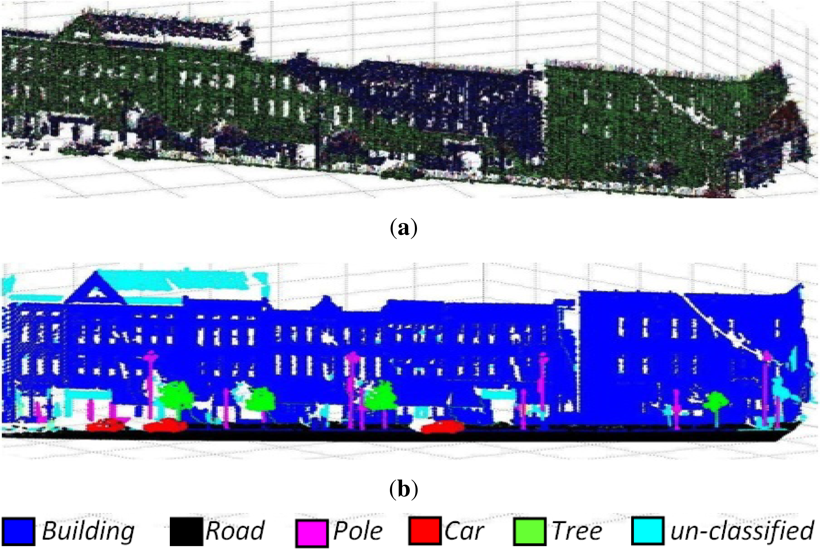
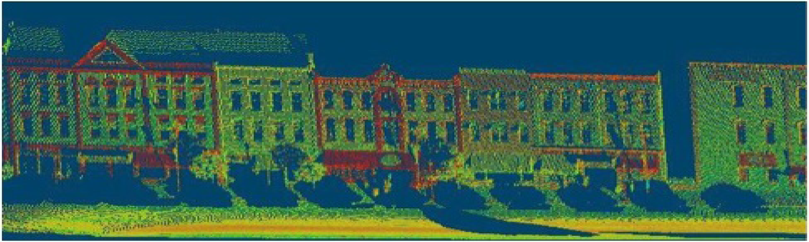
4. Classification of 3D Urban Environment

In urban environments, the quality of the data acquired by different mobile terrestrial data acquisition systems is widely hampered by the presence of temporary static and dynamic objects (pedestrians, cars, etc.) in the scene. As a result, there is a problem of occlusion of regions. Moving objects or certain temporary stationed objects (parked cars, traffic, pedestrian, etc.) present in the area hide certain zones of the urban landscape (buildings, road sides, etc.). Therefore, the first step for 3D urban cartography is to obtain the permanent cartography. This is achieved by removing/extracting the temporarily static and dynamic objects from the scene/point cloud, leaving behind only the permanent features.
In order to achieve this, we classify the urban environment into three main categories: permanently static objects, temporarily static objects and mobile objects. In order to achieve this goal, the 3D point cloud is first segmented into objects, which are then classified into basic object classes. Once classified into these basic classes, they are then grouped under one of the three mentioned categories. Although several methods have been proposed for the classification of urban environments, we have used one of the most recent methods [31] for this task. This method presents a super-voxel-based approach in which the 3D urban point cloud is first segmented into voxels and then converted into super-voxels by assigning properties to them based on the constituting 3D points. These are then clustered together using an efficient Link-Chain method to form objects. Using local descriptors and geometrical features, these objects are then classified into six main classes: road, building, car, pole, tree, unclassified. The salient features of this method are data reduction, efficiency and the simplicity of the approach. Some results of this method are shown in Figure 2.
The 3D point cloud obtained in a single passage from each of the two mounted LiDAR sensors is divided into the six object classes using this method. This step may be sufficient for characterizing static objects, but not for dynamic ones. In order to separate out moving objects from these classified objects, the two 3D point clouds obtained in the same passage are matched and merged together. This not only helps in distinguishing mobile objects, but also completes the 3D cartography (building façades, etc.) due to the different viewing angles of the two sensors (from now on referred to as S − 01 and S − 02), as shown in Figure 1(b). This configuration of the LiDAR sensors is very common for this type of sensor and is used for acquiring detailed 3D data along both sides of the road. In addition to this, we exploit this difference in viewing angle to identify mobile objects. Due to this difference in viewing angle, these sensors see the same point in the 3D scene with a slight time difference. We use this time difference to infer whether an object is static or moving by comparing the position of these classified objects at these two different times corresponding to the two different point clouds. Those objects are considered static if the constituting 3D points of the objects have the same position in the two point clouds, while those with different positions are considered mobile (see Figure 3). As this time difference is very small, object/point association or matching in the two point clouds is not an issue. Simple matching based on the constituting points, color and intensity of all the objects in the two point clouds is sufficient. Let P and Q be the two point clouds obtained from sensor, S − 01 and S − 02, respectively, then an object, n, denoted by Objn in the two point clouds is given as PObjn and QObjn. This Objn is considered static if and only if the following three conditions are satisfied:
Card ( PQ Obj n ) Card ( min [ P Obj n , Q Obj n ] ) × 100 w p
| P Obj n R , G , B Q Obj n R , G , B | 3 w c
| P Obj n I Q Obj n I | 3 w I
where PQObjn = PObjnX,Y,Z ∩ QObjnX,Y,Z. PQObjn is the set containing the matched points obtained by point-wise intersection of the 3D points in the two sets if and only if the difference in the distance along the x-, y- and z-axes between two points in the PObjnX,Y,Z and QObjnX,Y,Z is ≤ 2 × Pe. Here, Pe is taken as the measurement accuracy of the LiDAR sensor (the value can be obtained from the data sheet) and Card is the cardinal number function. PObjnX,Y,Z and QObjnX,Y,Z are the sets of the 3D coordinates of the points of the object, while PObjnR,G,B and QObjnR,G,B are the mean R, G and B values of the object in P and Q point clouds, respectively. PObjnI and QObjnI are the mean laser reflectance intensity values in P and Q point clouds, respectively. wp is the matching weight equal to the allowable percentage of the object points whose position matches the two point clouds. wc is the color weight equal to the maximum variance of R, G and B values for PObjn and QObjn. wI is the intensity weight equal to the maximum variance of intensity values for PObjn and QObjn. It should be noted here that based on the basic characteristics of the classified objects (like roads, buildings, trees and poles that cannot move), we only compare (using Equations (1)(3)) the objects classified as cars and unclassified to determine which of them are temporarily static and which ones are mobile. Here, it is observed that Equations (2) and (3) along with Equation (1) help to increase the robustness of the method in different precarious situations that often arise in urban environments; for example, two different vehicles coming from the opposite direction in the neighboring lane could be detected at the same place, i.e., Equation (1) would suggest it is just one static object, whereas Equations (2) and (3) would then differentiate the two objects (classifying them as two dynamic objects) based on their different appearance (i.e., RGBcolor and laser reflectance values). Moreover, any apparition or disappearance of an object belonging to one of these two classes in any of the two point clouds is automatically considered mobile (i.e., a moving car detected by one of the sensors, which moves out of the field of view of the second sensor in the short time delay, or a moving car, which has just entered the scene after the first sensor has already scanned). Similarly, extending this basic reasoning, we infer the objects, classified as buildings, roads, trees and poles, as permanently static, whereas cars and pedestrians can be either temporarily static or mobile. The classification chart as per our inference is presented in Table 1, whereas some of the results of this method are shown in Figure 4.
Once the objects present in the urban scene are classified into these three main classes, in each passage, the objects classified as temporarily static and mobile are extracted out from the scene, leaving behind a perforated point cloud for each passage,, as shown in Figure 5. This perforation is due to occlusions caused by the temporarily static and mobile objects in the scene. These perforated 3D images/point clouds of the same place obtained via a single passage on different days and at different times are then combined together to complete the 3D cartography, as discussed in the following section. The unclassified objects found to be static are considered temporarily static by default, because all the objects classified as temporarily static are compared in the update phase. If the same objects belonging to this class are found in repeated passages, they are then upgraded as permanently static objects in the object update phase discussed in Section 5.4.3 and are considered part of the 3D cartography.

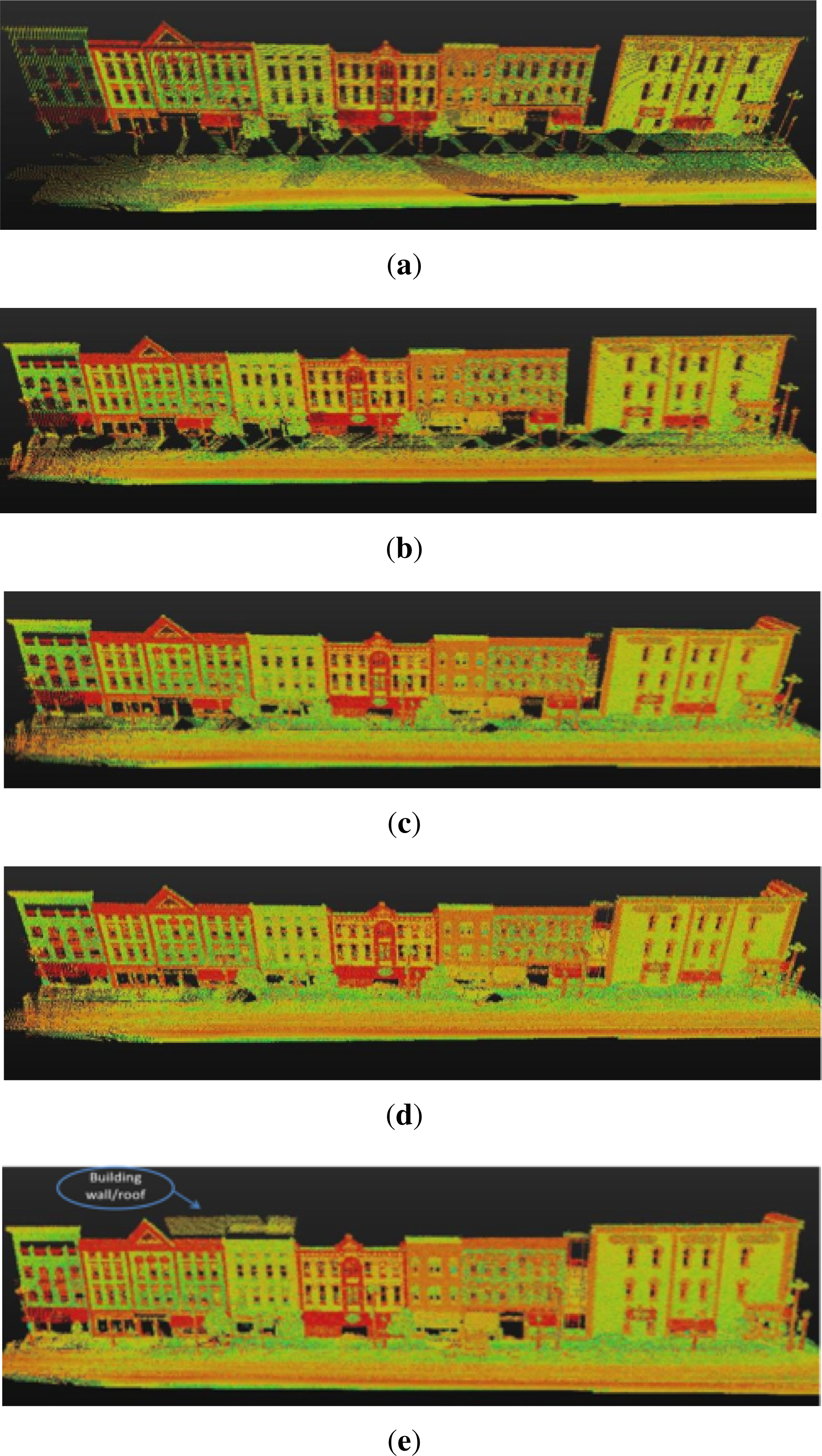
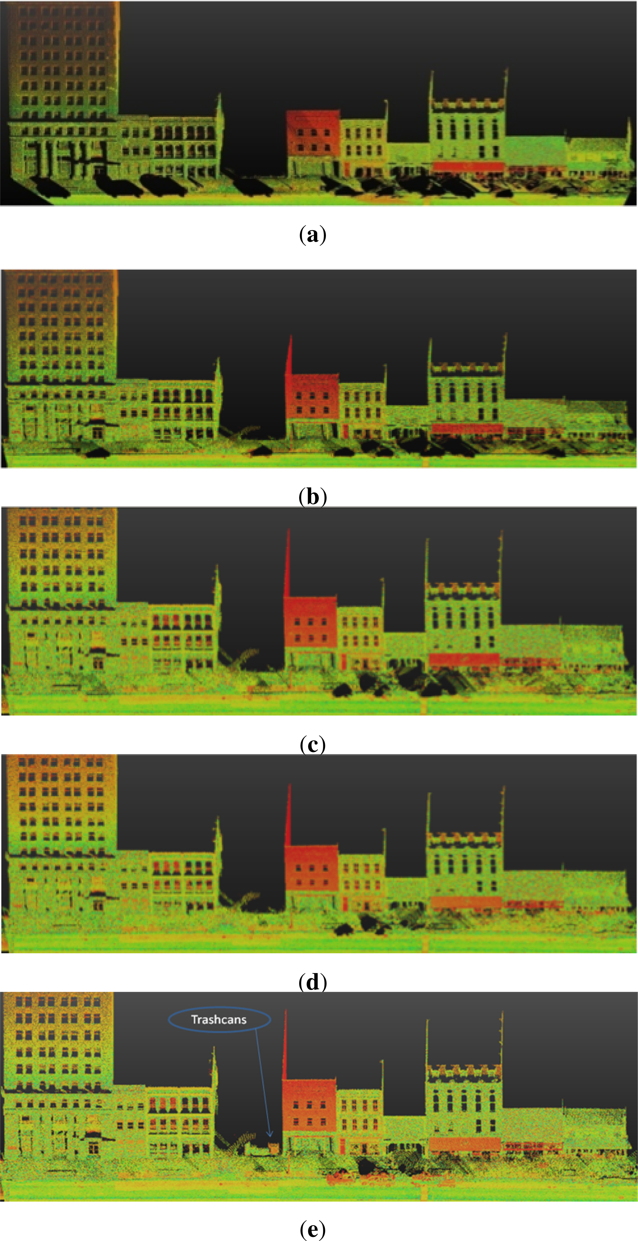
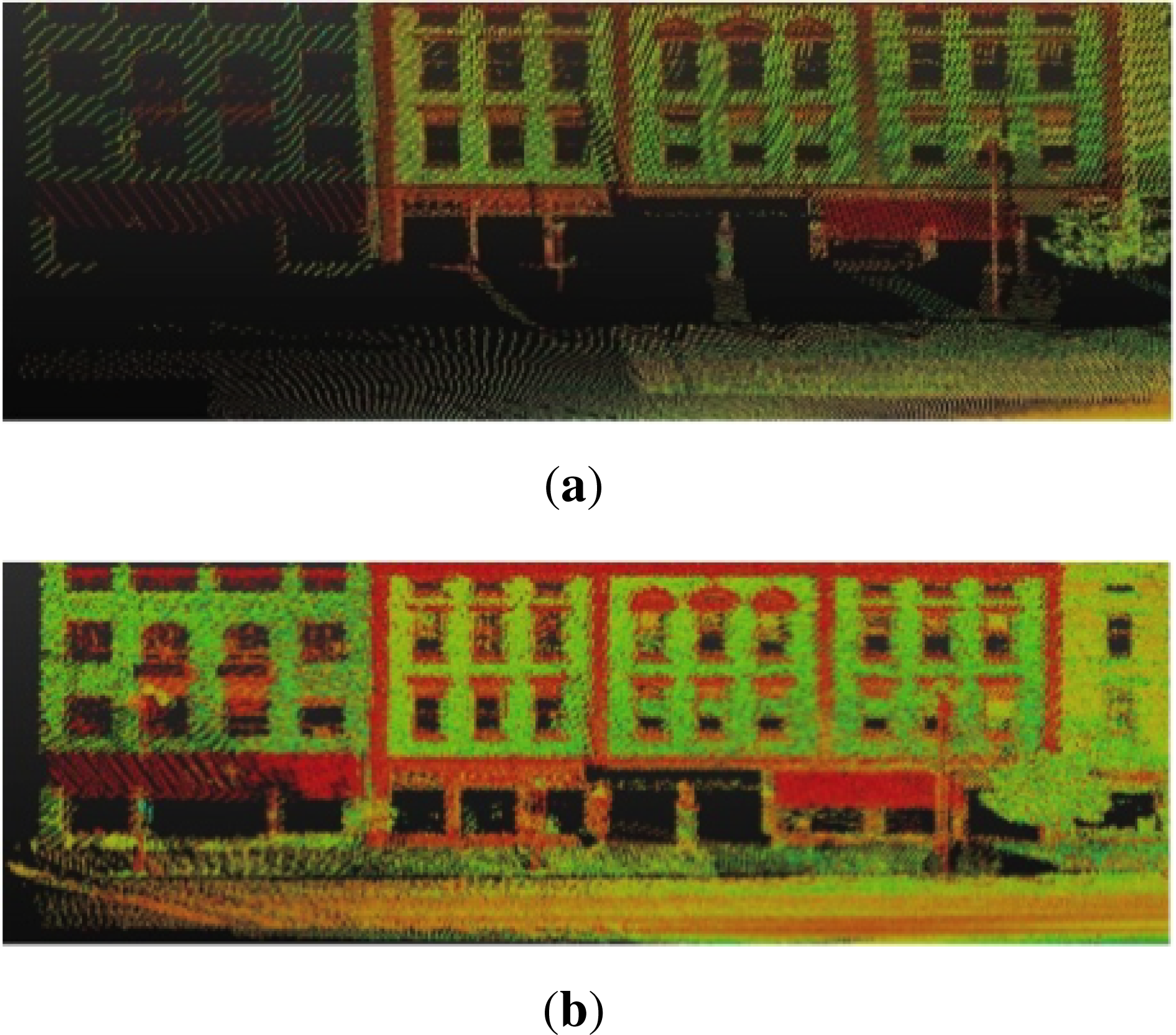
5. 3D Cartography and Removal of Imperfections Exploiting Multiple Passages

The perforated 3D point clouds obtained in subsequent passages of any particular place (on different days and/or at different times) are combined together to fill in the occluded regions and complete the 3D urban cartography. The perforated point cloud is first mapped onto a 3D evidence grid, and the corresponding 3D cell scores are calculated. A similarity map is generated in subsequent passages. Based on this similarity map and the associated uncertainty, different changes occurring in the urban environment are analyzed and appropriate actions are taken to cater for these changes. The details are provided below.

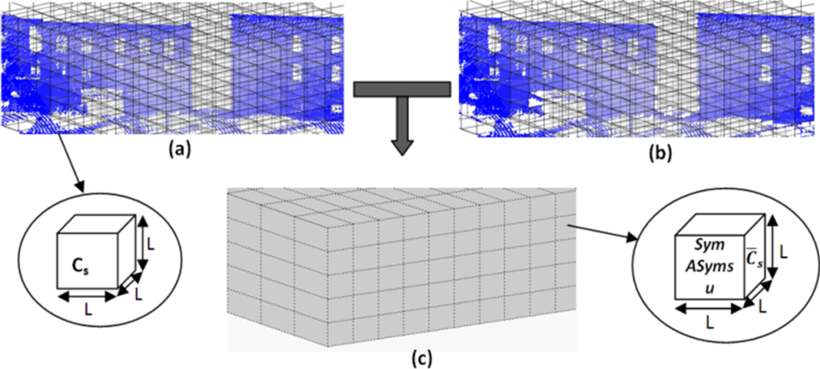
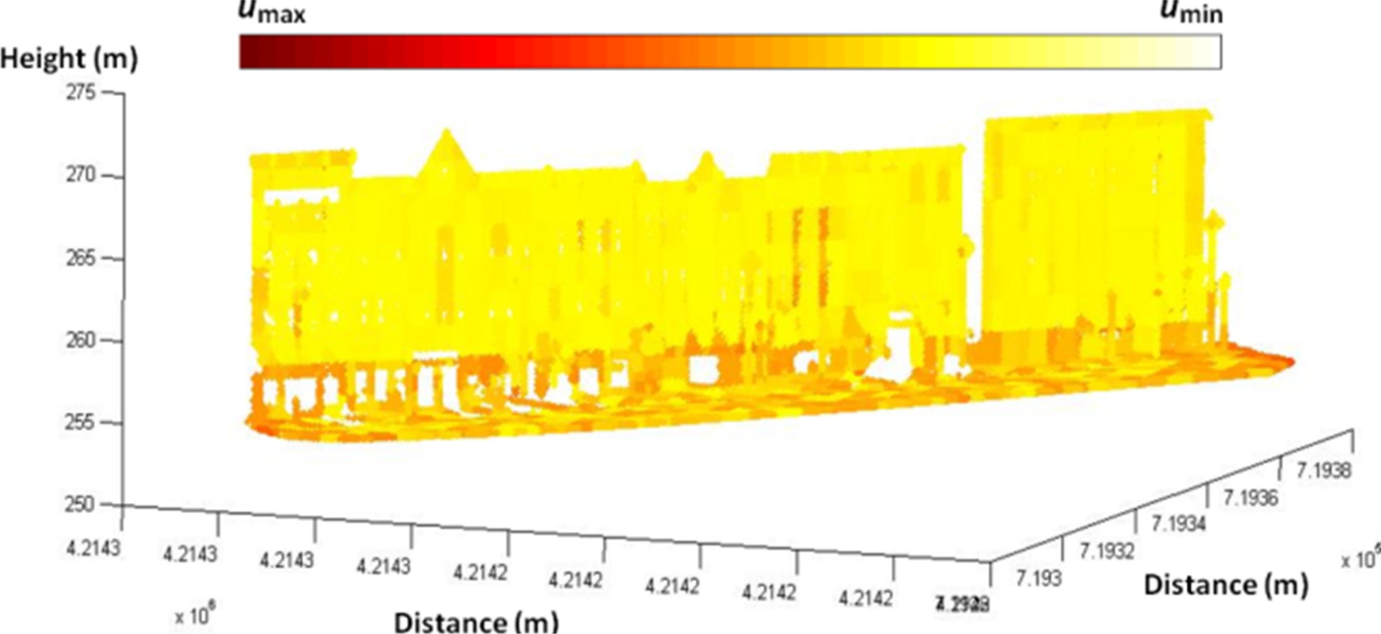
5.1. 3D Evidence Grid Formulation

As the 3D point cloud is directly geo-referenced, the use of an occupancy grid for comparison in subsequent passages as compared to the elaborate graph theory is more logical and practical. The perforated 3D point cloud obtained in each passage is mapped onto a 3D evidence grid, as shown in Figure 6. Each 3D cell or voxel of this grid occupies a volume, L3, and is assigned a cell score, CS, based on certain attributes of the constituting 3D points using Equation (4). These attributes include the ratio of occupied volume VOcc, surface normal along x-, y- and z-axes, NX,Y,Z, mean laser reflectance intensity and mean RGB color values, i.e., RI, Rc (c ∈ {R̄, Ḡ, B̄}), respectively, and the number of the current passage, np. The normalized values of these attributes are used to compute the cell score:
C S j = w O c c V O c c j + w N N X , Y , Z j + w R I R I j + w R c R c j + w n p n p w O c c + w N + w R I + w R c + w n p
where j is the number of cells. wOcc = 1 and wN = 0.5 are occupation weight and normal weight, while wRI = 0.25 and wRc = 0.125 are intensity and color weight, respectively. wnp = 0.0625 is the passage number weight. The values of these weights are chosen to bias the score more towards occupancy (magnitude and orientation) and less towards representation (intensity and color), as the former is more invariant in the urban environment and also keeps our approach closer to the classical occupancy grid method [32]. These 3D evidence grids are constructed in each passage for both the previous (P(np − 1)) and latest perforated 3D point cloud acquired and are used to formulate and update the similarity map along with the associated uncertainty. They are then deleted at the end of the process in each passage (Algorithm 1). This makes this approach most suitable for analyzing large mapping areas.

5.2. Similarity Map Construction

The 3D evidence grid in successive passages is compared to obtain a similarity map in each passage. Instead of finding the overall graph/grid similarity, we are more interested in measuring the similarity of each cell, as this indicates exactly which part of the 3D cartography has changed. Currently, many distances have been developed to compare two objects (in this case, cell) according to the type of attributes, such as χ2 or Mahalanobis. However, when working with real values, the most widely used (and simplest) metric is the Minkowski measure, dp:
d p ( x , y ) = [ i = 1 k W i | x i y i | p ] 1 p with p > 0
In this measure, xi and yi are the values of the ith attribute describing the individuals, x and y. Wi is the numerical weight correlated with this attribute. k is the total number of attributes. In order to transform Minkowski distance Equation (5) into a similarity measure, sp, a value, Di, is introduced, which corresponds to the difference between the upper and the lower bounds of the range of the ith attribute:
s p ( x , y ) = [ i = 1 k W i D i | x i y i | D i p ] 1 p with p > 0
This similarity function may provide a measure indicating the amount of changes occurring in a 3D grid cell in subsequent passages, but it remains silent on the type of change taking place. Now, this information could be useful when deciding how to handle these changes in the 3D cartography. Thus, in order to get more insight into the type of changes, we incorporate the notion of distance between individuals or objects studied in the cognitive sciences. For this purpose, we use the method proposed by Tversky [33] to evaluate the degree of similarity, Sx,y, between two individuals, x and y, respectively, described by a set of attributes, A and B, by combining the four terms, AB, AB, AB and BA, into the formula:
S x , y = f ( A B ) f ( A B ) + α f ( A B ) + β f ( B A )
As we want to compare a pair of individuals (in this case, cells in successive passages) described by a set of numerical attributes, we combine the definitions proposed by Tversky and Minkowski. In these measures, we use Tversky’s model to compare the two sets of attributes describing the individuals; the function, f, of this model is the Minkowski’s formula, as rewritten in Equation (6). The parameter, p, of this formula equals one, since in Tversky’s model, the function, f, corresponds to a linear combination of the features. Now, depending upon the way the parameters, α and β, are instantiated, different kinds of cognitive models of similarity can be expressed. By instantiating α = β = 0, we obtain the symmetric similarity measure, Sym, while by instantiating α = 0 and β = −1, we obtain the asymmetric similarity measure, ASym. Now, we use these values to fill up similarity map, SMap, as shown in Figure 6; the values of ASym allow us to evaluate the degree of inclusion between the first cell (reference) into the second cell (target). Hence, with the attributes (along with their corresponding weights) assigned to these cells (discussed in Section 5.1), the value of ASym can be used to assume the type of changes occurring in the 3D grid cell, as summarized in Table 2, where x and y are the same 3D grid cell in different passages. These values of Sym and ASyms help in ascertaining the most suitable function required for that particular 3D grid cell. Condition 1 is automatically handled by the default sequential update function, whereas for Condition 2 and 3, the automatic reset function is called into action.
The similarity map, SMap, is updated in each passage, and only the different cells (with Sym <Similaritythreshold) along with their associated uncertainty values are kept in the map, whereas the remaining cells considered as identical cells (with a high level of similarity) are deleted from the map. Hence, this not only reduces the size of the map progressively in subsequent passages, but also avoids possible storage memory issues for large point clouds in the case of large mapping areas. See Section 6.2 (Figure 7) for more details.

5.3. Associated Uncertainty

Let the cell scores of a particular cell, j, in n number of passages, C S 1 j , C S 2 j , , C S n j, be an iidsequence of random variables; then the nth sample variance s n j 2 is given as:
s n j 2 = k = 1 n ( C S k j C ¯ S n j ) 2 n 1
then, by adding and subtracting C ¯ S n 1 j:
s n j 2 = 1 n 1 [ k = 1 n ( C S k j C ¯ S n 1 j + C ¯ S n 1 j C ¯ S n j ) 2 ]
expanding and solving this to get:
s n j 2 = 1 n 1 [ ( n 2 ) s n 1 j 2 + ( n 1 ) ( C ¯ S n 1 j C ¯ S n j ) 2 + 2 k = 1 n 1 [ ( C S k j C ¯ S n 1 j ) ( C ¯ S n 1 j C ¯ S n j ) ] + ( C S n j C ¯ S n j ) 2 ]
Using the standard mean, ( k = 1 n 1 C S k j = ( n 1 ) C ¯ S n 1 j ), the sum-term simplifies to zero:
s n j 2 = [ ( n 2 ) s n 1 j 2 + ( n 1 ) ( C ¯ S j , n 1 C ¯ S n j ) 2 + ( C S n j C ¯ S n j ) 2 ] n 1
Further simplification yields:
s n j 2 = [ ( ( n 2 ) ( n 1 ) ) s n 1 j 2 + ( C S n j C ¯ S n 1 j ) 2 n ]
The uncertainty associated with each cell in the map, uj, is, hence, estimated and updated in each passage (n > 1) using the following relations:
u n j = [ ( ( n 2 ) ( n 1 ) ) ( u n 1 j ) 2 + ( C S n j C ¯ S n 1 j ) 2 n ] 1 2
where C ¯ S n j is the moving or running average given as:
C ¯ S n j = ( C S n j + ( n 1 ) C ¯ S n 1 j n )
There is no need to initialize Equations (8) and (9), as for n = 2, the first term in Equation (8) equals zero and in Equation (9), C ¯ S 1 j = C S 1 j. This uncertainty measure, updated using Equations (8) and (9), for each cell, in each passage, sheds light on the reliability of the state of the mapped cells as high uncertainty value means that the contents of the 3D cell are changing quite frequently; that could suggest high traffic circulation and other movements in the urban area. On the other hand, low uncertainty means that the contents of the 3D cell are fairly stable, indicating an established change (for example, permanent modifications in buildings or any other part of the cartography). This measure can also be added as a criterion for selecting the different specialized functions for the changing 3D cells; see Section 5.4.2 for more details. The uncertainty distribution of neighborhood-1 can be seen in Figure 8. The figure clearly shows a high level of uncertainty in the bottom part of the environment (close to the ground), due to different temporarily static and mobile objects present in the scene.

5.4. Specialized Functions

There are three specialized functions that are introduced in the method to make it more robust to different changes occurring in the urban environment and to remove different imperfections in the resulting cartography. These functions are described below.

5.4.1. Sequential Update Function

This is the default function (see Algorithm 1). It has two main purposes. Firstly, it offers a fine registration of the various 3D point clouds in subsequent passages. Secondly, it not only enriches the 3D point cloud by carefully adding 3D points in subsequent passages and, hence, completing the occluded regions in the process, but also automatically caters to the first type of change (Table 2) occurring in the urban environment.
Each subsequent 3D point cloud is registered with the former point cloud by using the ICP (Iterative Closest Point) method [34]. This method is most suitable for this task, as the 3D point clouds are already geo-referenced, hence lying in close proximity. It is observed that the major part of the 3D urban point clouds is composed of building points, which are also found to be most consistent. Thus, instead of applying the ICP method to complete 3D point clouds, only the building points are taken into account (see Algorithm 2). First, the profile/envelope of the buildings is extracted, and then, the ICP method is applied, matching these boundaries to obtain the transformation matrix. The outlines/envelopes of the buildings are extracted using a sweep scan method. As the bottom part of the building outline close to the ground is often occluded and, hence, inconsistent, due to the presence of different objects in the scene (see Figure 8), only the boundary of the top half of the building outline is subjected to ICP, as shown in Figure 9.
Algorithm 2. Extraction of outlines of buildings
Require: 3D points of building objects
 1: for minimum x and y values of 3D points to maximum x and y values of 3D points do
 2:  Scan building points in the xy plane
 3:  Find the maximum and minimum value in the z-axis
 4: end for
 5: for minimum z values of 3D points to maximum z values of 3D points do
 6:  Scan building points in the z-axis
 7:  Find maximum and minimum value in the xy plane
 8: end for
 9: return envelope/profile of building objects
Once the transformation matrix (rotation matrix Rm and translation matrix Tm) is found, the whole 3D point cloud, P(np), is transformed into P′(np) and, then, registered with the former P(np − 1) using Equation (10).
P ( n p ) = R m ( P ( n p ) ) + T m
In order to avoid redundant points, a union of 3D points belonging to the two registered images is performed. Each 3D point of the first point cloud is matched with that of the second, if Equation (11) is satisfied:
p O a p O b e tol 3
where pOa and pOb (3 × 1 vectors) are point positions in two point clouds along the x-, y- and z-axes. etol (3 × 1 vector) is equal to the inverse of the maximum number of 3D points per cubic meter that is desired in the 3D cartographic point cloud/image. The matched 3D points are considered as one point, i.e., the earlier point is retained, whereas the latter point is ignored. This ensures that only the missing points are added completing the perforated 3D point cloud/image.
Now, this specialized function also ensures that even if there is some new construction or addition of certain 3D points in the scene in subsequent passages, they are automatically added, hence catering for the first type of change (Table 2).

5.4.2. Automatic Reset Function

The main purpose of this function is to detect and analyze different changes occurring in the urban environment, over a number of passages, before incorporating them in the resulting 3D cartography. The function analyzes the similarity map, SMap, and compares the Sym, ASyms and the uncertainty measures, u, of the 3D cells after every nreset number of passages. Those 3D cells, C n j, which satisfy Conditions 2 and 3 (Table 2) along with a low value of uncertainty measure, u, Equation (12) are reset with those in the recently acquired image/point cloud (perforated), i.e., their contents are replaced by the contents of the same 3D cells in the recently acquired point cloud/image. This ensures that any changes that occur in the urban environment are automatically incorporated in the resulting 3D cartography in a very smooth manner without affecting the remaining part of the 3D cartography.
Reset ( C n j ) if m ( A S y m ( C m 1 j , C m j ) A S y m ( C m j , C m 1 j ) ) ( u n j < u threshold )
where m = {(nnreset) ⋯n}, with n > nreset. The proposed reset method was verified by synthetically modifying and demolishing different parts of the urban environment, including parts of buildings, roads and poles, in the datasets (for details, you can see Figure 10).
Now, Equation (12) ensures that a detected change is incorporated in the resulting cartography, only if we are certain about it. If the change is well-established, the uncertainty value of changing cells will progressively decrease, and when it falls below the uthreshold, these changes are incorporated in the 3D cartography via the reset function (as shown in Figure 11(a)). On the contrary, detected change with increasing or high uncertainty indicates the occurrence of rapid continuing changes, which could be either due to ongoing construction/reconstruction or rapid traffic movement in the scene (as shown in Figure 11(b)). In such situations, the detected changes are not incorporated at once, but in fact, we wait for the u to progressively decrease below uthreshold as the number of passages, np, increases. This ensures the reliability and accuracy of our method.

5.4.3. Object Update Function

This function caters to different misclassifications and other unclassified objects. With every new passage, once the urban cartography is completed, the objects classified in each passage as temporarily static are also analyzed using Equation (1)(3). If the same objects belonging to this class are found at the same place in repeated passages, they are then upgraded as permanently static objects and are considered part of the 3D cartography (Algorithm 1). They are then added to the 3D cartography. Otherwise, non-repetitive objects are deleted from the update register, R(np). This number of allowable repetitions, nupdate, can be fixed, based upon the frequency of repetition, time of repetition, etc. This not only allows gradual update of the 3D cartography, but also accommodates the unclassified objects in the scene; for example, certain parts of building walls in neighborhood-1 (Figure 12(e)) and a few roadside trashcans in neighborhood-2 (Figure 13(e)), which were unclassified, were added to the cartography, after repetition in the successive passages, during the update phase.

5.5. Automatic Checks and Balances

If certain 3D points or objects are wrongly added in the 3D cartography, due to either misclassification or certain repetitions in the object update function, these are then detected in subsequent passages as changes and, after analysis, are progressively removed by the automatic reset function. Hence, this ensures that the resulting 3D cartography contains only the exact, actual and permanent features.

6. Results, Evaluation and Discussion

In order to validate our method, the dynamic data set of the 3D Urban Data Challenge 2011 was used. This data set contains four sets of the same dynamic scenes of downtown Lexington, Kentucky, USA, obtained on different days and at different times. The data set consists of 3D points coupled with corresponding laser reflectance intensity values. As the corresponding RGB values are not readily available, Equation (2) was not used. This did not have much impact on the results, as laser reflectance values are found to be more consistent than RGB values in an urban environment, which is more illumination invariant [31]. The results for two different neighborhoods are discussed in this paper. In Figures 12 and 14, the detailed results for neighborhood-1, neighborhood-2 and neighborhood-1(modified) are presented, respectively. The figures clearly show how different imperfections are progressively removed using the specialized functions, while the different changes occurring in the urban scene are updated after successful detection and analysis. Figure 15 shows the successful completion of occluded features along with the imperfection removal of a particular street corner using this method.

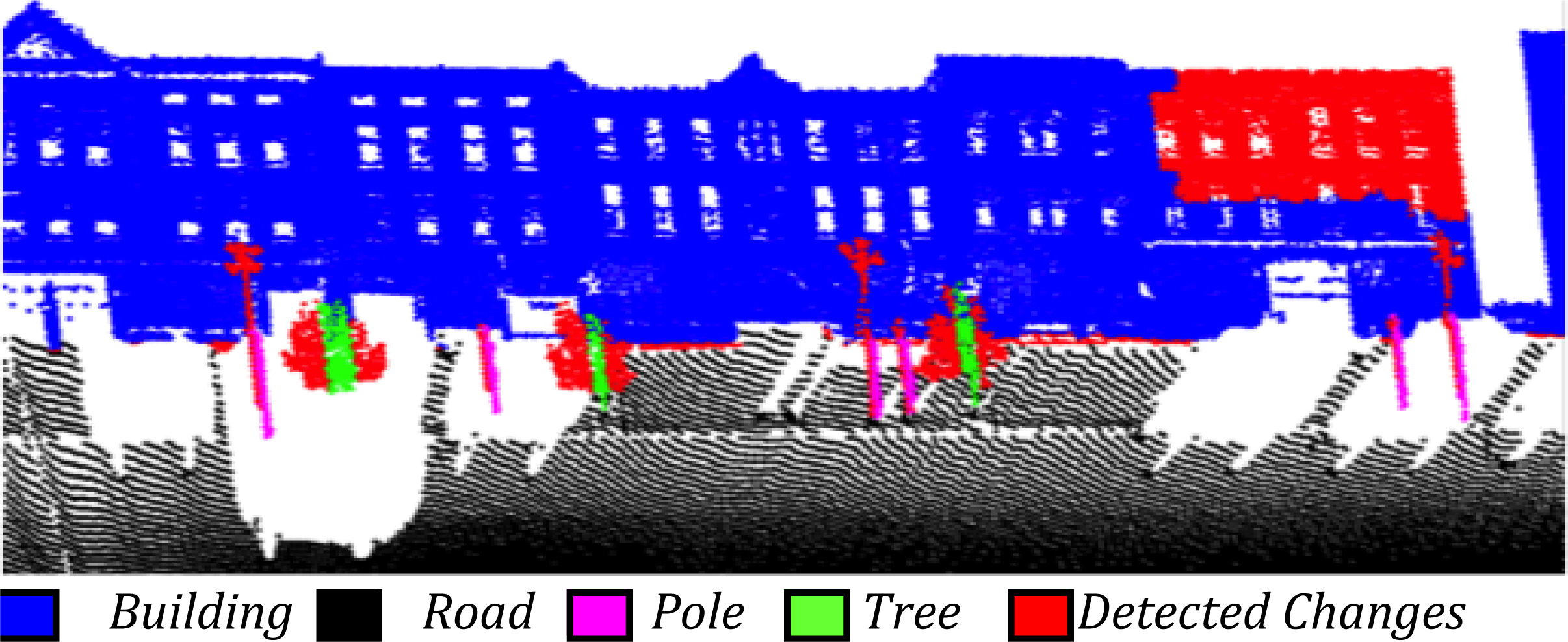
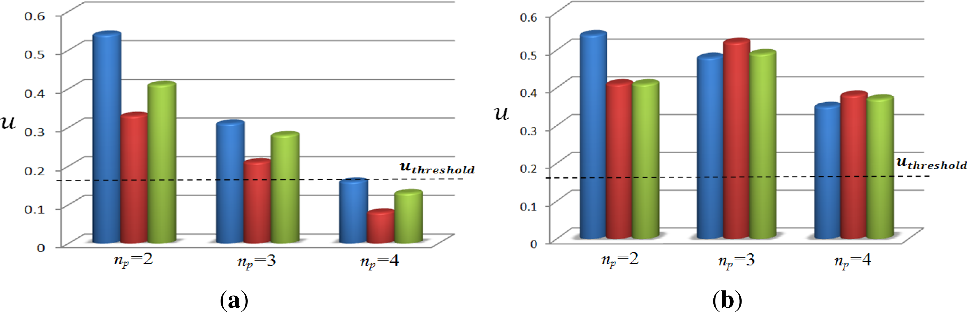
6.1. Change Detection and Reset Function

Now, in order to evaluate the reset function, we assessed the ability of the proposed method to successfully detect changes occurring in the urban environment before they can be updated in the cartography. We first constructed an ROC (Receiver Operating Characteristic) curve. The value of Similaritythreshold (used as a discriminatory threshold) was varied from zero to one, and corresponding true positive rates (TPR) and false positive rates (FPR) were calculated for neighborhood-1 (modified). The variation of this ROC curve with respect to uthreshold (varying from zero to 0.5) is presented by a 3D ROC curve (surface, in this case) in Figure 16. From the figure, it could be observed that the best/optimal results (A in the figure) can be obtained from Similaritythreshold = 66% and uthreshold = 0.15. This analysis was conducted at the 3D cell level. Figures 10 and 14(f) show some of these detected changes in the urban scene. These values of Similaritythreshold and uthreshold along with L = 2 m, etol = (0.000125 0.000125 0.000125)T (in m3) and nreset = 3 (the maximum number of passages possible in our case is four) were then used to evaluate the performance of our method for all three neighborhoods.
Change detection for the automatic reset function was evaluated using different standard evaluation metrics, as described in [35] (see Table 3). Although all these metrics are commonly used to evaluate such algorithms, MCC (Matthews Correlation Coefficient) is regarded as the most balanced measure, as it is insensitive to different class sizes (as is the case with our application, the number of changed cells (changes) is generally quite inferior as compared to unchanged cells in the urban environment). The MCC, like the other measures, is calculated based on the count of the true positives (i.e., correct detection of changed 3D cells), false positives, true negatives and false negatives. A coefficient of +1 represents a perfect prediction, zero is no better than random prediction and −1 indicates total disagreement. The detailed results, including the overall accuracy, ACC, and MCC greater than 85% and +0.6, respectively, clearly demonstrate the efficacy of the proposed method.

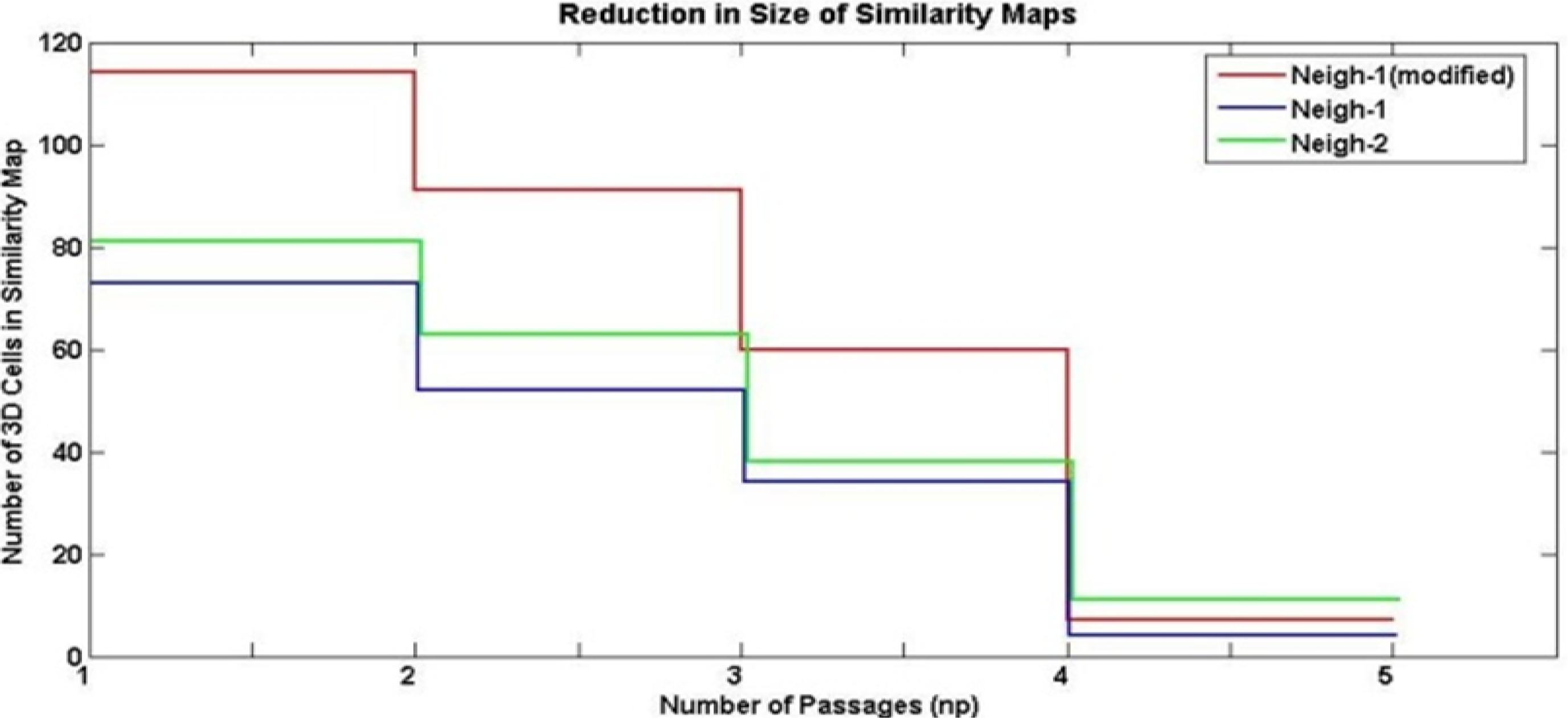
6.2. Evolution of Similarity Map Size

Figure 7 shows the progressive reduction of the size of the similarity map in subsequent passages. This is due to the fact that in subsequent passages, as occluded regions are completed, the number of low similarities caused by the missing occluded features decreases, and also, the different changes occurring in the cartography are catered to by means of the automatic reset function. In the case of neighborhood-1 (modified), Figure 7, the large size of SMap is due to large parts of the building, poles, trees, etc., being demolished in neighborhood-1 (see Figure 10), whereas a sharp decrease in size occurs at np = 4, due to the automatic reset function (nreset = 3). We see that some non-repeating cells or those with high associated uncertainty remain even after the automatic reset. This number of cells in the SMap should ideally reduce to zero as the number of np increases.

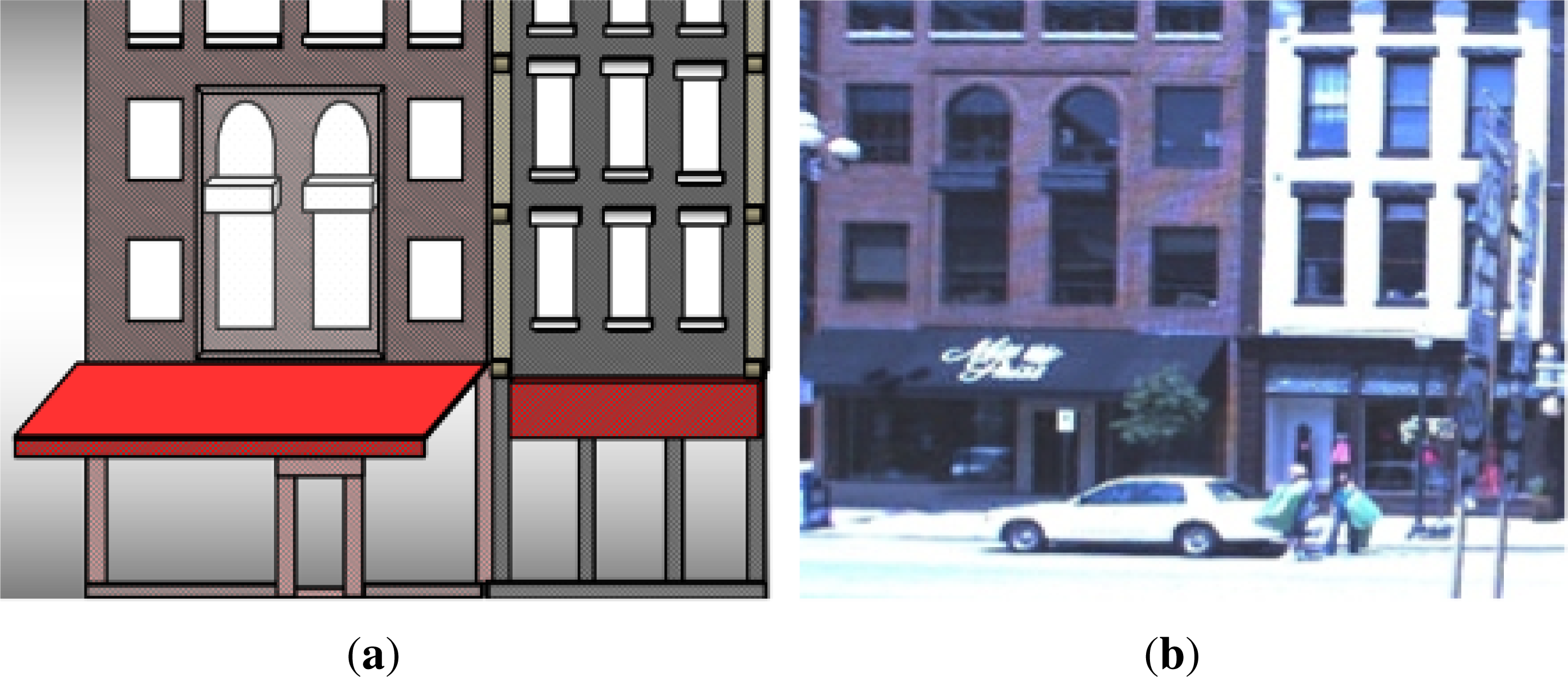
6.3. Handling Misclassifications and Improvement in Classification Results

To assess the removal of imperfections due to misclassification, the improvement in classification results by the proposed method as compared to single passage classification (standard practice) was evaluated using standard F -measure as described in [35,36]:
F β = ( 1 + β 2 ) p . r ( β 2 . p + r )
where p and r are the precision and recall, respectively, and β is the weight constant. Table 4 shows that the proposed method improves the classification results (permanently static objects are analyzed here, as they constitute the permanent cartography, and, hence, are of most interest to us). The value of β = 1 was used to obtain a balanced F1 score. The classified objects were considered as a percentage of their constituting points in the 3D scene. This improvement is due to different misclassifications being progressively corrected, hence reducing the imperfections caused by them in the resulting 3D cartography.

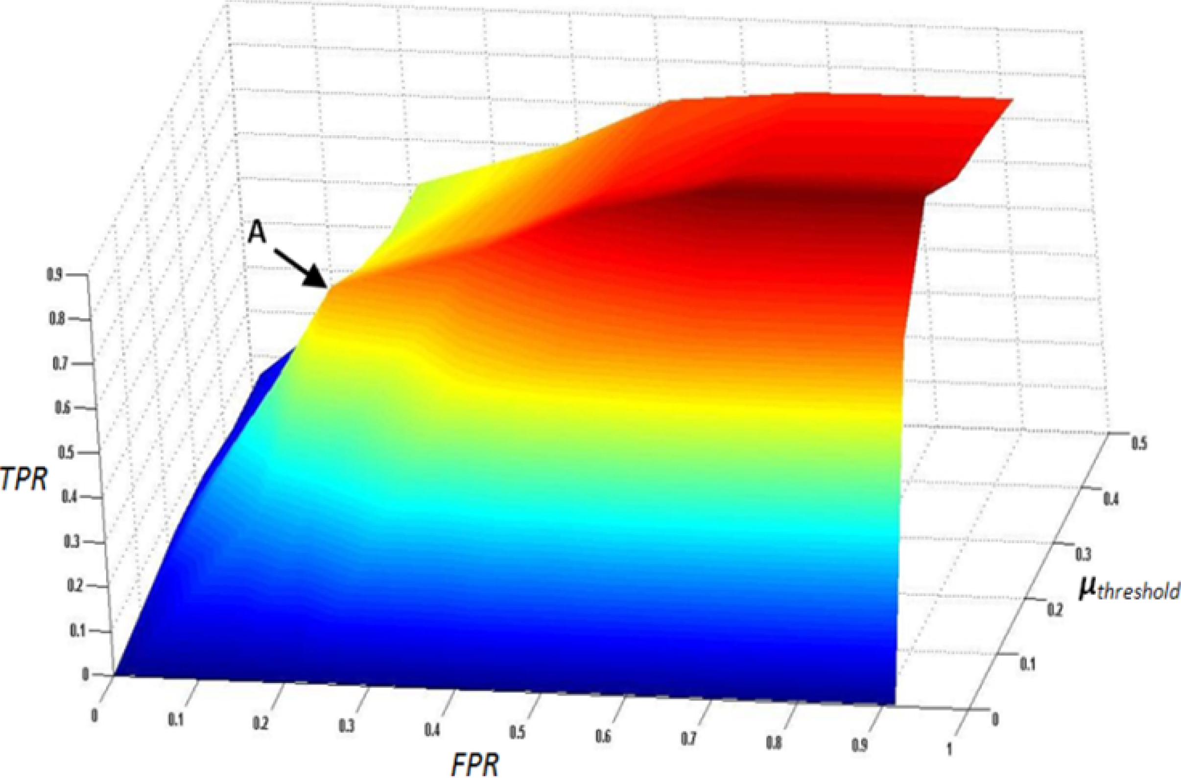
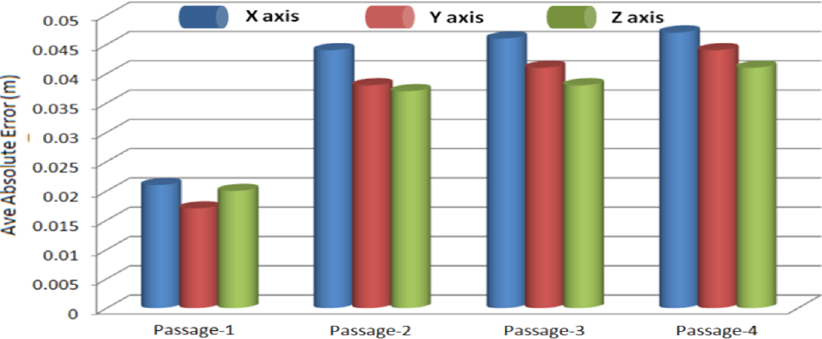
6.4. Accuracy Evaluation

In order to evaluate the accuracy of the completed permanent features/regions and, hence, the effectiveness of the imperfection removal, we selected a corner building in neighborhood-1. As no ground truth was readily available, we generated the ground truth by creating a simplified 3D model of the building using standard CAD software, as shown in Figure 17. The 3D points from the initial acquisition were used for this purpose, while the missing features were completed by horizontal and vertical interpolations, exploiting the symmetry of the building design; these features were confirmed/matched with the images of the building, from different viewing angles, acquired by the digital spherical camera mounted on the vehicle (see Figure 17). A number of features, including the occluded ones, were selected for comparison. The dimensions of these selected features extracted in the 3D image obtained at each passage, using our method, were then compared with their corresponding dimensions in the ground truth. The average absolute errors in x-, y- and z-axes (height) of the available dimensions obtained in each passage are presented in Figure 18. These error values include both registration and sensor measurement errors. Low average absolute error values obtained for passage-1 are due to the fact that part of these 3D points was used for ground truth generation. These generally low and fairly constant error values make this method suitable for most applications.

7. Conclusions

In this work, we have presented a new method for automatic 3D urban cartography that progressively removes different imperfections caused by occlusions, misclassifications of objects in the scene and ineffective incorporation of changes occurring in the environment over time, by taking advantage of incremental updating using specialized functions. Different changes occurring in the urban landscape are automatically detected and analyzed using cognitive functions of similarity, and the resulting 3D cartography is modified accordingly. The proposed method ensures that the resulting 3D point cloud of the cartography is quite reliable, and it contains only the exact and actual permanent features, free from imperfections.
The results evaluated on a real data set using different evaluation metrics demonstrate the technical prowess of the method. The thorough analysis exhibits accurate change detection (including values of overall accuracy ACCand a Matthew’s Correlation Coefficient (MCC) greater than 85% and +0.6, respectively), improved classification results (with a standard F1 score > 0.98) and high accuracy of the completed permanent features/regions of the urban cartography. The results also show that the method is well scalable and that it can both be easily integrated and ideally suited for removing various imperfections for different commercial or non-commercial applications pertaining to urban landscape modeling and cartography requiring frequent database updating.

Acknowledgments

This work is supported by the Agence Nationale de la Recherche (ANR-the French national research agency) (ANR CONTINT iSpace & Time–ANR-10-CONT-23) and by “le Conseil Général de l’Allier”. This work has also been funded by the French government research program, Investissements d’avenir, through the RobotEx Equipment of Excellence (ANR-10- EQPX-44) and the IMobS3 Laboratory of Excellence (ANR-10-LABX-16-01) by the European Union through the program, Regional competitiveness and employment 2007–2013 (ERDF—Auvergne region), by the Auvergne region and by the French Institute for Advanced Mechanics.

Conflict of Interest

The authors declare no conflict of interest.

References

  1. Wang, C.; Thorpe, C.; Thrun, S.; Hebert, M.; Durrant-Whyte, H. Simultaneous localization, mapping and moving object tracking. Int. J. Robot. Res 2007, 26, 889–916. [Google Scholar]
  2. Vögtle, T.; Steinle, E. Detection and recognition of changes in building geometry derived from multitemporal laserscanning data. Int. Arch. Photogramm. Remote Sens. Spat. Inf. Sci 2004, 35, 428–433. [Google Scholar]
  3. Champion, N.; Everaerts, J. Detection of unregistered buildings for updating 2D databases. EuroSDR Off. Publ 2009, 56, 7–54. [Google Scholar]
  4. Criminisi, A.; Pérez, P.; Toyama, K. Region filling and object removal by exemplar-based inpainting. IEEE Trans. Image Process 2004, 13, 1200–1212. [Google Scholar]
  5. Wang, L.; Jin, H.; Yang, R.; Gong, M. Stereoscopic inpainting: Joint color and depth completion from stereo images. Proceedings of IEEE Conference on Computer Vision and Pattern Recognition (CVPR), Anchorage, AK, USA, 23–28 June 2008; pp. 1–8.
  6. Engels, C.; Tingdahl, D.; Vercruysse, M.; Tuytelaars, T.; Sahli, H.; van Gool, L. Automatic occlusion removal from façades for 3D urban reconstruction. Proceedings of Advanced Concepts for Intelligent Vision Systems, Ghent, Belgium, 22–25 August 2011; pp. 681–692.
  7. Barnes, C.; Shechtman, E.; Finkelstein, A.; Goldman, D. PatchMatch: A randomized correspondence algorithm for structural image editing. ACM Trans. Graph 2009, 28, 24:1–24:11. [Google Scholar]
  8. Konushin, V.; Vezhnevets, V. Automatic Building Texture Completion. Proceedings of Graphicon’2007, Moscow, Russia, 23–27 June 2007; pp. 174–177.
  9. Rasmussen, C.; Korah, T.; Ulrich, W. Randomized View Planning and Occlusion Removal for Mosaicing Building Façades. Proceedings of IEEE/RSJ International Conference on Intelligent Robots and Systems (IROS 2005), Edmonton, AB, Canada, 2–6 August 2005; pp. 4137–4142.
  10. Bénitez, S.; Denis, E.; Baillard, C. Automatic production of occlusion-free rectified façade textures using vehicle-based imagery. Int. Arch. Photogramm. Remote Sens. Spat. Inf. Sci 2010, 38, 275–280. [Google Scholar]
  11. Xiao, J.; Fang, T.; Zhao, P.; Lhuillier, M.; Quan, L. Image-based street-side city modeling. ACM Trans. Graph 2009, 28, 114:1–114:12. [Google Scholar]
  12. Ortin, D.; Remondino, F. Occlusion-free image generation for realistic texture mapping. Int. Arch. Photogramm. Remote Sens. Spat. Inf. Sci. 2005, 36, Part 5/W17. 7. [Google Scholar]
  13. Böhm, J. A Multi-image fusion for occlusion-free façade texturing. Int. Arch. Photogramm. Remote Sens. Spat. Inf. Sci 2004, 35, 857–873. [Google Scholar]
  14. Craciun, D.; Paparoditis, N.; Schmitt, F. Multi-view scans alignment for 3D spherical mosaicing in large-scale unstructured environments. Comput. Vision Image Underst 2010, 114, 1248–1263. [Google Scholar]
  15. Becker, S.; Haala, N. Combined feature extraction for façade reconstruction. Int. Arch. Photogramm. Remote Sens. Spat. Inf. Sci 2007, 36, 44–49. [Google Scholar]
  16. Frueh, C.; Sammon, R.; Zakhor, A. Automated Texture Mapping of 3D City Models with Oblique Aerial Imagery. Proceedings of IEEE 2nd International Symposium on 3D Data Processing, Visualization and Transmission (3DPVT), Thessaloniki, Greece, 6–9 September 2004; pp. 396–403.
  17. Li, Y.; Zheng, Q.; Sharf, A.; Cohen-Or, D.; Chen, B.; Mitra, N.J. 2D-3D Fusion for Layer Decomposition of Urban Façades. Proceedings of IEEE International Conference on Computer Vision (ICCV), Barcelona, Spain, 6–13 November 2011.
  18. Matikainen, L.; Hyyppä, J.; Kaartinen, H. Automatic detection of changes from laser scanner and aerial imagedata for updating building maps. Int. Arch. Photogramm. Remote Sens. Spat. Inf. Sci 2004, 5, 3413–3416. [Google Scholar]
  19. Vu, T.T.; Matsuoka, M.; Yamazaki, F. LIDAR-Based Change Detection of Buildings in Dense Urban Areas. Proceedings of 2004 IEEE International Geoscience and Remote Sensing Symposium, Anchorage, AK, USA, 20–24 September 2004; 5, pp. 3413–3416.
  20. Bouziani, M.; Goïta, K.; He, D.C. Automatic change detection of buildings in urban environment from very high spatial resolution images using existing geodatabase and prior knowledge. ISPRS J. Photogramm 2010, 65, 143–153. [Google Scholar]
  21. Matikainen, L.; Hyyppä, J.; Ahokas, E.; Markelin, L.; Kaartinen, H. Automatic detection of buildings and changes in buildings for updating of maps. Remote Sens 2010, 2, 1217–1248. [Google Scholar]
  22. Schäfer, T.; Weber, T.; Kyrinovič, P.; Zámečniková, M. Deformation Measurement Using Terrestrial Laser Scanning at the Hydropower Station of Gabčíkovo. Proceedings of INGEO 2004 and FIG Regional Central and Eastern European Conference on Engineering Surveying, Bratislava, Slovakia, 11–13 November 2004.
  23. Lindenbergh, R.; Pfeifer, N. A Statistical Deformation Analysis of Two Epochs of Terrestrial Laser Data of a Lock. Proceedings of ISPRS 7th Conference on Optical 3D Measurement Techniques, Vienna, Austria, 3–5 October 2005; 2, pp. 61–70.
  24. Van Gosliga, R.; Lindenbergh, R.; Pfeifer, N. Deformation analysis of a bored tunnel by means of terrestrial laser scanning. Int. Arch. Photogramm. Remote Sens. Spat. Inf. Sci 2006, 36, 167–172. [Google Scholar]
  25. Hsiao, K.; Liu, J.; Yu, M.; Tseng, Y. Change detection of landslide terrains using ground-based LiDAR data. Int. Arch. Photogramm. Remote Sens. Spat. Inf. Sci 2004, 35, 617–621. [Google Scholar]
  26. Girardeau-Montaut, D.; Roux, M.; Marc, R.; Thibault, G. Change detection on points cloud data acquired with a ground laser scanner. Int. Arch. Photogramm. Remote Sens. Spat. Inf. Sci 2005, 36, 30–35. [Google Scholar]
  27. Hyyppä, J.; Jaakkola, A.; Hyyppä, H.; Kaartinen, H.; Kukko, A.; Holopainen, M. others. Map Updating and Change Detection Using Vehicle-Based Laser Scanning. Proceedings of 2009 IEEE Joint Urban Remote Sensing Event, Shanghai, China, 20–22 May 2009; pp. 1–6.
  28. Zeibak, R.; Filin, S. Change detection via terrestrial laser scanning. Int. Arch. Photogramm. Remote Sens. Spat. Inf. Sci 2007, 36, 430–435. [Google Scholar]
  29. Kang, Z.; Lu, Z. The Change Detection of Building Models Using Epochs of Terrestrial Point Clouds. Proceedings of 2011 IEEE International Workshop on Multi-Platform/Multi-Sensor Remote Sensing and Mapping (M2RSM), Xiamen, China, 10–12 January 2011; pp. 1–6.
  30. McDonald, J.; Kaess, M.; Cadena, C.; Neira, J.; Leonard, J. Real-time 6-DOF multi-session visual SLAM over large-scale environments. Robot. Auto. Syst. 2012. [Google Scholar] [CrossRef]
  31. Aijazi, A.K.; Checchin, P.; Trassoudaine, L. Segmentation based classification of 3D urban point clouds: A super-voxel based approach with evaluation. Remote Sens 2013, 5, 1624–1650. [Google Scholar]
  32. Souza, A.A.; Gonçalves, L.M. 3D Robotic Mapping with Probabilistic Occupancy Grids. Int. J. Eng. Sci. Emerg. Technol 2012, 4, 15–25. [Google Scholar]
  33. Tversky, A. Features of similarity. Psychol. Rev 1977, 84, 327–352. [Google Scholar]
  34. Besl, P.; McKay, N. A method for registration of 3-D shapes. IEEE Trans. Pattern Anal. Mach. Intell 1992, 14, 239–256. [Google Scholar]
  35. Vihinen, M. How to evaluate performance of prediction methods? Measures and their interpretation in variation effect analysis. BMC Genomics 2012, 13, S2. [Google Scholar]
  36. Hripcsak, G.; Rothschild, A.S. Agreement, the F-measure, and reliability in information retrieval. J. Am. Med. Inform. Assoc 2005, 12, 296–298. [Google Scholar]
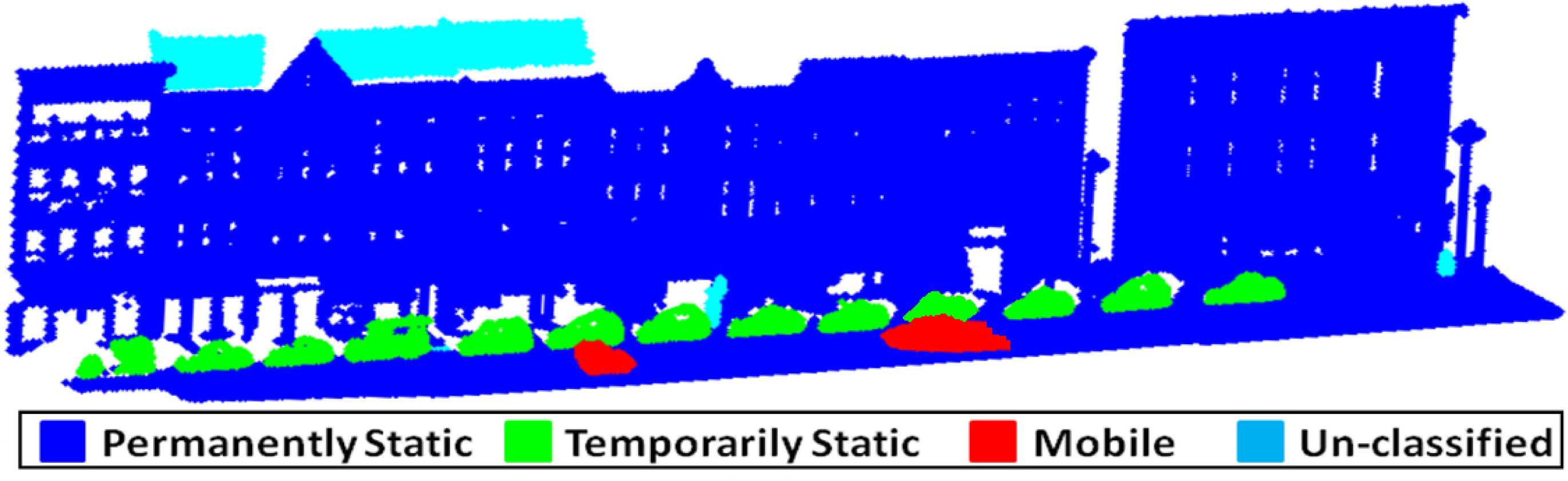
Figure 1. (a) The Vis Center’s LiDAR truck; (b) Optech LiDAR/GPS system along with IMU mounted on a rigid frame; (c) the different viewing angles of the mounted LiDAR systems.
Remotesensing 05 03701f1
Figure 2. (a) Voxel-based segmentation of a particular scene; (b) classified 3D points.
Remotesensing 05 03701f2
Figure 3. 3D points of moving vehicles in the urban scene. In red, the 3D points acquired from S − 01, and in white, the 3D points acquired from S − 02.
Remotesensing 05 03701f3
Figure 4. Classification of the objects present in the urban scene into three main classes.
Remotesensing 05 03701f4
Figure 5. The objects classified as temporarily static and mobile are extracted out from the scene, leaving behind a perforated point cloud for each passage.
Remotesensing 05 03701f5
Figure 6. Formulation of 3D evidence grids and similarity map. ((a) and (b)) show the 3D point clouds (P(np) and P(np − 1)) mapped onto an evidence grid of cell size, L3, respectively. In (c), the similarity map obtained from the two evidence grids.
Remotesensing 05 03701f6
Figure 7. The progressive reduction of the size of similarity map, SMap.
Remotesensing 05 03701f7
Figure 8. Uncertainty distribution map of the busy neighborhood-1 presented in the form of a color-coded heat map (with yellow being the lowest and red the highest level of uncertainty). The map clearly shows that the bottom part of the environment (close to the ground) is highly uncertain, whereas the top part is generally stable.
Remotesensing 05 03701f8
Figure 9. In red and blue, the building outline obtained from the first passage. In green and black, the outline obtained from the second passage. Only the top half of the two outlines in blue and black, respectively, is subjected to Iterative Closest Point (ICP).
Remotesensing 05 03701f9
Figure 10. The different changes detected in one of the urban scenes are presented in red. These changes were due to a demolished building wall, larger poles cut in half and trimming/cutting of bushes/trees in the scene.
Remotesensing 05 03701f10
Figure 11. The uncertainty, u, variation of a group of three adjacent cells in which change was detected. (a) represents the case of established changes, while (b) represents the case of rapid or continuing changes.
Remotesensing 05 03701f11
Figure 12. (a) Shows the initial point cloud related to urban cartography full of imperfections. In (b), (c) and (d), completion of occluded and missing features in the urban cartography, by incremental updating, using the default sequential update function as a change of type-1 is detected. (e) shows the point cloud after the object update function; certain parts of the roadside and building walls are added to the 3D cartography after repetition in subsequent passages. (a) 3D point cloud, P(np), after first passage; (b) 3D point cloud, P(np), after second passage; (c) 3D point cloud, P(np), after third passage; (d) 3D point cloud, P(np), after fourth passage; (e) 3D point cloud, P(np), after object update.
Remotesensing 05 03701f12
Figure 13. (a) shows the initial point cloud related to urban cartography full of imperfections. In (b), (c) and (d), completion of occluded and missing features in the urban cartography, by incremental updating, using the default sequential update function as a change of type-1 is detected. (e) shows the point cloud after the object update function; certain parts of the roadside and building walls along are added to the 3D cartography after repetition in subsequent passages. (a) 3D point cloud, P(np), after first passage; (b) 3D point cloud, P(np), after second passage; (c) 3D point cloud, P(np), after third passage; (d) 3D point cloud, P(np), after fourth passage; (e) 3D point cloud, P(np), after object update.
Remotesensing 05 03701f13
Figure 14. (a) shows the initial point cloud related to urban cartography full of imperfections. In (b), (c) and (d), completion of occluded and missing features in the urban cartography, by incremental updating, using the default sequential update function as a change of type-1 is detected. In (e), the automatic reset function came into action after changes of type 2&3 were detected, to update the modifications in the 3D cartography. (f) shows the point cloud after the object update function; certain parts of the roadside and building walls are added to the 3D cartography after repetition in subsequent passages. On (f) are also marked the changes successfully detected and updated after four passages. These include: 1—building wall/roof added, due to initial misclassification; 2—part of building demolished; 4, 5 and 6—trimmed or cut trees/bushes; 3, 7 and 8—longer poles cut in half. (a) 3D point cloud, P(np), after first passage; (b) 3D point cloud, P(np), after second passage; (c) 3D point cloud, P(np), after third passage; (d) 3D point cloud, P(np), after fourth passage; (e) 3D point cloud, P(np), after automatic reset; (f) 3D point cloud, P(np), after object update.
Remotesensing 05 03701f14aRemotesensing 05 03701f14b
Figure 15. Different missing features and imperfections belonging to shop windows, walls, pole and road in (a) are successfully completed and removed in (b), respectively, using this method for neighborhood-1. (a) 3D point cloud, P(np), after first passage; (b) 3D point cloud, P(np), after fourth passage.
Remotesensing 05 03701f15
Figure 16. True positive rate (TPR) is plotted against false positive rate (FPR) to obtain a 3D Receiver Operating Characteristic (ROC) curve for neighborhood-1 (modified). Point A on the surface represents the optimal/best results.
Remotesensing 05 03701f16
Figure 17. (a) shows the generated 3D model of the buildings according to dimensions; In (b), one of the camera images of the building is presented.
Remotesensing 05 03701f17
Figure 18. Average absolute errors in x, y and z (height) directions.
Remotesensing 05 03701f18
Table 1. Object classification chart.
Object TypePermanently StaticTemporarily StaticMobile
Roadx
Buildingx
Treex
Polex
Carxx
Pedestrianxx
Unclassifiedxx
Table 2. Type of changes.
#ConditionPossible Assumption
1ASymx,y< ASymy,xAddition of structure (could be new construction)
2ASymx,y> ASymy,xRemoval of structure (could be demolition)
3ASymx,y = ASymy,xModification of structure (depending on the value of Sym)
Table 3. Change detection evaluation.
Neighborhood 1 (Modified)Neighborhood 1Neighborhood 2
ACCAccuracy0.8640.8910.903
PPVPositive Predictive Value0.8420.8500.900
NPVNegative Predictive Value0.8640.9020.901
FDRFalse Discovery Rate0.1580.1500.100
F1F1 measure0.6950.6500.782
MCCMatthews Correlation Coefficient+0.624+0.692+0.729
Table 4. Classification results for permanently static objects (F1-Score).
Passage 1Passage 2Passage 3Passage 4Proposed Method
Neighbor-10.9430.9770.9580.9590.981
Neighbor-20.9790.9750.9810.9840.992

