1. Introduction
Soil erosion is considered to be a major environmental problem since it seriously threatens natural resources, agriculture and the environment [
1]. It is one of the main processes that reduce soil productivity by removing fertile topsoil layers [
2]. Moreover, soil erosion often causes negative downstream effects, such as the sedimentation of soil material in reservoirs and lakes or damage to infrastructural facilities [
3]. Disastrous environmental consequences caused by soil erosion can be in the form of overflow from rivers or reservoirs subsequent to soil erosion, pollution of natural waters, or adverse effects on soil secondary salinisation. Overall, serious soil erosion has been and is degrading soil and water resources. It leads to the degeneration of climatic and ecological environments, and hinders the development of society and economy.
China is country with some of the worst soil erosion in the world. Soil erosion has always been the number one eco-environmental problems in China. According to the investigation result of “comprehensive scientific investigation on soil erosion and ecological security in China” took place from 2005–2007, the area of soil erosion of China was 3.57 × 10
6 km
2, which accounts for almost 14.2% of the world’s soil erosion area [
4]. Water erosion was the main type of soil erosion, which accounted for 45% of the total area of soil erosion. The water erosion area was divided into five classes with light, moderate, severe, more severe and extremely severe, accounting for 51.4%, 32.7%, 10.7%, 3.7% and 1.5% of the total water erosion area, respectively [
5]. The annual soil erosion amount in China in recent years has reached 4.5 billion tons. The annual average soil erosion modulus of major rivers has reached 3,400 t/km
2/yr, which is far higher than the soil loss tolerance and also higher than other serious soil erosion countries [
4].
The Danjiangkou reservoir area is the main water source and the submerged area of the Middle Route South-to-North Water Transfer Project of China. It has larger population density, prominent conflicts between human and land, and a fragile ecological environment. The forest structure is incoordinate, with mainly middle aged and young forest, which leads to poor vegetation protection ability. Combined with high mountains and steep slopes, exposed rock mass loose, destruction of vegetation, cultivation on steep slopes and other irrational land use, runoff erosion is much more likely to happen. Research show that water erosion is the main type of soil erosion, which accounted for 99% in the total area of soil erosion. The rill and sheet erosion is the leading form of water erosion encountered in the study area [
6]. Soil erosion in the Danjiangkou reservoir area can reduce soil productivity and lead to damaged drainage networks and infrastructural facilities, soil material sedimentation in reservoirs, flooding, and water pollution. Therefore, the spatial distribution and dynamic changes of the erosion risk in the Danjiangkou reservoir area should be assessed to control soil erosion and protect the ecological environment.
Existing soil erosion assessment methods include qualitative methods that identify erosion risk and quantitative methods that measure precise erosion rates. The qualitative methods include visual interpretation [
7,
8], index integration [
9,
10], and image classification [
11,
12]. The quantitative methods include erosion model [
13–
19], digital elevation model [
20,
21], nuclear tracing [
22–
25], and neural network method [
26]. Among them, the most widely used experienced statistical model are Universal Soil Loss Equation (USLE) [
27], which estimates long-term average annual soil loss and Revised Universal Soil Loss Equation (RUSLE), which is a revised method of USLE methodology incorporating additional data [
28]. The most representative physical model is Water Erosion Prediction Project (WEPP) model which is a process-based, distributed parameter, continuous simulation, erosion prediction model [
29].
However, validating the results of erosion rates is difficult because accurate measurements are generally expensive and time consuming and standard equipment is hardly available [
30]. The use of remote sensing images has proved successful in monitoring soil erosion changes in time and space [
31–
33]. It has proved to be a straightforward and inexpensive tool in erosion risk assessment [
34–
39]. In qualitative methods, the qualitative factors integration firstly classifies some major factors based on specific standard, and the classified factors are then integrated according to certain formula to create an erosion risk map [
40]. This method is used widely because it is rarely influenced by personal subjective knowledge, and when combined with geographic information systems (GIS) can efficiently and quickly monitor erosion risk [
41].
Based on remote sensing and GIS, the qualitative analysis of the dynamic changes of the spatial distribution and intensity of the soil erosion can provide an important basis for soil erosion assessment, control, and prediction. This analysis is significance in the sustainable utilisation of land resources and water environment safety. It also provides derivations of the scientific basis for ecological construction and sustainable development of social economy.
The objective of this study is to assess the water erosion (rill and sheet erosion) risk and dynamic change trend of spatial distribution in erosion status and intensity between 2004 and 2010 in the Danjiangkou reservoir area using a multicriteria evaluation method, which synthesizes the vegetation fraction cover, slope gradient, and land use. The study results will assist government agencies in determining erosion control areas, starting regulation projects, and making soil conservation measures.
2. Materials and Methods
2.1. Study Area
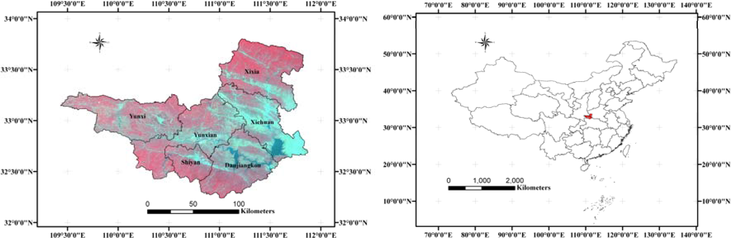
The study area is located in the middle and upper reaches of the Hanjiang River basin, between the northwest of Hubei and the southwest of Henan Province (
Figure 1). The total area is about 17,924 km
2 (109°29′–111°53′E, 31°30′–33°48′N), and it includes Danjiangkou, Yunxian, Yunxi, Shiyan, Xixia, and Xichuan. The study area is located in the Qinling-Bashan climatic region, which is the climatic transitional region from North to South China. It has the characteristics of a north subtropical zone continental monsoon climate, with four different seasons, adequate rainfall and sunshine. The climate is affected by monsoon and terrain. The average annual temperature is about 14 °C–16 °C, and the average annual sunshine ranges from 1,500 h to 1,980 h. Inhomogeneous temporal distribution of rainfall can be observed in the study area. The annual precipitation in a rainy year is 1,500 mm and in a low flow year is 500 mm. The spatial distribution of precipitation is from the east to the west regressive. According to a 50-year recorded period of precipitation in the area (1959–2008), the annual mean precipitation is about 804 mm.
The study area crosses the two first-order tectonic units, Yangtze para-platform and the Qinling folded mountain system, with fault development, complex geological structures, and loose surface rock stratum. The major geomorphic types are hill, low mountain, middle mountain, and high mountain. The range of vertical distribution is from the elevation of 500 m–800 m. The minor geomorphic types are river valley flatland and intermontane basin.
The soil types include paddy soil, mountain brown soil, yellow brown soil, limestone soil, moisture soil and purple soil. Yellow brown soil and paddy soil are mainly observed in slope land and paddy field, respectively. Considering the soil from diverse soil parent materials and the poor erosion resistance capacity of the major soil, the superaddition of inhomogeneous spatial and temporal distributions of rainfall, and the rain storms caused by precipitation concentration, soil disintegration and translocation easily occur in the area under raindrop splash erosion [
6,
42]. The main vegetation types of the area include coniferous forest, broad-leaved forest, shrubland, and coniferous and broad-leaved mixed forest. The vegetation cover exhibits an uneven distribution, and the vegetation cover rate of low mountains and hills is lower than that of the middle and high mountain regions.
2.2. Datasets
One multi-spectral HJ-1B CCD2 image was acquired on 17 June 2010. Three Landsat TM5 images were acquired on 17 May 2004 (Path125/Row37 and Path125/Row38) and 25 June 2004 (Path126/row37). The images were geometric correction and atmospheric correction. HJ-1B is a new generation of small Chinese civilian Earth-observing optical RS satellites. The wide-coverage multispectral CCD camera has four bands of blue, green, red and shortwave infrared spectral wavelengths (B1:0.43–0.52 μm, B2:0.52–0.60 μm, B3:0.63–0.69 μm, B4:0.76–0.90 μm). The CCD camera has nadir pixel resolution of 30 m, width of view of 360 km and central-pixel matching accuracy of 0.3 pixels [
43]. Landsat TM has seven spectral bands, three in the visible range and four in the infrared range (B1: 0.45–0.52 μm, B2:0.53–0.61 μm, B3:0.63–0.69 μm, B4:0.78–0.90 μm, B5:1.55–1.75 μm, B6:10.4–12.5 μm, B7:2.09–2.35 μm). The band wavelengths were chosen for their value in discriminating vegetation type, water penetration, plant and soil moisture measurements, and identification of hydrothermal alteration in certain rock types. All of the bands have a 30 m pixel size except band 6.
A Digital Elevation Model (DEM) was used for the study to generate slope. The DEM of 30 m pixel size was provided by the Ministry of Economy, Trade and Industry of Japan and the National Aeronautics and Space Administration.
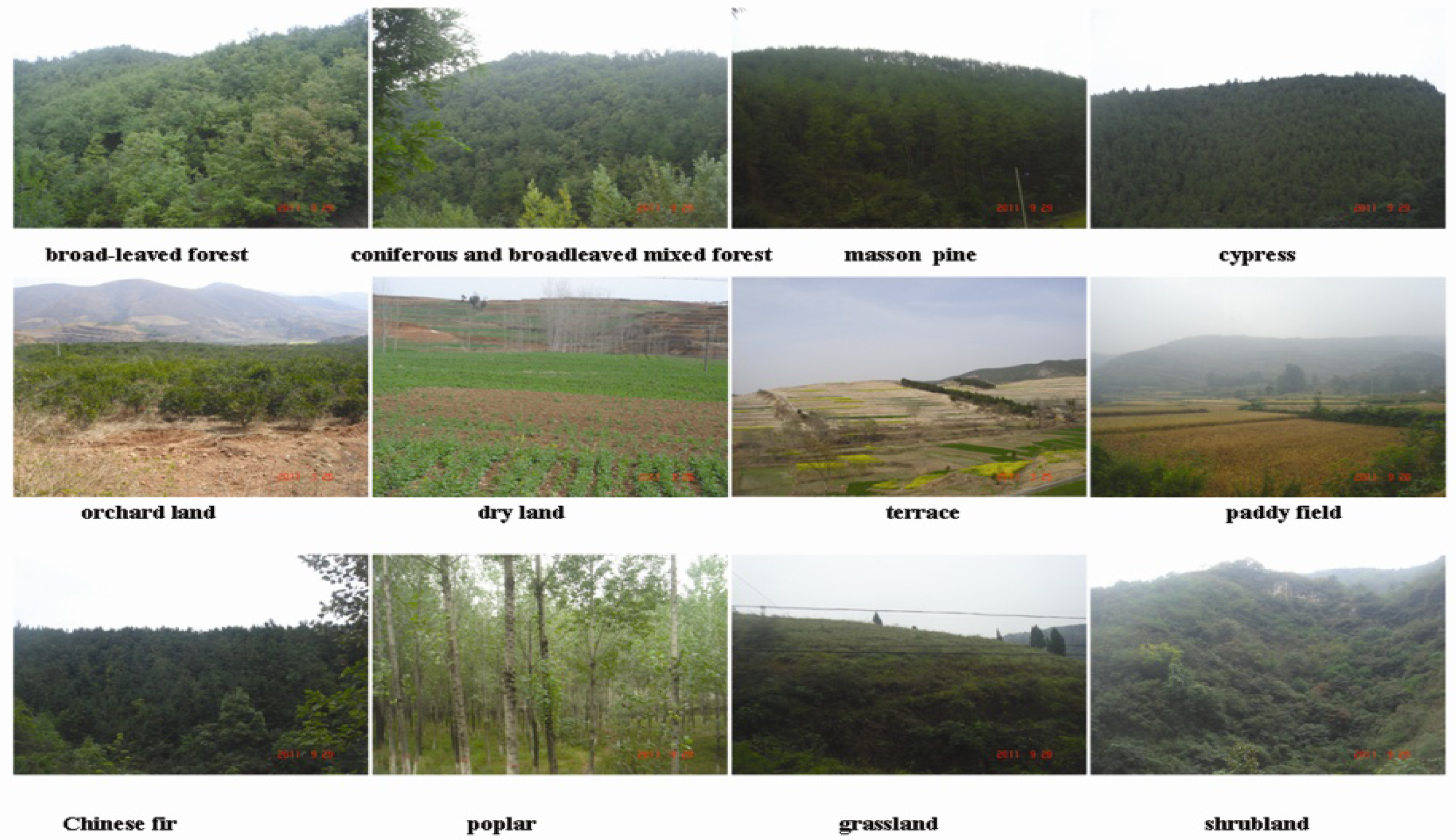
Field data were collected in March 2010 and in March and September 2011. A total of 238 random samples were selected in the study area. The land cover types of the samples include broad-leaved forest, coniferous forest (
i.e., masson pine, cypress, and Chinese fir), coniferous and broad-leaved mixed forest, cultivated land, orchard land, grassland, and scrubland (
Figure 2).
2.3. Methodology
2.3.1. Overview of the Methodology
The rate and magnitude of soil erosion are controlled by the following factors: terrain, vegetation fraction cover, rainfall intensity and runoff, soil erodibility, and land cover. The intensity, duration, and frequency of rainfall are the power factors of soil loss and are controlled by climate, whereas vegetation fraction cover and slope gradient, among others, are the factors indicating erosion resistance or risk. Therefore, the risk of soil erosion can be assessed based on the interactions between the slope, vegetation cover, and land-use type for rill and sheet erosion [
40].
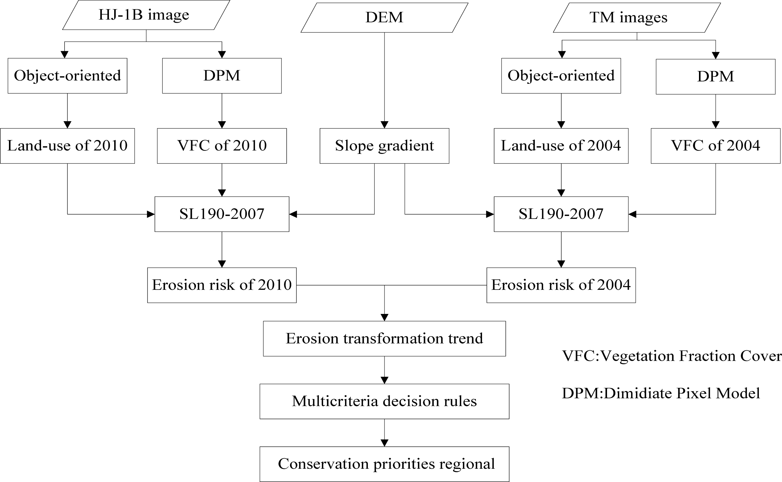
According to the national professional standards SL190-2007 for classification and gradation of erosion risk [
44], the flowchart illustrating of the overall methodology that used in this study is shown in
Figure 3. The methodology used to assess erosion risk requires three parameters as inputs: slope gradient, land-use, and vegetation fraction cover. The slope gradient is calculated using DEM. The land-use map and vegetation fraction cover are extracted from Landsat TM in 2004 and HJ-1B in 2010, respectively. In this study, the soil erosion risk was divided into six grades based on the aforementioned factors: slight, light, moderate, severe, more severe, and extremely severe (
Table 1). The ranges of average erosion modulus of each soil erosion risk are shown in
Table 2.
2.3.2. Slope Gradient Calculation
Topography is a crucial surface characteristic in soil erosion modelling [
45] and slope gradient has a significant influence on surface runoff and soil erosion [
45,
46]. In this study, slope gradient was computed based on the slope model in ARCGIS. The rate of change (delta) of the surface in the horizontal (
Slopewe) and vertical (
Slopesn) directions from the centre cell determines the slope gradient. The slope gradient algorithm can be interpreted as [
47]:
The values of the centre cell and its eight neighbours determine the horizontal and vertical deltas. The neighbours are identified as letters from “
e1” to “
e8”, with “
e” representing the cell for which the aspect is calculated. The rate of change in the horizontal and vertical directions for cell “
e” is calculated with the following algorithm:
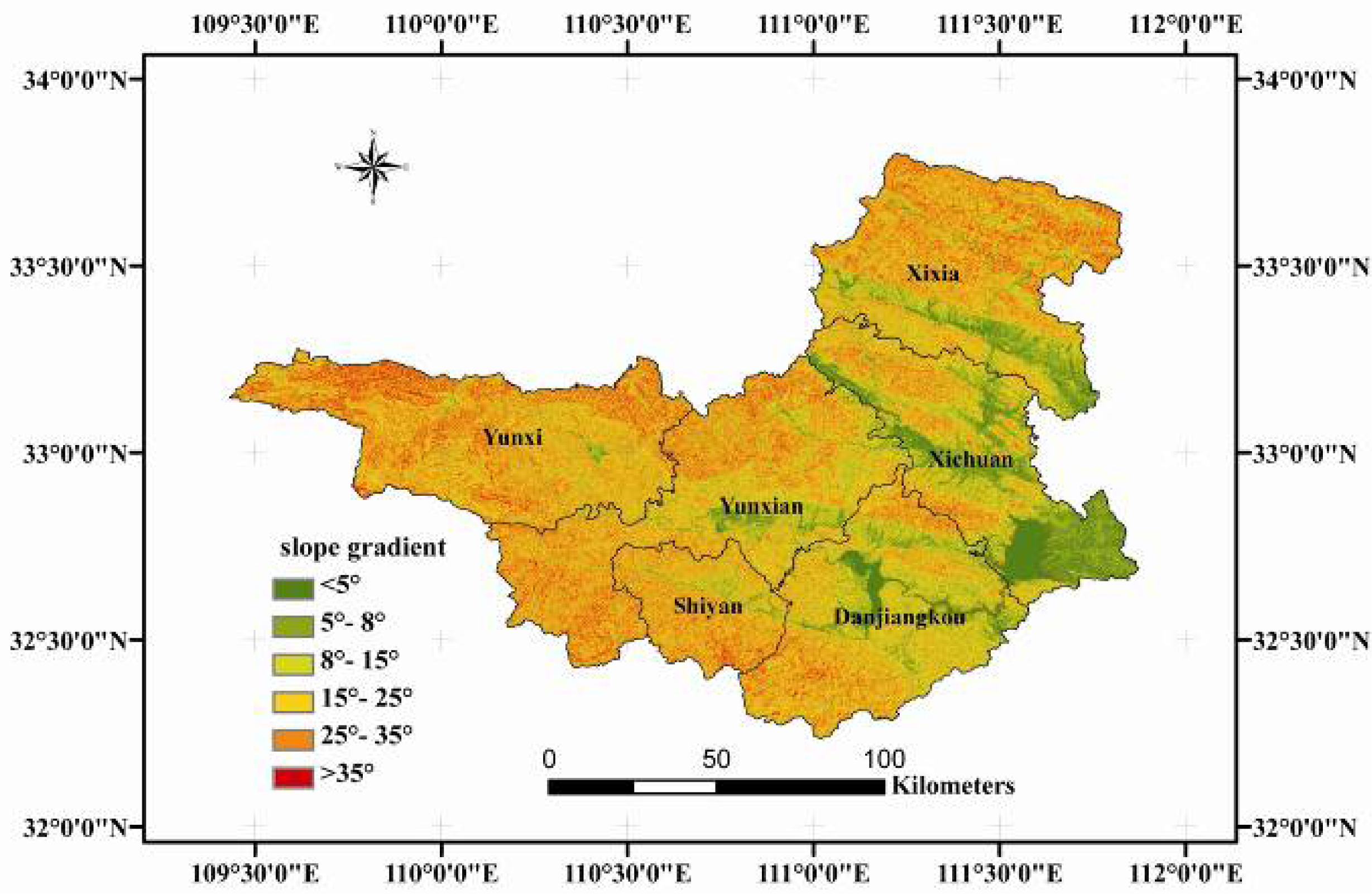
According to the national professional standards SL190-2007, the slope gradient in the study area was divided into six classes with limits of 5°, 8°, 15°, 25°, and 35° (
Figure 4).
2.3.3. Land-Use Mapping
It has been demonstrated that the object-oriented method could produce more accurate and robust classifications than pixel-based methods when using high-resolution imagery [
48–
51]. For instance, Myint
et al. [
49] demonstrate that the object-based classifier achieved a high overall accuracy in the city of Phoenix used QuickBird image data (90.40%), whereas the most commonly used decision rule, namely maximum likelihood classifier, produced a lower overall accuracy (67.60%). Roostaei
et al. [
50] show that the maximum likelihood classifier method has achieved an overall accuracy of 69% with kappa coefficient of 0.67, neural network classification 92% overall accuracy with a kappa coefficient of 0.90 and object-oriented with 94% overall accuracy and 0.92 coefficient kappa and the object oriented has superior performance in classifying vegetation and water areas.
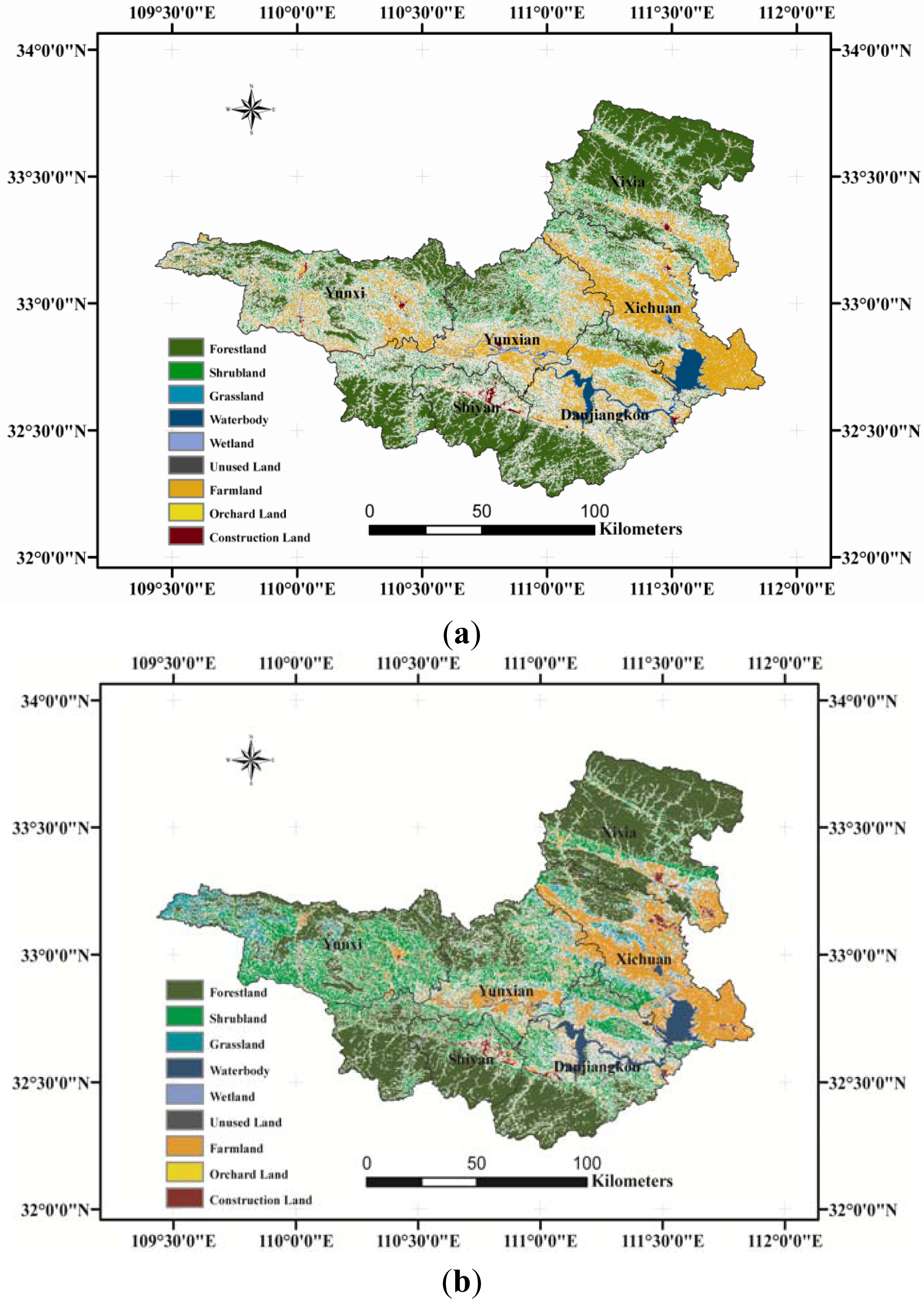
Assisted by field observation samples, the Landsat TM5 in 2004 and HJ-1B in 2010 were classified using eCognition, which is the original object-based image analysis software. The land-use results have nine classes: forestland, shrubland, grassland, cultivated land, orchard land, construction land, water body, wetland (according to the definitions and classifications of the US Fish and Wildlife Service), and unused land (
i.e., bare rock, beach land and bare ground). A human visual interpretation was used after the computer classification. The object which was misclassified by computer classification will be modified in ARCGIS. The land use maps of the study area in 2004 and 2010 are shown in
Figure 5. The overall accuracy of land use classification was more than 90% after human visual interaction interpretation and calibration based on field data. In erosion risk assessment, the land-use results were reclassified into four major land cover types: cultivated land, non-cultivated land (
i.e., forestland, shrubland, grassland, orchard land, wetland, and unused land), water body, and construction land. Erosion risks of cultivated land and non-cultivated land were assessed according to the national professional standard SL190-2007. The water body and construction land were considered non-soil erosion risk.
2.3.4. Estimation of Vegetation Fraction Cover
Vegetation fraction cover plays the most important role in soil erosion control [
2,
52]. The decrease in erosion rates with increasing vegetation cover is exponential [
53]. Plant and residue cover protects the soil from raindrop impact and splash, tends to slow down the movement of surface runoff, and enables excess surface water to infiltrate.
The value of radiant energy emitted from each pixel of the land surface can be divided into two parts: barren soil and vegetation. Therefore, the ratio of energy from vegetation to total energy can represent the vegetation cover of the pixel. Although many new vegetation indices have been established with the purpose of reducing the sensitivity to atmospheric conditions and substrate reflectivity, we selected Normalised Difference Vegetation Index (NDVI) because of its traditional use in deriving vegetation variables.Thus, the dimidiate pixel model was developed to quantify vegetation cover from the NDVI, which is derived from the near-infrared band (0.7 μm–1.1 μm) and the red band (0.4 μm–0.7 μm) of the remote sensing data.
where
NIR is the near-infrared band and
R is the red band of the image. Vegetation fraction cover is calculated by the formula.
where
VFC is the vegetation fraction cover,
NDVIsoil is the
NDVI value of the pure pixel of barren soil, and
NDVIveg is the
NDVI value of the pure pixel of vegetation.
It has been demonstrated that the dimidiate pixel model is an efficient algorithm for vegetation fraction cover estimation [
54–
59]. Several approaches have been proposed for retrieving the
NDVIveg and
NDVIsoil values from image. One of these approaches consists of choosing the minimal and maximal
NDVI values for the whole scene as
NDVIveg and
NDVIsoil. Although the assumption that
NDVIveg =
NDVImax could be appropriate, special care should be taken when assuming that
NDVIsoil =
NDVImin, as in most cases, the minimal
NDVI could be negative due to the presence of water bodies or other surfaces with negative
NDVI values. And due to the inevitable noise effect, it may produce too low or too high NDVI value. To avoid the wrong result, the minimal and maximal
NDVI values for the whole scene doesn’t directly as
NDVIveg and
NDVIsoil, but for the maximum and minimum
NDVI values in a given confidence level within the confidence interval. Confidence value is mainly decided by the image size and definition,
etc. Accordingly, in this study, the maximal
NDVI value is selected with 97% confidence value from the NDVI histogram, and the minimum
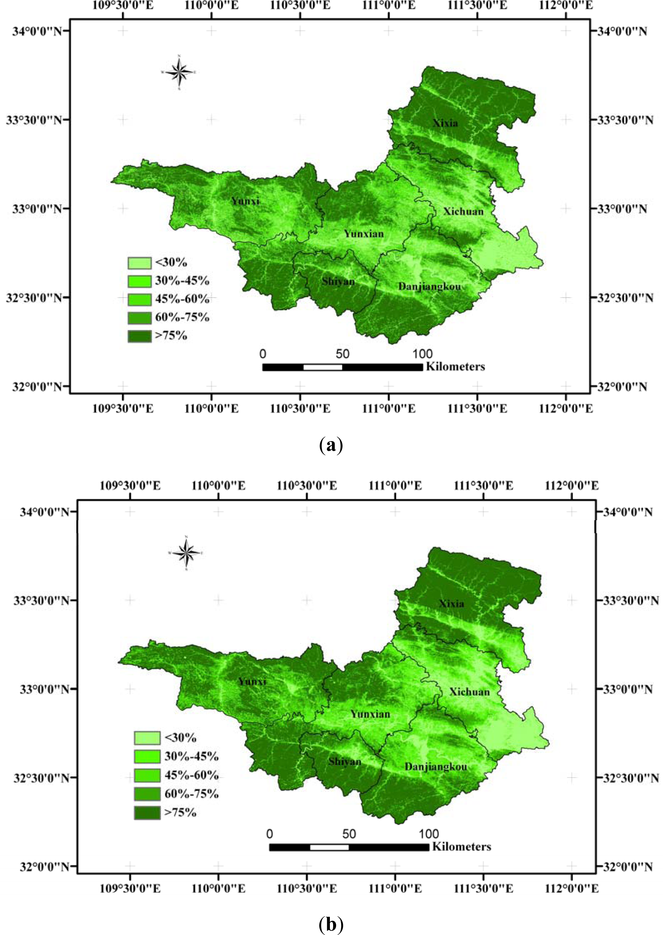
NDVI value is selected with 3% confidence value. Based on these analyses, this study estimated the vegetation fraction cover using the dimidiate pixel method. And according to the national professional standards SL190-2007, the vegetation fraction covers of the study area in 2004 and 2010 were divided into five classes with limits of 30%, 45%, 60%, and 75% (
Figure 6).
3. Results
3.1. Soil Erosion Risk Assessment
The slope gradient in the Danjiangkou reservoir area was divided into six classes with limits of 5°, 8°, 15°, 25°, and 35°, accounting for 8.66%, 8.57%, 20.89%, 30.29%, 21.28%, and 10.31% of the total study area, respectively. The vegetation fraction covers of the study area in 2004 and 2010 were divided into five classes with limits of 30%, 45%, 60%, and 75%, with each class of the year 2004 accounting for 19.82%, 11.75%, 12.46%, 12.95%, and 43.02% of the total area, respectively, and each class of the year 2010 accounting for 16.10%, 11.63%, 13.67%, 16.52%, and 42.08% of the total area, respectively.
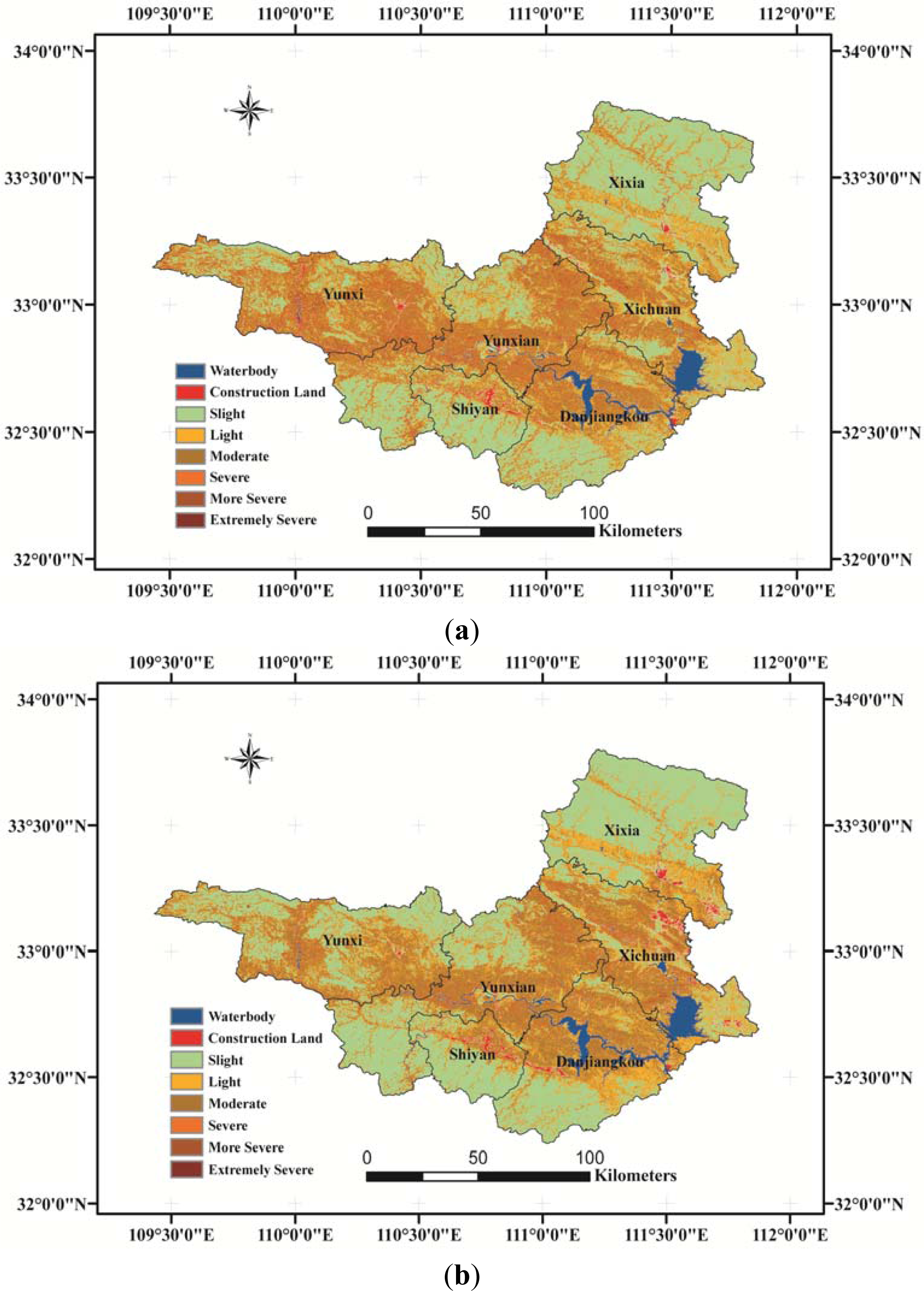
The erosion risk of the study area in 2004 (
Figure 7a) and 2010 (
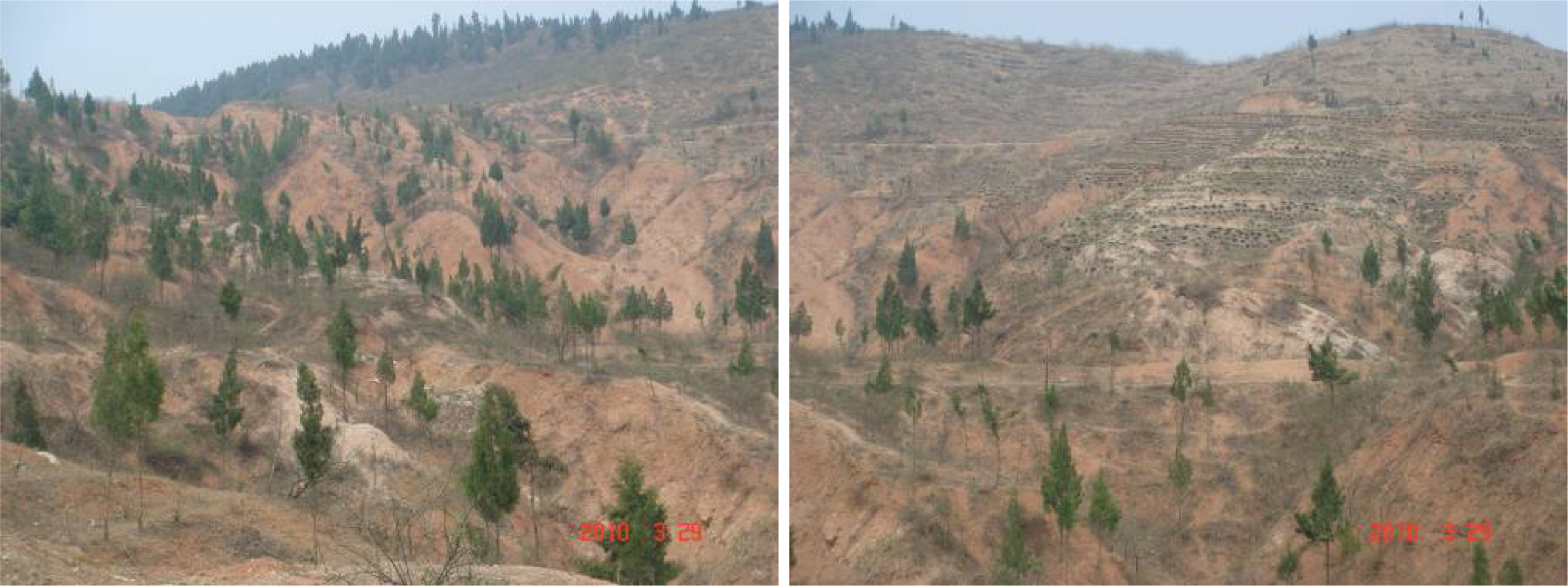
Figure 7b) were assessed by grading the vegetation fraction cover and slope gradient datasets according to the classification indices of the erosion risk for all land-use types, except for water body and construction land. The erosion risk field samples (
Figure 8) were random selected and the erosion status and intensity were judged mainly based on expert’s knowledge. By comparing the erosion risk field samples with the assessed erosion risk of 2010, the overall accuracy is 93%.
3.2. Comparison of Soil Erosion Risk
Trends in the overall erosion risk and erosion grade dynamic changes in time and space can be revealed by analysing the erosion grade in the same region with different phases. The spatial resolution of HJ-1B is similar to that of Landsat TM, and the spectral range is the same as the first four bands of Landsat TM. The acquisition dates of the 2004 and 2010 images are in June or May, which is the growing season of vegetation. Therefore, these two risk results are considered comparable. Trends in the overall erosion risk can be analysed in the macroscopic view by calculating the different erosion grade areas of two periods and by conducting a comparative analysis of the area dynamic change. The areas of each erosion risk grade of 2004 and 2010 are compared in
Table 3. The areas with erosion grades more severe than light are considered eroded.
The eroded area decreased from 5,751.04 km
2 (32.1% of the total study area) to 4,557.08 km
2 (25.43% of the total study area). The severe, more severe, and extremely severe areas decreased from 1,654.35 km
2 (9.23% of the total study area), 603.36 km
2 (3.37% of the total study area), and 142.92 km
2 (0.80% of the total study area) to 809.95 km
2 (4.52% of the total study area), 194.10 km
2 (1.08% of the total study area), and 32.85 km
2 (0.18% of the total study area), respectively. The light and moderate areas increased from 2,339.49 km
2 (13.05% of the total study area) and 3,350.41 km
2 (18.69% of the total study area) to 3,332.05 km
2 (18.51% of the total study area) and 3,520.18 km
2 (19.64% of the total study area), respectively. These findings suggest the overall decline in eroded area and the amelioration in erosion status. By overlaying the erosion risk results in 2004 and 2010 pixel by pixel, the percentages of each erosion grade transformation between 2004 and 2010 were obtained (
Table 4).
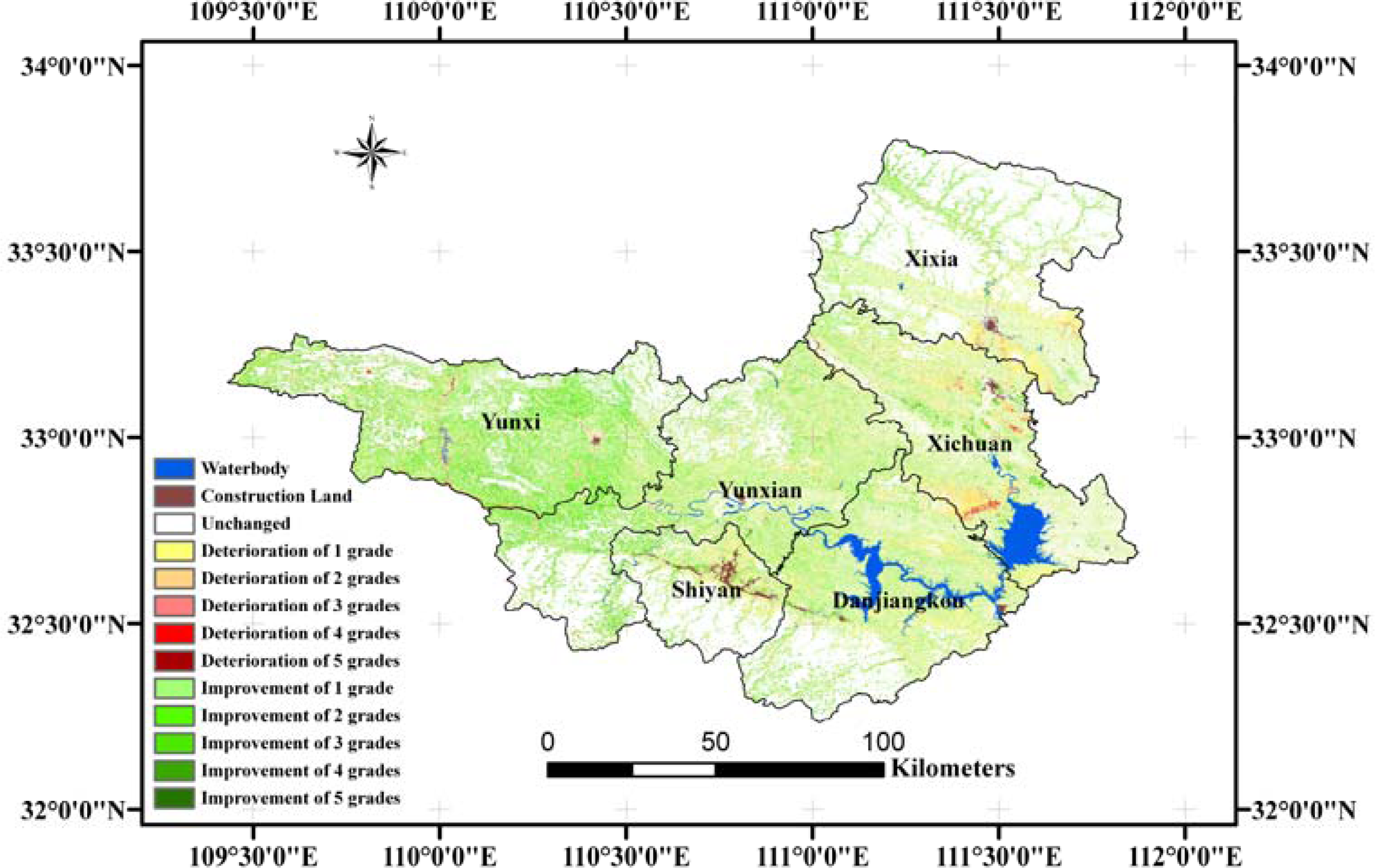
Table 4 shows the percentage of each erosion grade transformation between 2004 and 2010, and the sum of the diagonal value represents the percentage of unchanged regions account for the total area. The percentages of increase in erosion risk are above the diagonal and the percentages of decrease in erosion risk are below. As shown in
Table 4, the unchanged regions account for 54.81% of the total area. The deteriorative region accounting for 16.17% of the total area and improve region accounting for 25.92% of the total area. Consequently, the soil erosion situation overall is getting better. The areas of unchanged regions were greater at the lower erosion grades, indicating that areas with low erosion risk were more stable. Each row in
Table 4 represents the percentage of each erosion grade transformation from 2004 to 2010 account for the total area. For example, the first row in
Table 4 represents the percentage of “Slight” erosion grade transformation from 2004 to 2010 for the total area. The sum of the first row represents the percentage of slight erosion grade in 2004 for the total area, which is 54.81%. The “43.61%” represents that the erosion grade in 2004 and 2010 both are “Slight”, making up 43.61% of the total area. So, the percentage of unchanged “Slight” erosion grade in 2004 is 79.57%, equal divide 43.61% by 54.81%. The percentages of regions where erosion grade transformed from extremely severe to slight, light, and moderate were 0.18%, 0.02%, and 0.30%, respectively, and those of the regions where erosion grade transformed from slight to moderate, severe, more severe, and extremely severe were 4.03%, 0.54%, 0.16%, and 0.05%, respectively.
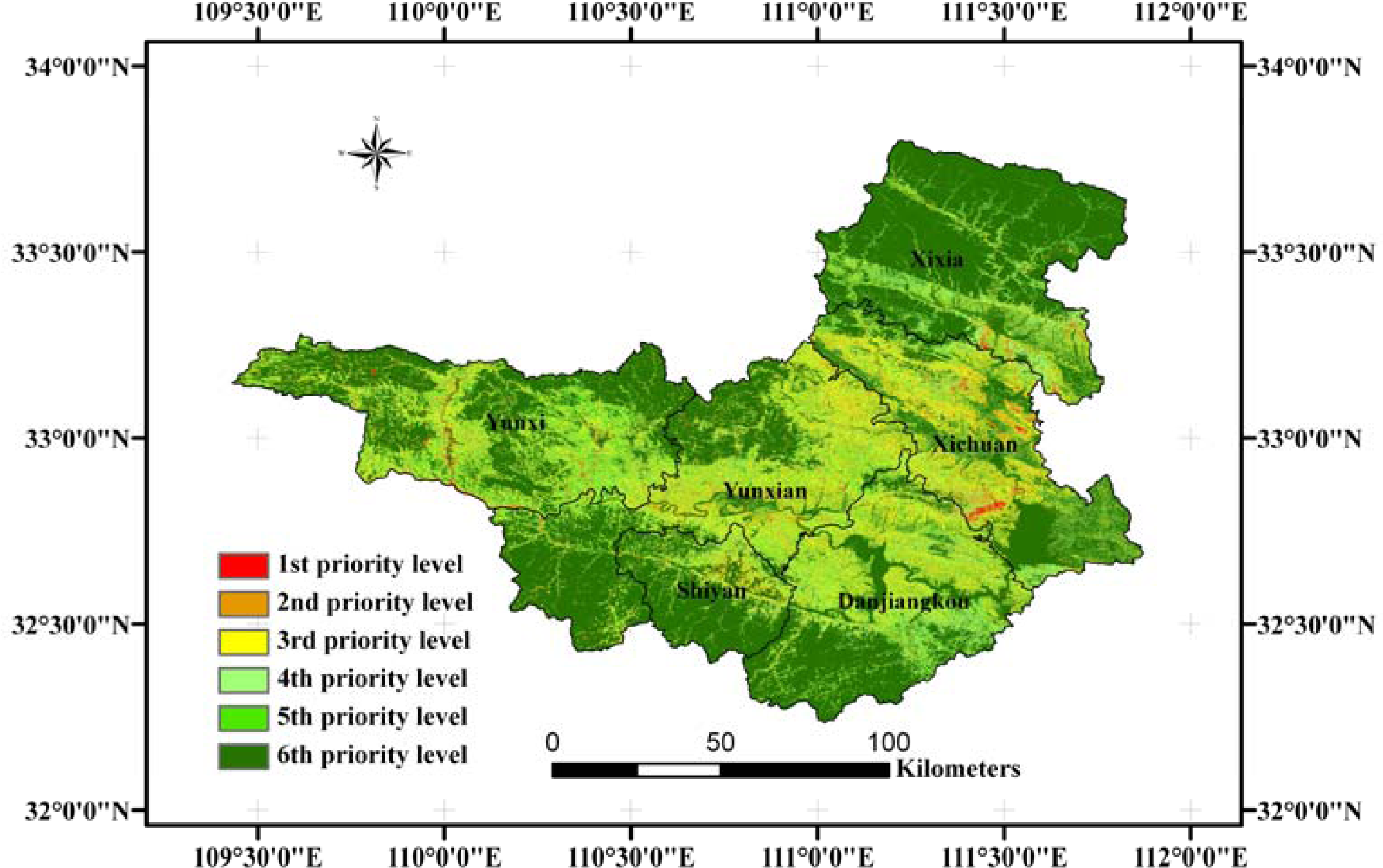
3.4. Regional Conservation Priorities
The determination of conservation priority of eroded regions is an important basis for the government in making decisions for soil and water conservation in the entire region. Each conservation priority indicates the urgent need for this eroded region to be managed. Consequently, the determination of conservation priority not only demands for considering erosion actuality but also erosion change trend. This study combines both current erosion risk and trends in erosion risk to determine conservation priorities. Accounting for changes in erosion risk means that regions with the same current erosion grade will not necessarily have the same conservation priority. For regions with unchanged erosion situations, the conservation priority is determined according to the erosion actuality. For the erosion situation of a deteriorated or improved region, the conservation priority is determined according to the trend of erosion deterioration or improvement. If the trend of erosion deterioration or improvement is obvious, the level of conservation priority of the region will be raised or reduced. Thus, multicriteria decision rules for identifying conservation priorities were set (
Table 6).
Based on the rules and erosion risk assessment results of the study area in 2004 and 2010, the conservation priority map was obtained (
Figure 10). The area of each level in the conservation priorities is shown in
Table 7.
Table 7 shows that the top two conservation priority levels cover almost all regions with severe erosion and prominent increase in erosion risk, with a total acreage of 1,309.76 km
2 and accounting for 7.31% of the study area. These two levels need to be managed as erosion control regions using appropriate conservation strategies in future projects. The third and fourth levels cover the regions with stable erosion status and slight change, accounting for 29.26% of the study area. These regions only need a minor allocation of funds for controlling soil erosion in future projects. The last two levels cover regions with low erosion grade and risk, with a total area of 11,369.17 km
2 and accounting for 63.43% of the study area. These regions need not be controlled for erosion as long as human activities are reduced and development intensity is rational.
4. Discussion
Soil erosion by water is the most important land degradation problem worldwide. The Danjiangkou reservoir area is the main water source and the submerged area of the Middle Route South-to-North Water Transfer Project of China. Soil erosion significantly influences the quality and transfer of the Danjiangkou reservoir water. The spatial distribution of soil erosion risk and the dynamic changes should be assessed to control soil erosion and protect the ecological environment. However, the research on soil erosion risk and trend analysis of erosion transformation in Danjiangkou reservoir area is rarely involved.
This study took two periods of remote sensing data by synthetically analysing the vegetation fraction cover, slope gradient, and land use. Although many factors influence water erosion, the vegetation fraction cover, slope gradient, and land use play an important role in affecting erosion resistance or risk. A multicriteria evaluation approach was also established for assessing erosion risk and monitoring changes in the trend of spatial distribution in erosion status and intensity between 2004 and 2010.
Compared with the Revised Soil Loss Equation (RUSLE) model which is considered to be a widely used approach of soil erosion assessment [
34,
36], the multicriteria evaluation approach does not directly consider the rainfall intensity and runoff as a factor, which is a drawback of this soil erosion model. Meanwhile, the RUSLE represents how climate, soil, topography, and land use affect rill and interrill soil erosion caused by raindrop impact and surface runoff [
60]. Concerning raindrop impact, the kinetic energy with which raindrops impact the soil surface and provoke detachment of soil particles depends on their velocity and size [
61]. However, the RUSLE is a model for predicting erosion which estimates long-term average annual soil erosion amounts [
62–
64]. It is applied to slope land, needs more accurate input data and has little consideration for the seasonal variation of vegetation. The RUSLE is likely to produce obvious errors to a specific rainfall and the region where the terrain is complex and the physiognomy type is diversified. In addition, in the case that the meteorological stations are of scarcity and uneven distribution, it is difficult to obtain the high resolution and accurate spatial distribution of precipitation data with raster format by spatial interpolation [
65]. Nevertheless, the risk assessment model in this study should include the rainfall intensity and runoff as a factor in the future.
There may be ecological function difference of the same vegetation fraction cover due to geographical differences. Relatively, the forest that had greater average age and higher average tree height and canopy density would have higher function of keeping water and soil. The water conservation function of evergreen broad-leaf forest is better than coniferous forest and the natural forest is superior to artificial pure forest. However, the land use variable in this study is limited to cultivated and non-cultivated areas. A better articulation among the different types of land use and related conservation management should be given further consideration.
The ground validation of remote sensing results is a complicated task. There needs to be a lot of ground-based measurements to assess the accuracy of remote sensing results in different eroded regions. In this study, the field samples were random selected and the erosion risk of samples were judged mainly based on experts’ knowledge, not based on the field measured data. It is a very simple validation method and the accuracy is more affected by experts’ subjective factors. Consequently, the ground validation of remote sensing results and the field assessment methods need further consideration in the future.
However, the key lies in the extraction of a valid vegetation cover and accurate land use. The assessment of erosion risk without a valid vegetation cover and accurate land use will produce inaccurate results and misguide the erosion control mission. An important limitation of this research is data availability and quality. The shortcomings of the datasets used in this study were that there was only two periods of remote sensing data with a six-year time span, and the dates of 2004 and 2010 images were not in the same season in a strict sense. In order to fully analyze the dynamic risk of soil erosion, more remote sensing data in the same growing season of vegetation with longer periods of time, higher resolution and cloudless conditions, should have been available. Where data are available, more distinct measures of trends in erosion risk can be obtained by analyzing the time series of erosion risks in a region, providing more detailed information to support conservation priorities.
5. Conclusions
By selecting Danjiangkou reservoir area, a vulnerable and sensitive ecological region, as the study area, this research synthesizes remote sensing and geographical information system techniques and analysing the vegetation fraction cover, slope gradient, and land use. Then, a qualitative assessment approach was used to assess water erosion (rill and sheet erosion) risk and the dynamic change trend of spatial distribution in erosion status and intensity between 2004 and 2010.
This research demonstrates the multicriteria evaluation approach could rapid and effective measure the probability and magnitude of water erosion risk and change trend over a large area. The changes in erosion intensity can be detected by the comparison of soil erosion risk in different periods. This study result shows the eroded area decreased from 32.1% in 2004 to 25.43% in 2010 of the total study area, suggesting an improvement in erosion status. The severe, more severe, and extremely severe areas decreased 4.71%, 2.28%, and 0.61% of the total study area, respectively. The results also indicate that the unchanged regions dominated the study area and that the total area of improvement grade erosion was larger than that of deterioration grade erosion. The percentages of regions where erosion grade transformed from extremely severe to slight, light and moderate were 0.18%, 0.02%, and 0.30%, respectively. The percentages of regions where erosion grade transformed from light to moderate, severe, more severe, and extremely severe were 4.03%, 0.54%, 0.16%, and 0.05%, respectively. The regions where erosion risk increased were mainly located in barren mountains, open forest land, young plantation land, and bare soil caused by development projects in the construction stage at which vegetation coverage was low. The regions where risk declined were mainly distributed in remote mountains with high vegetation coverage, where human activities were infrequent and vegetation coverage was high.
The soil erosion situation has improved in recent years through the measures taken up by the local government. These measures include the slope cultivated land below 15° being turned into terraced fields and the slope cultivated land between 15° and 35° being turned into orchards. The decrease in soil erosion risk and the reduction of eroded area from 2004–2010 show that soil erosion risk can be reduced by increased vegetation cover or the conversion of slope farmland to terraced field or orchards. To ensure the long-term development of the Danjiangkou reservoir, the government should continue to improve the management of slope cultivated land and the measures of changing farmland back to forest and closing hill sides to facilitate afforestation.
A conservation priority map was constructed based on the rules and on the erosion risk assessment results of the study area in 2004 and 2010. The conservation priority levels are important in water and soil conservation management and eco-environment improvement planning in the reservoir area in the future. The location and size of erosion control regions will be given more attention. The top two conservation priority levels cover almost all regions with severe erosion and prominent increase in erosion risk, accounting for 7.31% of the study area. The erosion risk and the dynamic changes trend results can provide guidance in developing and implementing water conservation planning and assist government agencies in determining the erosion control area, initiating regulation projects, and taking soil conservation measures.


