Assessing Regional Climate and Local Landcover Impacts on Vegetation with Remote Sensing

Abstract
: Landcover change alters not only the surface landscape but also regional carbon and water cycling. The objective of this study was to assess the potential impacts of landcover change across the Kansas River Basin (KRB) by comparing local microclimatic impacts and regional scale climate influences. This was done using a 25-year time series of Normalized Difference Vegetation Index (NDVI) and precipitation (PPT) data analyzed using multi-resolution information theory metrics. Results showed both entropy of PPT and NDVI varied along a pronounced PPT gradient. The scalewise relative entropy of NDVI was the most informative at the annual scale, while for PPT the scalewise relative entropy varied temporally and by landcover type. The relative entropy of NDVI and PPT as a function of landcover showed the most information at the 512-day scale for all landcover types, implying different landcover types had the same response across the entire KRB. This implies that land use decisions may dramatically alter the local time scales of responses to global climate change. Additionally, altering land cover (e.g., for biofuel production) may impact ecosystem functioning at local to regional scales and these impacts must be considered for accurately assessing future implications of climate change.1. Introduction
Vegetation is a key variable of interaction between the land and atmosphere. Driven by climate, vegetation is highly sensitive to precipitation and/or temperature, which depends on the region under consideration [1,2]. The central US Great Plains are a leading producer of wheat, sorghum and a significant amount of corn and soybeans. Production of corn for ethanol can reduce petroleum use by about 95% on an energetic basis [3]. However, food production and energy needs are competing pressures that alter decisions concerning the type of crops to produce. These landcover changes will have spatially and temporally varying environmental impacts, such as altering water cycling in this region. Understanding these impacts is vitally important for quantifying the responses to climate change in this major agricultural producing region.
For semi-arid regions, such as the central US Great Plains, biosphere-atmosphere interactions are strongly coupled to climate variability in these water-limited areas [2]. Precipitation is a primary control of vegetation dynamics in grasslands, and disturbances in both the frequency and timing result in observable ecosystem responses [1,4]. In addition, the structure and productivity of grasslands vary along different spatial and temporal scales of precipitation. Sala et al. [5] confirmed the importance of precipitation in relation to spatial and inter-annual variations in grassland production at a regional scale. It is known that long-term average precipitation can determine large-scale ecosystem and species distributions [6]. However, Yang [7] showed that the summer and spring precipitation was the dominant climate control on grassland productivity of the central and northern US Great Plains. Therefore, the variability in precipitation, across spatial and temporal scales, can strongly influence ecosystem dynamics [8], and ecosystems are very susceptible to climate change induced perturbations. Global circulation models are forecasting drying in the region is due to climate change [9], thus necessitating an enhanced understanding of ecosystem feedbacks between local land cover and regional climate for mitigating climate change.
The evidence for biotic responses to climate changes can be based on analysis of satellite data, and the Normalized Difference Vegetation Index (NDVI) is the most common indicator of terrestrial vegetation productivity [10,11]. NDVI can be used to evaluate responses of vegetation to climate change because it is well correlated with the fraction of photosynthetically active radiation (FPAR) absorbed by plant canopies and thus leaf area, leaf biomass, and potential photosynthesis [12]. Notaro et al. [13] also suggested that there is the largest interannual variability with large anomalies in the relationship between FPAR and precipitation on the prairie of the central US. Lotsch et al. [8] used continental scale precipitation data and NDVI, indicated that variability in precipitation at seasonal and longer time scales strongly influence ecosystem dynamics in arid and semi-arid regions, and illustrated the global extent and sensitivity of ecosystems susceptible to climate change-induced perturbations in precipitation regimes. In addition, Wang et al. [14] used NDVI to show that vegetation can influence climate variability through land-atmosphere interactions over semi-arid grasslands. In general, these results indicate there is a complex relationship between vegetation and precipitation or other climate forcings, which are highly variable in time and space [15].
The conversion of grassland to croplands and pastures has affected the exchanges of energy, water, and carbon, as well as ecosystem condition and function [16,17]. Not only does the vegetation-precipitation relationship vary in time and space, but it is also influenced by local landcover and land management strategies. For example, there is a significantly different development and spatial distribution of land cover and land use between eastern and western Kansas: eastern Kansas has a trend toward increasing urbanization and increased woody encroachment [18], while in the western portion of the state the dominant land use is agriculture, with a significant portion being irrigated [19]. These changes alter not only the surface landscape but also regional water cycling. Under global warming conditions, the environment may have significant responses to these hydrological changes caused by landcover; moreover, feedbacks between landcover and the water cycle will also be influenced by many other factors (i.e., urbanization, grazing, cropping, irrigation, etc.) across the region. Predicting the suitability of different regions to agricultural production will depend upon the accurate determination of local versus regional controls on the water balance.
In concert with the relationship between precipitation (or other climate forcings) and vegetation, many studies have used correlation analysis to examine how vegetation responds to climatic variables (i.e., precipitation, temperature) in different temporal or spatial scales [20–22]. However, in order to further characterize the interactions among vegetation and climatic variables, it is also important to understand the variability of climatic variables in the hydrologic and energy cycles. For example, Mishra et al. [23] employed an entropy-based investigation to quantify spatial and temporal variability/disorder of precipitation in Texas. The authors indicated entropy is a desirable approach to study the variability of precipitation based on the whole to part concept. Moreover, information theory has been used widely in applications of assessing hydrological variability, such as the scaling behavior both in space and in time [24]. Brunsell and Young [25] used the multiscale information theory metrics to examine the interaction between precipitation forcing events and land surface (NDVI and surface temperature) response, and concluded this method can determine the relative impacts of regional climate and local land-atmosphere interactions as a function of spatial scale.
Our proposed methodology, multiscale information theory metrics, which have been developed by Brunsell and Young [25], Brunsell [26] and Brunsell and Anderson [27], is a set of metrics to assess the spatial and temporal variability of hydrological processes and is able to be applied to land-surface hydrology and ecology [26]. As discussed by Stoy et al. [28] this method can quantify the appropriate scales for observations and modeling studies. Besides, entropy could aid in distinguishing different spatial patterns by applying it to hourly precipitation [29] and improving short-term precipitation forecasts [30]. It was also used by Brunsell and Young [25], who assessed the spatial and temporal interactions between precipitation, soil moisture and vegetation dynamics and indicated that the multiscale information theory could address the wide range of spatial and temporal scales that contribute to the observed data.
Therefore, the motivating objective of this study is to examine the relationship between vegetation productivity and the roles of local land cover type and regional climate (i.e., precipitation). Specifically, the major objectives are first, to understand the temporal dynamics associated with different landcover types as a function of location along the mean precipitation gradient and, second, to assess to what extent are different longitudes within the KRB governed by microclimatic impacts (i.e., landcover) or climate forcing (i.e., PPT).
2. Study Area and Data Sources
2.1. Study Area
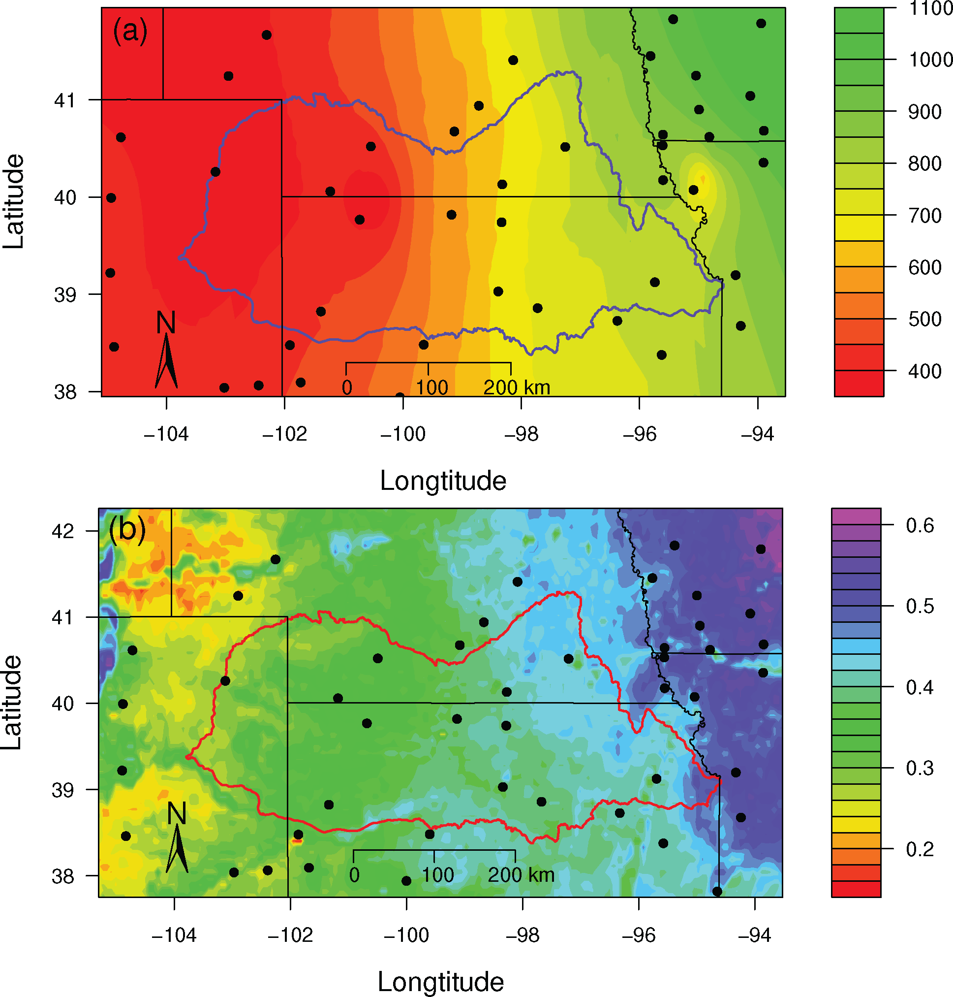
The central US is an area of significant agricultural production, and for this study we focus on the Kansas River Basin (KRB), which is located in northern Kansas and extends into southern Nebraska and a portion of eastern Colorado (Figure 1). Across the KRB, there is a profound precipitation gradient extending from dry in the west (400 mm/yr) to moist in the east (1,000 mm/yr) [31]. The current ecosystems are highly influenced by local land use management strategies including balancing the increasing demand of food and biofuel production, which will extend potential impacts of the environmental changes, both in the native and agricultural lands. Most parts of the KRB are agricultural and prairie. Short-grass prairie is in the west, mixed prairie is in the center, and tall-grass prairie is in the east. By landcover type, croplands (40% of KRB) are primarily located in the central to west, grasslands (41% of KRB) are distributed primarily in the east, and woodlands or forests (4% of KRB) are only found as riparian along river valleys in the east [32]. It is an opportune area to address the questions of ecosystem dynamics changes through time, because unlike the top corn producing areas, land in the KRB is used for a wide variety of agricultural uses (i.e., corn, soybean, Conservation Reserve Program (CRP), grazing, etc.) as well as natural landcover types such as C3 and C4 grassland. This basin is likely to undergo changes from a significant number of landcover types as demand for one or two crops (i.e., corn and soy) increases. There are additional uses competing for land surface area including woody encroachment and urbanization.
2.2. Data Sources
2.2.1. NDVI
Currently, AVHRR is the best historical and the longest record of data for monitoring vegetation [33,34]. Twenty-five years (1982–2006) of AVHRR satellite data was used to examine vegetation dynamics as a function of land cover types (soybean, corn, and CRP lands, etc.). The Global Inventory Monitoring Modeling Studies (GIMMS) data set is a maximum 15-day composite NDVI product at 8-km spatial resolution available for a 26-year period spanning from 1981 to 2006, derived from AVHRR onboard the afternoon-viewing National Oceanic and Atmosphere Administration’s (NOAA) satellites series 7, 9, 11, 14, 16 and 17 [35].
2.2.2. Precipitation
Precipitation (PPT) was used as a measure of the regional climate variability because of the east-west gradient across the KRB [36]. The daily precipitation data is from the US Historical Climate Network (USHCN, [37]). Seventy-six stations across KRB transect were located from 93.5 to 105.5 W Longitude and 37.5 to 42 N Latitude (Figure 1a), and whose length of the observations records is the same as the period of NDVI (1982–2006). We aggregated the daily precipitation to 15-day totals in order to match the same temporal resolution of the NDVI data. Instead of comparing an individual station or a group of stations with the model output, we interpolated the precipitation to the latitudes and longitudes of these stations using kriging [9,38].
2.2.3. Land Use and Land Cover
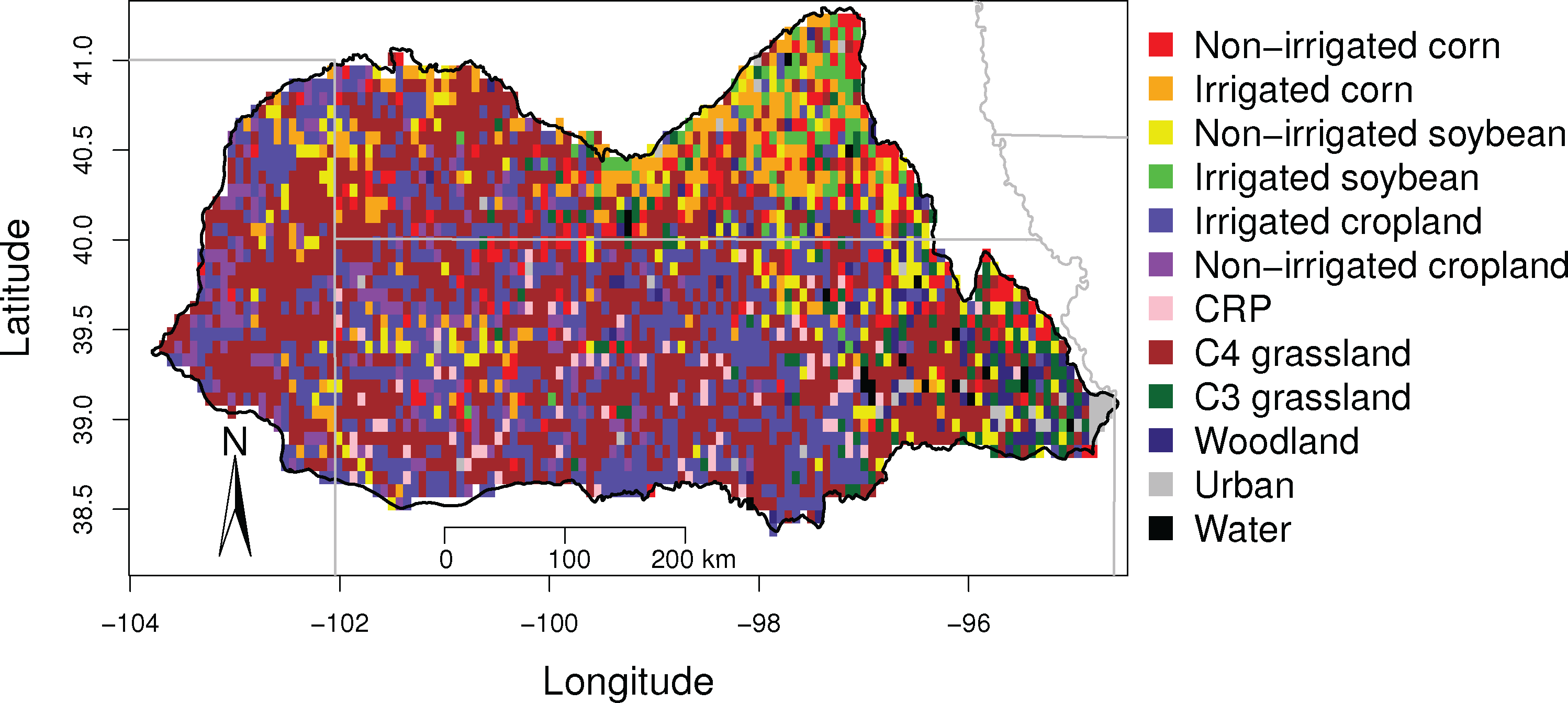
Despite variable crop cultivations in the central US over the time period of interest, the total factions remained fairly constant according the USDA [39] (e.g., corn varied between 22.1% and 22.6% of the KRB, while wheat varied between 20.4% and 21.4%) [40]. In order to assess the distribution of landcover across the KRB, we used the 24 class, 1-km spatial resolution 2005 Kansas Land Cover Patterns Level IV map, created by the Kansas Land Use/Land Cover Mapping Initiative [41]. We combined this with the agricultural statistics and published Green Reports [42], which defined different landcover types from the Advanced Very High Resolution Radiometer (AVHRR) based NDVI. For our purpose, we focused on specific landcover types, which contributed to both food and biofuel productions since those are the dominant landcover types. We aggregated this data to 12 primary landcover types, which are: irrigated corn, non-irrigated corn, irrigated soybean, non-irrigated soybean, irrigated cropland (including irrigated sorghum, winter wheat, alfalfa, fallow and double-crop), non-irrigated cropland, CRP land, C4 grassland, C3 grassland, woodland, urban, and water (Table 1). In addition, this landcover data was resampled to an 8-km grid to match the resolution of 8-km GIMMS NDVI data by using majority approach in the ArcGIS 9.1 software package (Figure 2).
3. Methodology
3.1. Wavelet Multi-Resolution Analysis
Wavelet analysis is a technique to view a data series as a function of different spatial and/or temporal resolutions, and each different resolution can be referred to be “a level of decomposition”. It allows for quantifying the variance contributed by each resolution and also determine when (temporally) or where (spatially) the contribution originates from [25]. Wavelet analysis has more benefits of taking both time and frequency into account. This is in comparison with a similar technique of Fourier transformation, since Fourier transformation only focuses on frequency and is not capable of characterizing a signal whose frequency content changes in time such as precipitation [43]. Previous studies such as Brunsell and Gillies [44] and Brunsell and Young [25] have applied wavelet analysis to assess the relationship between water and energy cycling and vegetation in terms of spatial variability and distribution. In this study, we followed the method of [27] and examined NDVI and PPT to ascertain temporal variabilities of the land surface and precipitation. We quantified the variability of precipitation and landcover as a function of temporal scale, and PPT and NDVI signals were compared at each level of decomposition. The wavelet transform (W(m,n)) in this study was conducted using the Daubechies least-symmetric 8 wavelet as a mother wavelet ψ to achieve a high level of localization in both time and frequency domains. This mother wavelet is then dilated (m) and translated (n) across a time-series f as a function of time t [45]:
The unique capability of wavelet multi-resolution analysis “zoom-in” allows the identification of local brief, high-frequency signal and low-frequency variability in a time series. Windows are able to look at different frequency signals: being wide for low-frequency while being narrow for high-frequency [46]. At each level of decomposition, the original signal (f (t)) can be reconstructed from the wavelet coefficients Dm,n as:
Wavelet multi-resolution analysis is a dyadic (powers of two) decomposition in scale, and we have chosen to conduct nine levels (corresponding to lengths of 2, 4, 8, 16, 32, 64, 128, 256, and 512) based on the length of the time series. By progressively adding the finer scale details, the original dataset X at scale m can be reconstructed from the inverse wavelet transform, using fluctuations (X′) at each point t:
In addition, we calculated the wavelet spectra as a function of time scale m to examine how much each decomposition level contributed to the overall signal, which are given by:
3.2. Information Theory Metrics
Information theory has been previously used to examine land-atmosphere interactions [25–27]. Entropy is a measure of the statistical uncertainty of the random field X as described by the probability density function (pdf). Lower entropy represents less uncertainty, which means the amount of information needed to encode the signal is smaller [47]. For this study, Shannon entropy (H) [48,49] is used as a measure of the spatial-temporal variability of precipitation and vegetation, which is defined as:
The relative entropy (R(X, Y)) is a measure of the distance between the two variables X and Y given by the pdfs p and q, respectively, and R(X, Y) is zero if they are the same [50,51]. For example, p is the pdf of NDVI (X), and q is the pdf of PPT (Y), and relative entropy can measure how much PPT tells us about NDVI (R(NDVI, PPT)) as well as how much NDVI tells us about PPT (R(PPT, NDVI)). Relative entropy is defined as:
There are two ways for computing the relative entropy for this study. In the first case, we computed the relative entropy between the original data and a decomposed version data from the wavelet multiresolution analysis. This was done to isolate the relative contributions of these timescales to the overall signal, e.g., computing the relative entropy between seasonal precipitation and total vegetation [26]. Therefore, we explicitly do not want to filter out temporal scales such as the annual or seasonal scales prior to computing the information theory metrics. Secondly, the relative entropy was computed between each decomposed scale of precipitation and NDVI. This part was for assessing how much additional information is necessary to represent the vegetation when given a particular scale of precipitation, and vice versa.
In order to compute the entropy and relative entropy of precipitation and NDVI, we first decomposed the time series of precipitation and NDVI signals using the wavelet multiresolution analysis described on the previous section. At each scale of decomposition, the pdf of the decomposed time series (X′m (t)) was calculated and then used to compute the Shannon entropy and the relative entropy as a function of temporal scale of decomposition.
4. Results
4.1. General Distribution of Surface-Atmosphere Interactions Across KRB
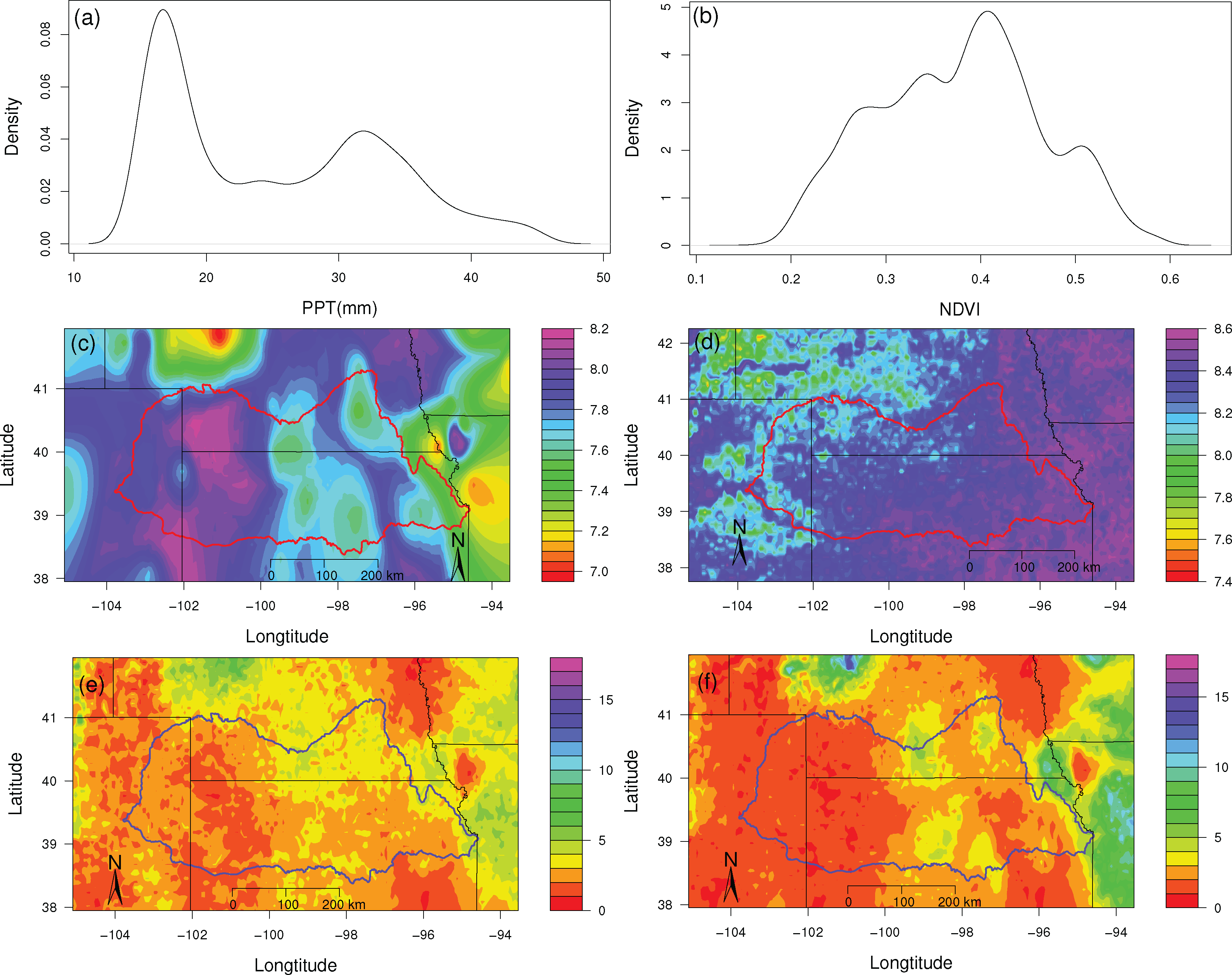
Spatial and temporal biosphere-atmosphere interactions, such as fluxes of water and energy, are strongly coupled to climate variability in grasslands [8]. Figure 1a shows the spatial distribution of averaged precipitation varies from dry in the west (approximately 400 mm/yr) to more moist in the east (up to 1,000 mm/yr). The distribution in the growing season (June, July and August) was generally the same as the annual precipitation and the amount was from about 90 mm/yr to 270 mm/yr, which contributed about one third of the annual amount.
Variations in climate factors, such as precipitation, have strong influences on the variation of NDVI for a given area. Figure 1b shows that the spatial distribution of mean annual NDVI generally corresponds to the precipitation. We also noted that along the west edge of the KRB, NDVI distribution followed the terrain.
Figure 3a,b presents the probability density functions of precipitation and NDVI, which were estimated using data from all grid points. They were used for calculating the entropy and relative entropy of precipitation and NDVI. The information theory analysis was applied to examine how the temporal information content of vegetation and precipitation varied over the KRB. The NDVI had more variance within the pdf than PPT and resulted in a higher entropy value (H(NDVI)=8.32, H(PPT)=7.75. The values are the average over the period of analysis and the KRB.). Figure 3c,d shows the spatial distributions of variability for PPT and NDVI (H(PPT) and H(NDVI)). The values of H(PPT) generally are higher in the west and lower in the east, however H(NDVI) gradually increased to the east across the basin. The increasing trend of H(NDVI) corresponds to the west-east trend of mean annual NDVI, which notes the longitudinal change in vegetation is determined by the dynamics of landcover types.
The maps of the relative entropy between PPT and NDVI are shown in Figure 3e,f. R(NDVI, PPT) illustrates how much additional information is necessary to represent vegetation given by precipitation; and R(PPT, NDVI) indicates the reverse. Both relative entropies showed the same general variability, where lower values exhibited in the west and increased to the east. R(NDVI, PPT) showed a clear break at around 100 W longitude, however R(PPT, NDVI) did not have this spatial trend. This break also demonstrates that the variability of landcover corresponds to the precipitation gradient, as well as the increase in irrigation in the western part of the KRB. Besides, the further western part indicates a tightly coupled relationship between the precipitation and vegetation until the annual amount of PPT reaches 600 mm/year (around 101 W) and then this relationship decouples as the amount of PPT increases.
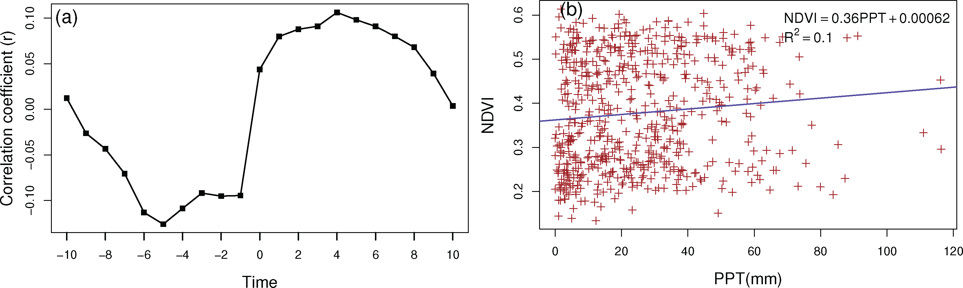
We compared the proposed method and metrics with other traditional statistical analysis as well. First is the correlation analysis: we examined the relationship between NDVI and different time lags of PPT by calculating correlation coefficients between NDVI of the various periods and corresponding precipitation (e.g., current period of NDVI and previous period PPT). However, the results did not show any significant correlation between NDVI-PPT within KRB (−0.1 < r < 0.1, Figure 4a). Secondly, we have tested if NDVI and PPT exhibited non-stationarity during the study period by linear regression analysis. Again the results had a weak relationship between NDVI and PPT (r2 = 0.1), shown in Figure 4b with the correlation between 15-day composited NDVI and 15-day totals PPT over the 25 years.
4.2. Distribution of Landcover Types
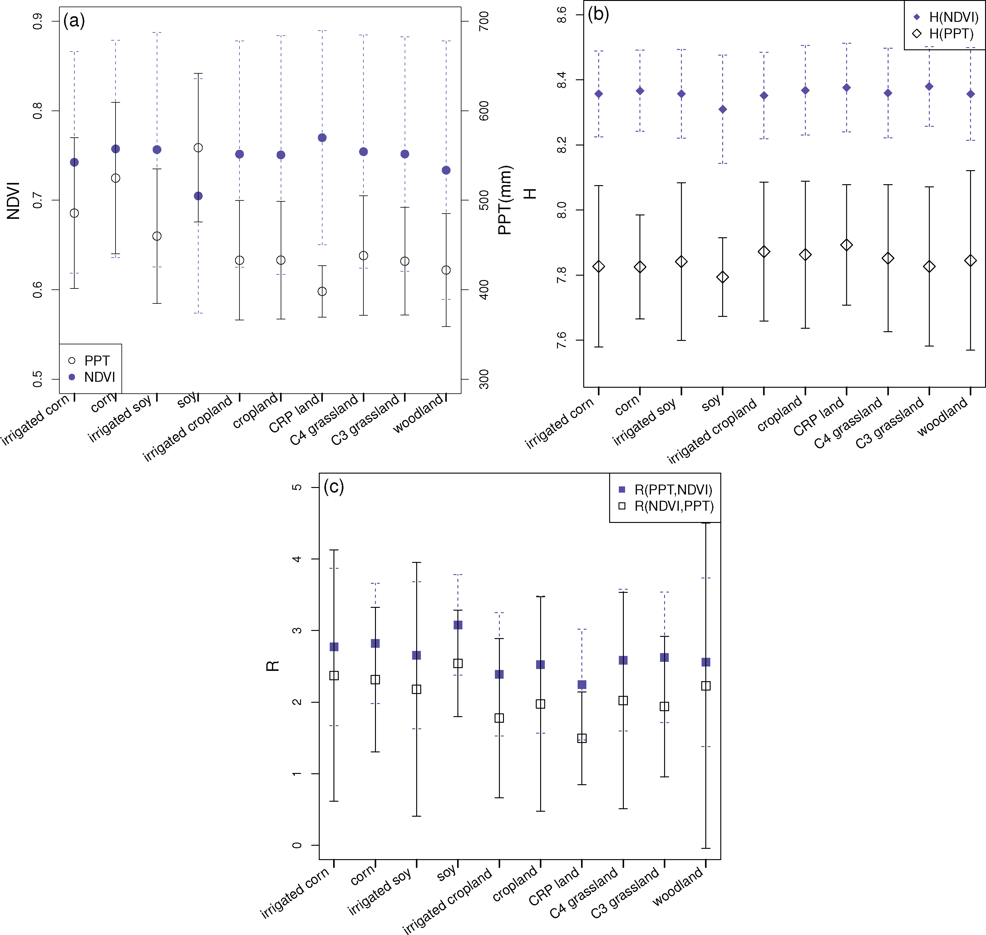
In addition to the gradients of vegetation and precipitation across KRB, we examined the spatial-temporal distributions within each landcover type (Figure 5a). In order to clearly distinguish NDVI values among ten landcover types, we used the maximum NDVI to show the relationship between landcover types and precipitation. Generally, high NDVI values corresponded to high PPT, with soybean and CRP land being two noticeable exceptions. Among these landcover types, the maximum NDVI value of each landcover type was slightly different, while the difference in the annual precipitation for each landcover type was up to 137 mm. This contrast between NDVI and PPT illustrates that irrigation management leads to vegetation productivity independent of the larger scale precipitation gradient. Non-irrigated landcover types are primarily located in the more mesic eastern region, whereas irrigated land use dominates in the more arid west.
We examined the variability of the entropy of PPT and NDVI as a function of landcover type (Figure 5b). The variability showed a similar distribution as NDVI for each landcover type compared with Figure 5a, but did not present as much difference among landcover types with reduced standard deviation of entropy in NDVI spectra for each type. H(PPT) slightly varied by landcover as well. We also calculated how much of the information in the vegetation distribution was related to the precipitation variability within each landcover type (Figure 5c). Clearly the R(NDVI, PPT) values of ten landcover types were all lower than R(PPT, NDVI), which implies less additional information is needed to represent vegetation by the given precipitation rather than predict the PPT from the NDVI. Fluctuations of R(PPT, NDVI) and R(NDVI, PPT) among all landcover types were also approximately equal.
4.3. Temporal Structure of Precipitation and Vegetation
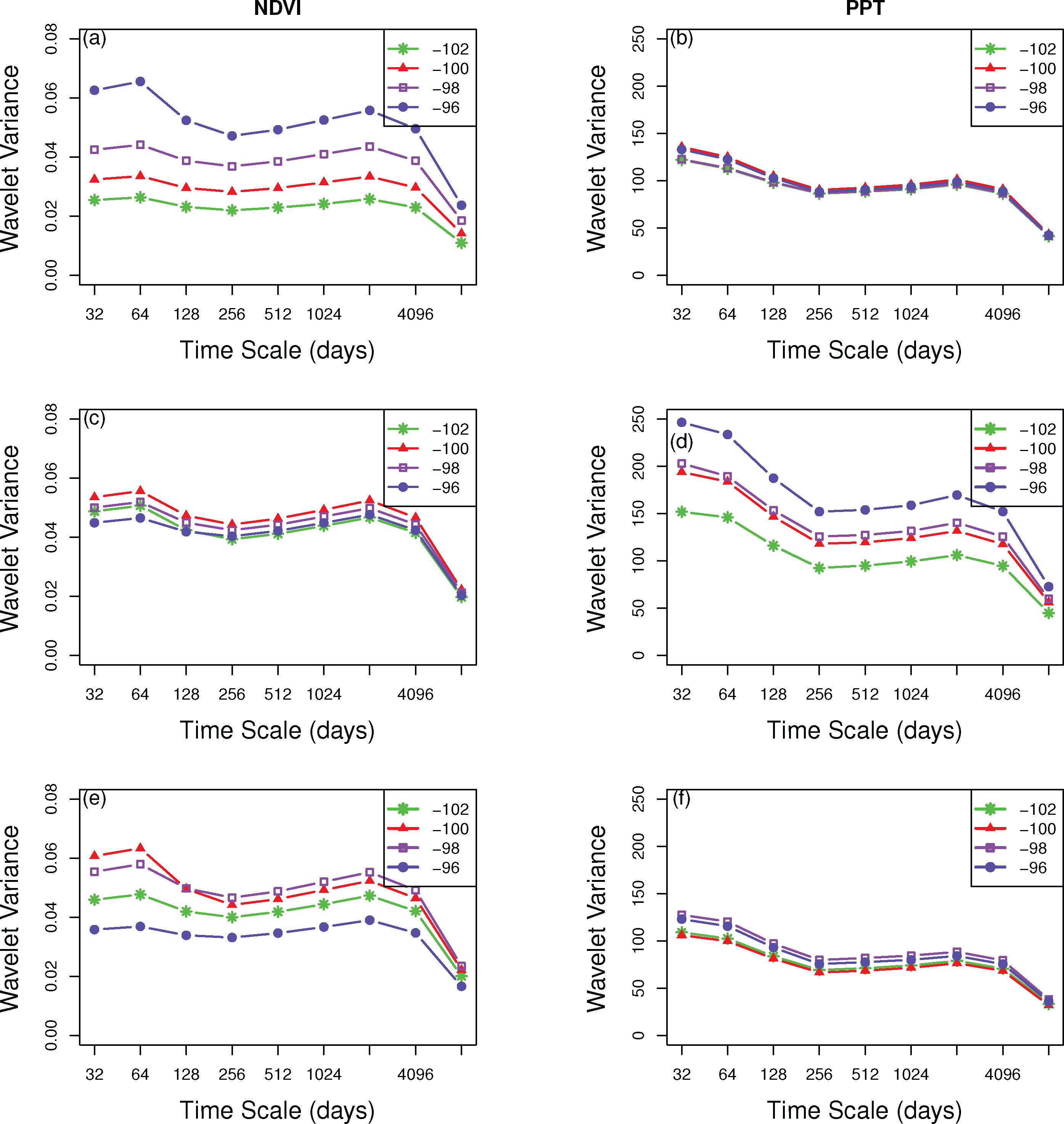
We calculated the wavelet spectra to quantify how much variance of PPT and NDVI is contributed by different temporal scales. This was conducted at selected longitudes along the KRB and as a function of landcover type.
Figure 6a shows that for NDVI there were clear variations in the peaks in the wavelet spectra as a function of longitude. For entire KRB signals, the overall wavelet variance was highest at 96 W, while the other longitudes showed approximately the same curves but variances decreased from 98 W to 102 W, which could reflect less heterogeneity in the western part of region. The dominant time scale (largest peak) of 96 W was on the scale of 64-day. However, at the other longitudes they did not exhibit this peak.
Differences in landcover types induce minor variations across longitudes. Due to managed irrigation, irrigated corn (Figure 6c) exhibited almost the same curves across KRB with a slight peak at the 64-day scale. For C4 grassland (Figure 6e), the peak was at the same scale as the entire basin (64-day) but longitudes exhibited different order of magnitudes of variance.
Precipitation within the KRB (Figure 6b) showed the dominant scale was at the monthly scale, which surprising did not vary across longitudes. Moreover, in this monthly scale, irrigated corn variances were increasing as a function of easterly position along the gradient (Figure 6d). For C4 grassland (Figure 6f), there were also west-east increasing variances though much less distinct (in magnitude) than irrigated corn.
4.4. Multi-Resolution Entropy Metrics of Precipitation and Vegetation
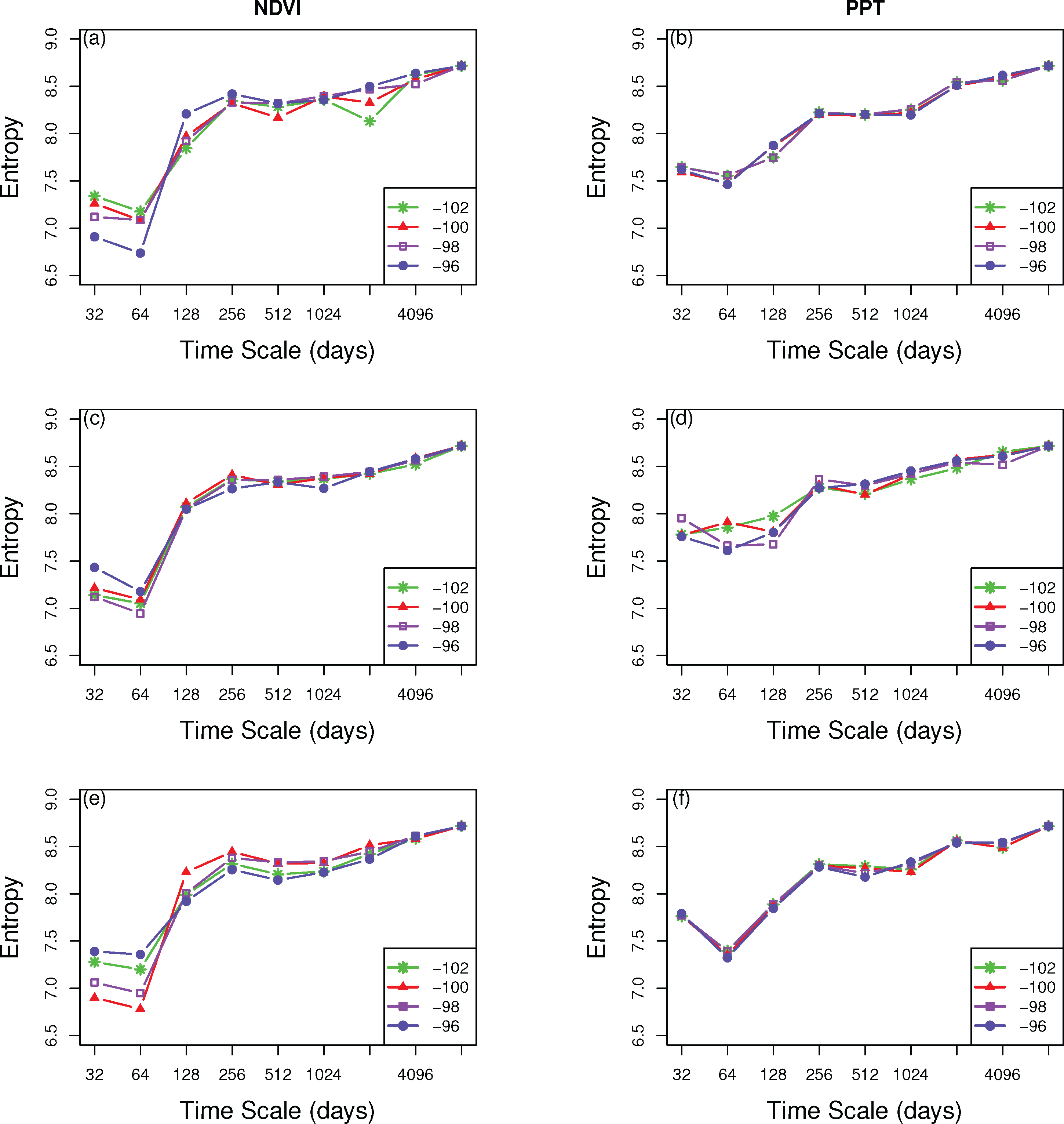
Next, we conducted a wavelet multi-resolution analysis to calculate the multiscale entropy for the PPT and NDVI. The general behavior was increasing entropy with increasing time-scale. The marked increase of NDVI was in the 128-day (seasonal) scale and slowly went up through longer time-scales. More variance was found up to the seasonal scale for the entire basin and selected landcover types (irrigated corn and C4 grassland). Within the seasonal scale for the entire basin (Figure 7a), NDVI spectra showed that there was a decreasing trend from west to east. Irrigated corn varied more in the east region (96 W) (Figure 7c), while C4 grassland in the far west and east regions exhibited less variation than the central part (Figure 7e).
The entropy of PPT had the greatest increasing trend at the 512-day time scale. This increasing trend was consistent across the entire KRB (Figure 7b), with slight variances at 64-day (bimonthly) and 128-day (seasonal) time scales. The same distribution was seen in C4 grassland (Figure 7f), however few differences between longitudes were observed, except at the 512-day and 1024-day time scales. Irrigated corn illustrated more fluctuations among longitudes at shorter time-scales and then converged at the 512-day scale (Figure 7d). In addition, the distribution of woodland was a good example to indicate differences between west and east because of similar behaviors at both 98 W and 96 W, which matched the distributions of irrigated corn and C4 grassland at the eastern region (not shown).
4.5. Multi-Resolution Relative Entropy of Precipitation and Vegetation
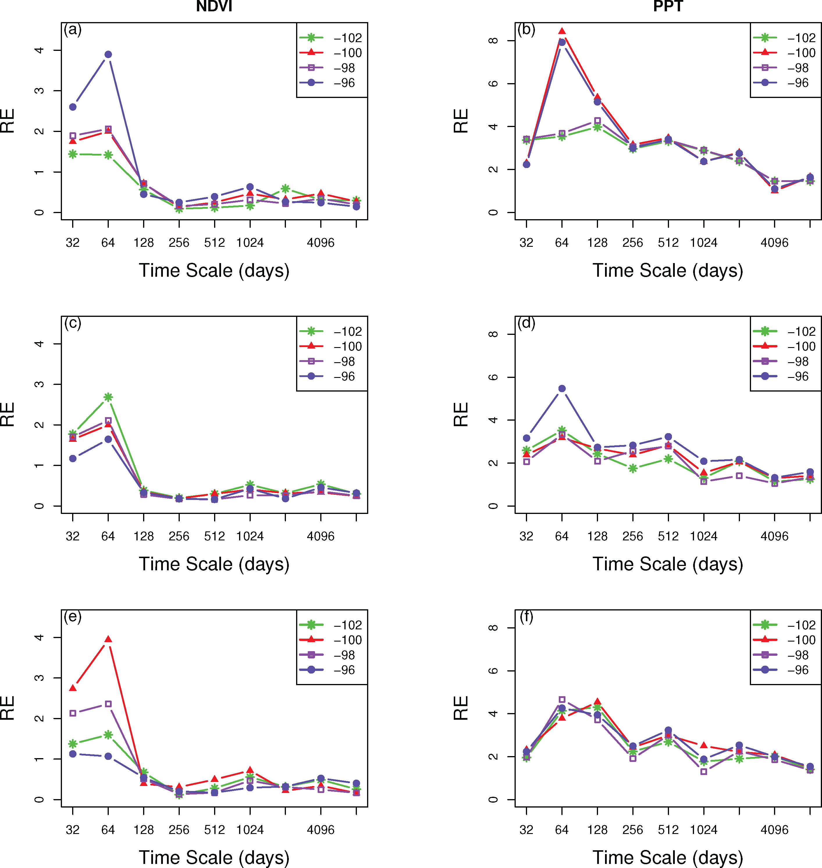
In order to determine how much information is contributed to the total signal of PPT and NDVI by certain time scales, we calculated the relative entropy between the original PPT and NDVI and decomposed PPT and NDVI at each individual scale. For the entire KRB (Figure 8a), the relative entropy between NDVI and its decomposed version showed that higher values and variations across longitudes were at shorter (monthly and bi-monthly) time scales, while smaller, approximately constant values were at time scales greater than the 256-day. Similar distributions of spectra were found in the different landcover types. For irrigated corn (Figure 8c), a clear variation of westerly information was seen at the shorter time-scales. C4 grassland (Figure 8e) also showed higher values at the shortest time scales, but there was no consistent variation with longitude. This implies that at monthly and bi-monthly scales NDVI contained less information about the total signal of NDVI, while the annual scale was the one that was contributed the highest amount.
The results of PPT for the entire KRB showed reduced values with increasing time scale with a particularly high R value at 96 W and 100 W at the bi-monthly scale (Figure 8b). However, different landcover types showed variation across scales in the multi-scale relative entropy. Irrigated corn (Figure 8d) showed relative entropy values approximately twice as large in eastern region of KRB (96 W) at the 64-day (bi-monthly) time-scale. The other longitudes varied with different temporal scales, with perhaps a slight reduction with increasing time scale. The C4 grassland exhibited similar variation across longitudes (Figure 8f): the eastern part (96 W and 98 W) exhibited the highest peak at 64-day (bi-monthly) time-scale while the western part (100 W and 102 W) showed a peak at 128-day (seasonal) time-scale. These peaks indicated that these scales were particularly less informative in comparison with other time scales. Generally, the relative entropy for the individual landcover type varied more at relatively shorter time scales. These results illustrated how different land cover types from west to east along the precipitation gradient respond to climate forcing as shown in the results of multi-resolution entropy.
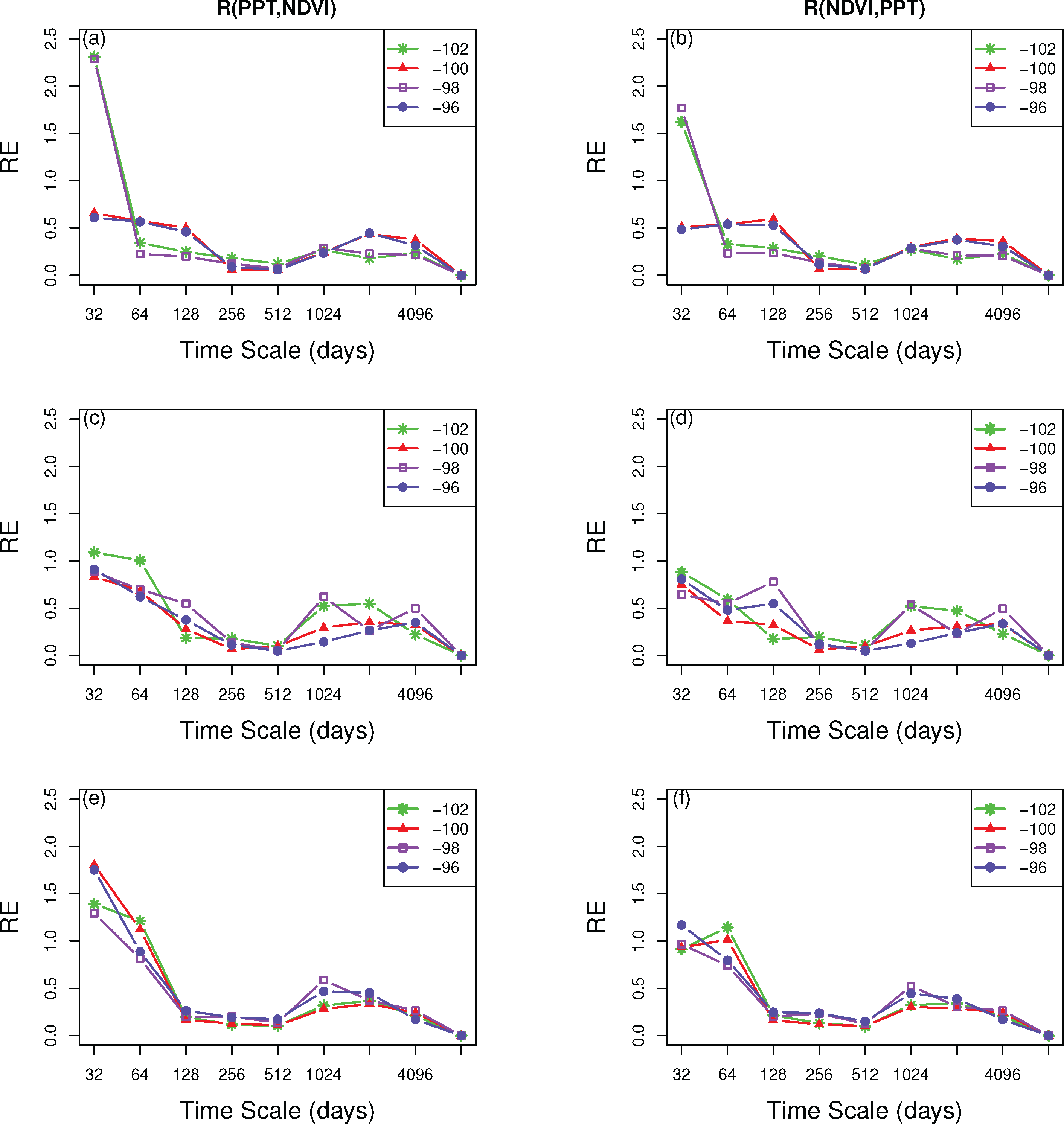
In addition, we also calculated the relative entropy between NDVI and PPT as a function of scale to examine how informative different time scales of the PPT signal were at determining the NDVI data and vice versa. The results of R(PPT, NDVI) showed that the 32-day (monthly) scale was contributed the least information (had the highest R value). Two distributions were noted across the basin (Figure 9a): (1) at 98 W and 102 W, there were really high R values at the 32-day (monthly) time-scale and decreased as a function of time scale; (2) two peaks showed at 32-day and 2,048-day time-scale, at 96 W and 100 W, respectively. Longitudinal distributions of irrigated corn (Figure 9c) were approximately the same but not consistent at the 64-day (bi-monthly) time scale and longer time-scales. Irrigated corn also showed slightly higher R(PPT, NDVI) at the 256-day and 1,024-day time scales. C4 grassland looked similar across the whole basin (Figure 9e) with higher values in 32-day (monthly) and 64-day (bi-monthly) time scales.
The distributions of R(NDVI, PPT) for the whole KRB were almost the same as the results of R(PPT, NDVI) (Figure 9b), with only reduced values on the monthly time scale at 98 W and 102 W. With regard to the individual land cover type, the highest value was at the shortest (monthly) time scale and showed little variation across longitude. For irrigated corn (Figure 9d), there was clear variation by longitude (except 96 W) at the seasonal time scale. C4 grassland (Figure 9f) was relatively constant across all time scales but had a slight variation at the bi-monthly time-scale.
5. Discussion
Climatic controls are the primary influence on grasslands with the possible exception of irrigation [8]. The relationship between vegetation and climate variables is generally obvious but is highly variable in time and space. The spatial distribution of vegetation generally corresponded to the precipitation increase (Figure 1).
Compared with the proposed method and metrics, other traditional statistical analysis like the correlation analysis and linear regression analysis have shown no significant results. This agrees with a study of the assessment of spatial-temporal variability of daily precipitation across the continent [26], which had almost identical spectra across all longitudes and therefore concluded that correlation may not be a useful metric for assessing the spatial or temporal variability of precipitation. Besides, this non-significant relationship also demonstrated that other factors, such as soil moisture and soil reflectivity may have an influence on the vegetation response [52].
As the information theory metrics used in this study are qualitative rather than quantitative, and are computed at each time scale from the estimated pdfs, the values of entropy and relative entropy are conveniently used to interpret the variability of precipitation and vegetation.
Entropy metrics can show the spatial gradient of precipitation and vegetation (Figure 3c,d) and moreover be able to assess their temporal/spatial variability. The higher H(PPT) was in the western part of KRB, and this high variation could indicate that some extreme events such as drought happened during the study period. This agrees with a study in Texas [23] where disorder in precipitation amount and a strong spatial gradient of rainfall days might relate to significant historical drought periods. Since vegetation was largely impacted by precipitation, lower H(NDVI) in the western KRB indicated only drought tolerant land cover types (e.g., C4 grassland) could adapt to this varied climate condition; while with increasing PPT, landcover becomes more diversified to the east. Relative entropy is another useful means for our study to assess the amount of additional information that is needed to represent vegetation given PPT or vice versa. In Figure 3f, different amounts of information of PPT were needed to represent vegetation. The precipitation and vegetation dynamics were tightly coupled until mean annual PPT reached approximately 600 mm/year (at 100 W) with decreased coupling occurring with increased PPT.
One objective of this study was to understand the temporal dynamics associated with different landcover types as a function of location along the mean precipitation gradient. Overall, regional precipitation was the main control for vegetation, and can be a good predictor of vegetation productivity [1], shown in Figure 1b. Though vegetation changes all corresponded with the regional precipitation gradient, they showed different levels of tightness with precipitation. (Figure 5c). Meanwhile, the impact of varying different landcover types has been clearly shown in the comparison of entropy of PPT between irrigated corn and C4 grassland at 102 W ((Figures 7d,f). The results of their different spectra at the bi-monthly time scale conclude that grassland corresponded to precipitation more than cropland in the KRB. However, as we have noted that among landcover types there was not much difference, so the issue of misclassification in the landcover dataset due to sub-pixel heterogeneity that could impact our results may need to be considered. The changes among landcover types in the KRB followed a seasonal cycle (Figure 8a,c,e), which was also found by Yang [7] who concluded that seasonal precipitation, not annual rainfall, was the dominant control for vegetation. In addition, the temporal dynamics of vegetation varied not only by landcover types but also by location along the precipitation gradient. For natural landcover, such as C4 grassland and woodland (not shown), changes followed the seasonal cycle, which appeared in the center of the precipitation gradient. However, no obvious cycle was found in the moistest (east) area (Figure 6e), which may imply less response to climate forcing. The same results existed in irrigated corn across longitudes (Figure 7c). Due to different microclimatic conditions (i.e., soil moisture, topography, land management, etc.), the same landcover type in different locations along the precipitation gradient contained similar amounts of information at different scales. This was also observed in other landcover classes, e.g., non-irrigated soybean.
Next we examined how different longitudes within the KRB were governed by microclimatic impacts (i.e., landcover) or climate forcing (i.e., PPT). Vegetation in the KRB was affected by the local environment as indicated by diverse landcover types, though PPT was the main control for vegetation. It was evidenced at some locations in the western portion (shown in a range between 102 W and 100 W) of the KRB by having relatively same NDVI values (Figure 1b), but also an obvious precipitation gradient (range was from 450 mm to 650 mm). This indicates the presence of large-scale irrigation, mentioned in the study of the impact of irrigation on the US High Plains [19]. Rain-fed corn areas have been converted to irrigation (about 60% of the total corn producing area) and also show a cooling effect that causes a decreasing trend in mean and maximum air temperature in the irrigated region. Furthermore, even though the general west-to-east increasing trend in vegetation is a function of location along the precipitation gradient, local vegetation does not always match this distribution. Figure 6c has presented the variance of the mean NDVI of irrigated corn that was approximately the same across the entire basin, presumably due to the fact that the water deficit is offset by the increase in irrigation.
The distribution of land cover in KRB clearly indicated the impact of the local microclimate. Irrigated landcover types i.e., irrigated corn, soybean and cropland had approximately the same NDVI values (Figure 5a), but they were located in different portions of the KRB; corn was located in the western part of KRB while soybean was in the central KRB. Based on their locations, soybean generally received more precipitation, therefore any deficient water support in the western regions for corn should be from other supplied sources. This was also found in (Figure 5c), where in different level of tightness with PPT varied according to landcover type. Relatively higher R(NDVI, PPT) of irrigated corn indicated that the PPT was not particularly informative of the vegetation dynamics, which must then be determined by other local factors. However, CRP land exhibited the lowest R(NDVI, PPT), implying that the PPT contributed significant information to the total signal of NDVI (Figure 5c) and should be due to other anthropogenic causes.
Human manipulation is another strong forcing on vegetation in KRB. For example, removing the water limitation resulted in the same NDVI spectra (Figure 7c). The wavelet variance indicated that the dominant scale for PPT was at monthly scale, while for NDVI it was at the bi-monthly time-scale (64-day). This is a reflection of the crop rotation strategies in the region. In addition, the relative entropy of NDVI with its decomposed version in irrigated corn and C4 grassland consistently had the lowest values at the annual scale, implying that this scale was the most informative about the vegetation dynamics. These two landcover types had the same responses to precipitation across the entire basin and, therefore, the climate forcing for KRB may not be the primary determinant for vegetation productivity compared with local microclimate factors. Nevertheless on CRP land, which is taking highly erodible land out of crop production to reduce erosion [53], there was a smaller amount of precipitation than in other landcover types, lower NDVI is expected but due to converted strategies it has a higher NDVI.
Meanwhile, land-use conversion may alter the vegetation-precipitation relationship. For instance, if the C4 grassland in KRB is converted to an irrigated corn field, an obvious west-east covariability with precipitation could be informed by the relative entropy between NDVI and PPT at the monthly scale (Figure 9d,f). This type of landcover change effect was also suggested by Twine et al. [16] where the results from landcover conversion, water and energy balance changes would depend on season, crop and natural vegetation types, and management. Due to the increasing demand for food and biofuel, land cover conversion may also impact the decisions of where and what types of crops are produced.
6. Conclusions
This study demonstrated the variation in vegetation across temporal scale as a function of landcover types in the KRB. We examined how the different regions in this basin were governed by microclimatic impacts of land cover type (i.e., landcover types, land management practices) versus regional climate forcings (i.e., precipitation). We used wavelet multiresolution analysis and information theory metrics to ascertain the temporal variability of landcover and precipitation over the region for twenty-five years (1982–2006). Specifically, we have combined the information theory metrics with the wavelet decomposition to assess variability across time scales. The wavelet-based information theory approach allows for the comparison of the information content of different time-scales of NDVI or PPT (multiscale entropy), and the assessment of the general contribution of different time scales to the overall NDVI or PPT signal (multiscale relative entropy).
The general trend in the mean vegetation and precipitation showed an increasing trend from west to east, indicating an obvious response of vegetation to the dominant climate forcing in the region. However, it is known that crop management practices, i.e., the conversion of landcover, crop rotation and irrigation, alter the way vegetation responds to climate forcings [31]. Due to the increasing demand for food and biofuel, these human impacts became another important factor secondary to the climate forcing.
We have also found that the relationship between NDVI and PPT varied with different landcover types. Despite the lack of significant results from other traditional statistic analyses, such as correlation coefficient and linear regression analyses, our proposed method have shown remarkable results in the relative entropy between NDVI and PPT (R(NDVI,PPT)). High relative entropy between NDVI and PPT indicated vegetation (irrigated corn and C4 grassland) were impacted not only by PPT spatial distribution, but also by other factors, such as irrigation. Further analysis showed that vegetation in KRB was more governed by this microclimatic impact. The relative entropy between NDVI and its decomposed version of these two landcover types indicated that these two landcover types had the same responses (at annual scale) to regional climatic forcing across KRB. However, the results of PPT showed that variations were dependent upon landcover types and their spatial locations. This implies that the regional climate forcing is the primary control on vegetation in this region, but it is not the only one.
This microclimatic influence can impact the responses to global and regional climate change. Human manipulations have been able to impact regional climate change, i.e., in Kansas both natural ecosystem and agricultural use could increase winter temperature and decrease precipitation in the summer [9]. In this study, we examined how the landscape was impacted by microclimatic factors in addition to the climate forcing of precipitation. These spatial-temporal interactions are not only associated with environmental changes but also linked to social and economic issues. Given the economic importance of grasslands as agricultural producing areas, it is essential to understand how biosphere-atmosphere interactions can potentially mitigate the regional impacts of global climate change.
Acknowledgments
We would like to thank the NSF EPSCoR projects (EPSCoR 0553722 and KAN0061396/KAN006263), NSF: DEB-1021095 and the University of Kansas Transportation Research Institute for funding this research.
Conflicts of Interest
The authors declare no conflict of interest.
References
- Knapp, A.K.; Smith, M.D. Variation among biomes in temporal dynamics of aboveground primary production. Science 2001, 291, 481–484. [Google Scholar]
- Bonan, G.B.; Levis, S.; Kergoat, L.; Oleson, K.W. Landscapes as patches of plant functional types: An integrating concept for climate and ecosystem models. Glob. Biogeochem. Cy 2002, 16, 5–23. [Google Scholar]
- Farrell, A.E.; Plevin, R.J.; Turner, B.T.; Jones, A.D.; O’Hare, M.; Kammen, D.M. Ethanol can contribute to energy and environmental goals. Science 2006, 311, 506–508. [Google Scholar]
- Lauenroth, W.K.; Dodd, J.L. Response water and of native nitrogen grassland treatments legumes to water and nitrogen treatments. J. Range Manag 1979, 32, 292–294. [Google Scholar]
- Sala, O.E.; Parton, W.J.; Joyce, L.A.; Lauenroth, W.K. Primary production of the central grassland region of the United States. Ecology 1988, 69, 40–45. [Google Scholar]
- Woodward, F.I. Climate and Plant Distribution; Cambridge University Press: New York, NY, USA, 1987; p. 188. [Google Scholar]
- Yang, L. An analysis of relationships among climate forcing and time-integrated NDVI of grasslands over the U.S. northern and central great plains. Remote Sens. Environ 1998, 65, 25–37. [Google Scholar]
- Lotsch, A.; Friedl, M.A.; Anderson, B.T. Coupled vegetation-precipitation variability observed from satellite and climate records. Geophys. Res. Lett 2003, 30, 8–11. [Google Scholar]
- Brunsell, N.; Jones, A.; Jackson, T.L. Seasonal trends in air temperature and precipitation in IPCC AR4 GCM output for Kansas, USA: Evaluation and implications. Int. J. Climatol 2010, 30, 1178–1193. [Google Scholar]
- Philippon, N. Characterization of the interannual and intraseasonal variability of west African vegetation between 1982 and 2002 by means of NOAA AVHRR NDVI data. J. Clim 2007, 11, 2078–1218. [Google Scholar]
- Zhou, L.; Tucke, C.J.; Kaufman, R.K.; Slayback, D.; Shabanov, N.V.; Myneni, R.B. Variations in northern vegetation activity inferred from satellite data of vegetation index during 1981 to 1999. J. Geophys. Res 2001, 106, 20,069–20,083. [Google Scholar]
- Myneni, R.B.; Los, S.O. Potential gross primary productivity of terrestrial vegetation from 1982–1990. Geophys. Res. Lett 1995, 22, 2617–2620. [Google Scholar]
- Notaro, M.; Liu, Z.; Willians, J.W. Observed vegetation-climate feedbacks in the United States. J. Clim 2006, 19, 763–786. [Google Scholar]
- Wang, W.; Anderson, B.T.; Phillips, N.; Kaufmann, R.K.; Potter, C.; Field, M. Feedbacks of vegetation on summertime climate variability over the North American grasslands. Part I : Statistical analysis. Earth Interact 2006, 10, 1–27. [Google Scholar]
- Brunsell, N.A. Characterization of land-surface precipitation feedback regimes with remote sensing. Remote Sens. Environ 2006, 100, 200–211. [Google Scholar]
- Twine, T.E.; Kucharik, C.J.; Foley, J.A. Effects of land cover change on the energy and water balance of the Mississippi River Basin. J. Hydrol 2004, 5, 640–655. [Google Scholar]
- Lunetta, R.; Knight, J.; Ediriwickrema, J.; Lyon, J.; Worthy, L. Land-cover change detection using multi-temporal MODIS NDVI data. Remote Sens. Environ 2006, 105, 142–154. [Google Scholar]
- Heisler, J.L.; Briggs, J.M.; Knapp, A.K. Long-term patterns of shrub expansion in a C4-dominated grassland: Fire frequency and the dynamics of shrub cover and abundance. Am. J. Bot 2003, 90, 423–428. [Google Scholar]
- Adegoke, J.; Sr, R.P.; Eastman, J. Impact of irrigation on midsummer surface fluxes and temperature under dry synoptic conditions: A regional atmospheric model study of the US High Plains. Mon. Wea. Rev 2003, 131, 556–564. [Google Scholar]
- Yang, W.; Yang, L.; Merchant, J.W. An assessment of AVHRR/NDVI-ecoclimatological relations in Nebraska, U.S.A. Int. J. Remote Sens 1997, 18, 2161–2180. [Google Scholar]
- Wang, J.; Price, K.; Rich, P. Spatial patterns of NDVI in response to precipitation and temperature in the central Great Plains. Int. J. Remote Sens 2001, 22, 3827–3844. [Google Scholar]
- Wang, J.; Rich, P.M.; Price, K.P. Temporal responses of NDVI to precipitation and temperature in the central Great Plains, USA. Int. J. Remote Sens 2003, 24, 2345–2364. [Google Scholar]
- Mishra, A.K.; Özger, M.; Singh, V.P. An entropy-based investigation into the variability of precipitation. J. Hydrol 2009, 370, 139–154. [Google Scholar]
- Koutsoyiannis, D. Uncertainty, entropy, scaling and hydrological statistics. 1. Marginal distributional properties of hydrological processes and state scaling. Hydrol. Sci. J 2005, 50, 381–404. [Google Scholar]
- Brunsell, N.A.; Young, C.B. Land surface response to precipitation events using MODIS and NEXRAD data. Int. J. Remote Sens 2008, 29, 1965–1982. [Google Scholar]
- Brunsell, N. A multiscale information theory approach to assess spatialCtemporal variability of daily precipitation. J. Hydrol 2010, 385, 165–172. [Google Scholar]
- Brunsell, N.A.; Anderson, M.C. Characterizing the multiCscale spatial structure of remotely sensed evapotranspiration with information theory. Biogeosciences 2011, 8, 2269–2280. [Google Scholar]
- Stoy, P.C.; Williams, M.; Disney, M.; Prieto-Blanco, A.; Huntley, B.; Baxter, R.; Lewis, P. Upscaling as ecological information transfer: A simple framework with application to Arctic ecosystem carbon exchange. Landsc. Ecol 2009, 24, 971–986. [Google Scholar]
- Elsner, J.; Tsonis, A. Complexity and predictability of hourly precipitation. J. Atmos. Sci 1993, 50, 400–405. [Google Scholar]
- Silva, M.E.S.; Carvalho, L.M.V.; da Silva Dias, M.A.F.; Xavier, T.D.M.B.S. Nonlinear processes in geophysics complexity and predictability of daily precipitation in a semi-arid region: An application to Ceara, Brazil. Nonlinear Processes Geophys 2006, 13, 651–659. [Google Scholar]
- Ji, L.; Peters, A.J. A spatial regression procedure for evaluating the relationship between AVHRR-NDVI and climate in the northern Great Plains. Int. J. Remote Sens 2004, 25, 297–311. [Google Scholar]
- Küchler, A.W. A new vegetation map of kansas. Ecology 1974, 55, 586–604. [Google Scholar]
- Twine, T.E.; Kucharik, C.J. Evaluating a terrestrial ecosystem model with satellite information of greenness. J. Geophys. Res 2008, 113, 1–16. [Google Scholar]
- Beck, H.E.; McVicar, T.R.; van Dijk, A.I.; Schellekens, J.; de Jeu, R.A.M.; Bruijnzeel, L.A. Global evaluation of four AVHRRCNDVI data sets: Intercomparison and assessment against Landsat imagery. Remote Sens. Environ 2011, 115, 2547–2563. [Google Scholar]
- Tucker, C.; Pinzon, J.; Brown, M.; Slayback, D.; Pak, E.; Mahoney, R.; Vermote, E.; El Saleous, N. An extended AVHRR 8-km NDVI dataset compatible with MODIS and SPOT vegetation NDVI data. Int. J. Remote Sens 2005, 26, 4485–4498. [Google Scholar]
- Lokke, D.H.; Kidman, R.O.Y.L. Bibliography of kansas meteorology: Precipitation. Trans. Kansas Acad. Sci 1963, 66, 417–425. [Google Scholar]
- Williams, C.N., Jr.; Vose, R.S.; Easterling, D.R.; Menne, M.J. United States Historical Climatology Network Daily Temperature, Precipitation, and Snow Data; Technical Report ORNL/CDIAC-118, NDP-070; Carbon Dioxide Information Analysis Center, Oak Ridge National Laboratory: Oak Ridge, TN, USA, 2006. [Google Scholar]
- Logan, K.; Brunsell, N.; Jones, A.; Feddema, J. Assessing spatiotemporal variability of drought in the U.S. central plains. J. Arid Environ 2010, 74, 247–255. [Google Scholar]
- USDA-NASS (United State Department of Agricultural-National Agricultural Statistics Service). Available online: http://www.nass.usda.gov/StatisticsbySubject/index.php?sector=CROPS (accessed on 25 May 2013).
- Foley, J.A.; Kucharik, C.J.; Twine, T.E.; Coe, M.T.; Donner, S.D. Land use, land cover, and climate change across the Mississippi basin: Impacts on selected land and water resources. Ecosyst. Land Use Chang 2004, 153, 249–261. [Google Scholar]
- KARS (Kansas Applied Remote Sensing). Available online: http://kars.ku.edu/research/2005-kansas-land-cover-patterns-level-iv/ (accessed on 20 April 2013).
- GreenReport; Kansas Applied Remote Sensing. Available online: http://kars.ku.edu/geodata/maps/greenreport/ (accessed on 20 April 2013).
- Sifuzzaman, M.; Islam, M.R.; Ali, M.Z. Application of wavelet transform and its advantages compared with fourier transform. J. Phys. Sci 2009, 13, 121–134. [Google Scholar]
- Brunsell, N.A.; Gillies, R.R. Length scale analysis of surface energy fluxes derived from remote sensing. J. Hydrometeorol 2003, 4, 1212–1219. [Google Scholar]
- Kumar, P.; Foufoula-georgiou, E. Wavelet analysis for geophysical applications. Rev. Geophys 1997, 35, 385–412. [Google Scholar]
- Lau, K.M.; Weng, H. Climate signal detection using wavelet transform: How to make a time series sing. Bull. Am. Meteorol. Soc 1995, 76, 2391–2402. [Google Scholar]
- Shannon, C.; Weaver, W. The Mathematical Theory of Communication; The Board of Trustees of the University of Illinois: Champaign, IL, USA, 1949; p. 132. [Google Scholar]
- Shannon, C. A mathematical theory of communication, Part 1. Bell Syst. Tech. J 1948, 27, 379–423. [Google Scholar]
- Shannon, C. A mathematical theory of communication, Part 2. Bell Syst. Tech. J 1948, 27, 623–656. [Google Scholar]
- Cover, T.M.; Thomas, J.A. Elements of Information Theory; John Wiley & Sons, Inc: New York, NY, USA, 1991. [Google Scholar]
- Kleeman, R. Measuring dynamical prediction utility using relative entropy. J. Atmos. Sci 2002, 59, 2057–2072. [Google Scholar]
- Nicholson, S.; Farrar, T. The influence of soil type on the relationship between NDVI, rainfall, and soil moisture in semiarid Botswana: I. NDVI response to rainfall. Remote Sens. Environ 1994, 50, 107–120. [Google Scholar]
- Unger, P.W. Erosion potential of a terrertic paleustoll after converting conservation reserve program grassland to cropland. Soil Sci. Soc. Am. J 1999, 63, 1795–1801. [Google Scholar]


| Land Cover Type | Percentage (%) | Numbers of Pixel | Per-Pixel Fraction Cover (%) |
|---|---|---|---|
| Irrigated corn | 6.9 | 213 | 50 |
| Non-irrigated corn | 6.12 | 189 | 55 |
| Irrigated soybean | 2.46 | 76 | 46 |
| Non-irrigated soy bean | 5.6 | 173 | 52 |
| Irrigated cropland | 24.72 | 763 | 65 |
| Non-irrigated cropland | 5.44 | 168 | 49 |
| CRP land | 2.5 | 77 | 46 |
| C4 grassland | 37.75 | 1165 | 74 |
| C3 grassland | 3.99 | 123 | 49 |
| Woodland | 2.66 | 82 | 45 |
| Urban | 1.2 | 37 | 55 |
| Water | 0.66 | 20 | 80 |
| Total | 100 | 3,086 | |
© 2013 by the authors; licensee MDPI, Basel, Switzerland This article is an open access article distributed under the terms and conditions of the Creative Commons Attribution license ( http://creativecommons.org/licenses/by/3.0/).
Share and Cite
Lin, P.-L.; Brunsell, N. Assessing Regional Climate and Local Landcover Impacts on Vegetation with Remote Sensing. Remote Sens. 2013, 5, 4347-4369. https://doi.org/10.3390/rs5094347
Lin P-L, Brunsell N. Assessing Regional Climate and Local Landcover Impacts on Vegetation with Remote Sensing. Remote Sensing. 2013; 5(9):4347-4369. https://doi.org/10.3390/rs5094347
Chicago/Turabian StyleLin, Pei-Ling, and Nathaniel Brunsell. 2013. "Assessing Regional Climate and Local Landcover Impacts on Vegetation with Remote Sensing" Remote Sensing 5, no. 9: 4347-4369. https://doi.org/10.3390/rs5094347