Detecting Zimbabwe’s Decadal Economic Decline Using Nighttime Light Imagery

Abstract

Zimbabwe’s economy declined between 2000 and 2009. This study detects the economic decline in different regions of Zimbabwe using nighttime light imagery from the Defense Meteorological Satellite Program’s Operational Linescan System (DMSP-OLS). We found a good correlation (coefficient = 0.7361) between Zimbabwe’s total nighttime light (TNL) and Gross Domestic Product (GDP) for the period 1992 to 2009. Therefore, TNL was used as an indicator of regional economic conditions in Zimbabwe. Nighttime light imagery from 2000 and 2008 was compared at both national and regional scales for four types of regions. At the national scale, we found that nighttime light in more than half of the lit area decreased between 2000 and 2008. Moreover, within the four region types (inland mining towns, inland agricultural towns, border towns and cities) we determined that the mining and agricultural sectors experienced the most severe economic decline. Some of these findings were validated by economic survey data, proving that the nighttime light data is a potential data source for detecting the economic decline in Zimbabwe.

1. Introduction

1.1. The Decadal Economic Decline in Zimbabwe

As a result of Zimbabwe’s colonial history, most of the country’s arable land had been held by white farmers, and land issues have existed since Zimbabwe achieved de jure sovereignty from the United Kingdom in 1980 [1]. Despite efforts by the Zimbabwean government to promote a “willing-buyer-willing-seller” land reform program after the country’s independence, white farmers continued to own most of the arable land before 2000.

The land issue re-emerged as a major challenge to the Zimbabwean government in 1997. Since 2000, the Zimbabwean government has expropriated and redistributed most of the farmland owned by white farmers as part of the Fast Track Land Reform Program (FTLRP) [1]. In addition to excessive government spending, corruption and political oppression, the FTLRP was an important contributing factor to a decade of economic decline. A number of studies have been conducted on economic issues in Zimbabwe, including international trade [2], agriculture [3–5], mining [6], manufacturing [7] and the culture industry [8].

Among the researches documenting Zimbabwe’s economic decline, very few provide spatial information, one exception being the United States government-supported Famine Early Warning Systems Network [9], which monitors famine nations, including Zimbabwe, using remote sensing technologies. Therefore, the spatial pattern of Zimbabwe’s economic decline is unclear. The degree of decline in different areas and economic sectors is unknown. This lack of information inhibits scholars and the international community from quantitatively analyzing the severity of Zimbabwe’s economic decline. Under this background, this article tries to fill this lacking of information using remotely sensed nighttime light imagery.

1.2. The Role of Nighttime Light Imagery in the Socio-Economic Field

Since the 1970s, the Defense Meteorological Satellite Program’s Operational Linescan System (DMSP-OLS) sensors have gathered meteorological data, which is archived by National Oceanic and Atmospheric Administration (NOAA). DMSP-OLS imagery has a spatial resolution of 2.7 km and consists of two spectral bands and one thermal band. However, DMSP-OLS images are widely known not for their initial purpose but for their ability to capture nighttime light images of the earth. Global population density and economic activity are clearly visible from space using the nighttime light imagery.

Because of its unique capacity for detecting faint light, nighttime light imagery has been studied in a variety of fields. A major application is the mapping of gross domestic product (GDP) and economic activities on global and regional scales [10–15]. Nighttime light directly reflects the development of public lighting, which can be an important indicator of a country’s economic condition. In addition, nighttime light also reflects population density, because larger populations need more public lighting [16,17]. Another important application is mapping of human settlements at both global and regional scales because most nighttime lights are emitted from human settlements [18–20]. Furthermore, there are a great number of applications of DMSP-OLS data in other areas of study, such as carbon cycling [21], fishing boat mapping [22], energy consumption [23], security evaluation [24] and ecological evaluation [25].

DMSP-OLS sensors capture images every day, but most of the daily imagery is unsuitable for further analysis because of image signal quality decreases due to sensor noise, atmospheric and moonlight variation. Thus, daily individual DMSP-OLS images from one year are combined to produce an annual stable light product, that is, a cloud-free composite of average visible, stable light. NOAA produced these composites from 1992 to 2010. The composites have a 30 arc second spatial resolution and pixel values ranging from 0 to 63. We used the annual composites as our nighttime light source because the data are stable enough to reflect socio-economic status regionally and globally [10,11].

Prior to 2010, NOAA released a limited amount of nighttime light data. Most of the time, only a single image was analyzed for different regions. However, since 2010, NOAA has shared time series annual composites from 1992 to 2010 on its website. Consequently, there are a growing number of studies that use time series nighttime light imagery to survey changes in urbanization [18,26,27], energy consumption [28] and international trade [29]. Nevertheless, the number of studies is limited, and a great opportunity exists for using time series nighttime light data in socio-economic studies.

This study aims to evaluate the potential of nighttime light imagery in detecting Zimbabwe’s economic decline, which provides more direct evidence of socio-economic changes in Zimbabwe. The rest of this article is organized as follows: Section 2 will describe our study area and data; Section 3 will analyze the responses of nighttime light to the economic decline of Zimbabwe from both spatial and temporal perspectives; Section 3 will compare the findings from this study and previous studies; and Section 4 will conclude the discoveries of this study and plan future works.

2. Study Area and Data

2.1. Geography and Economy of Zimbabwe

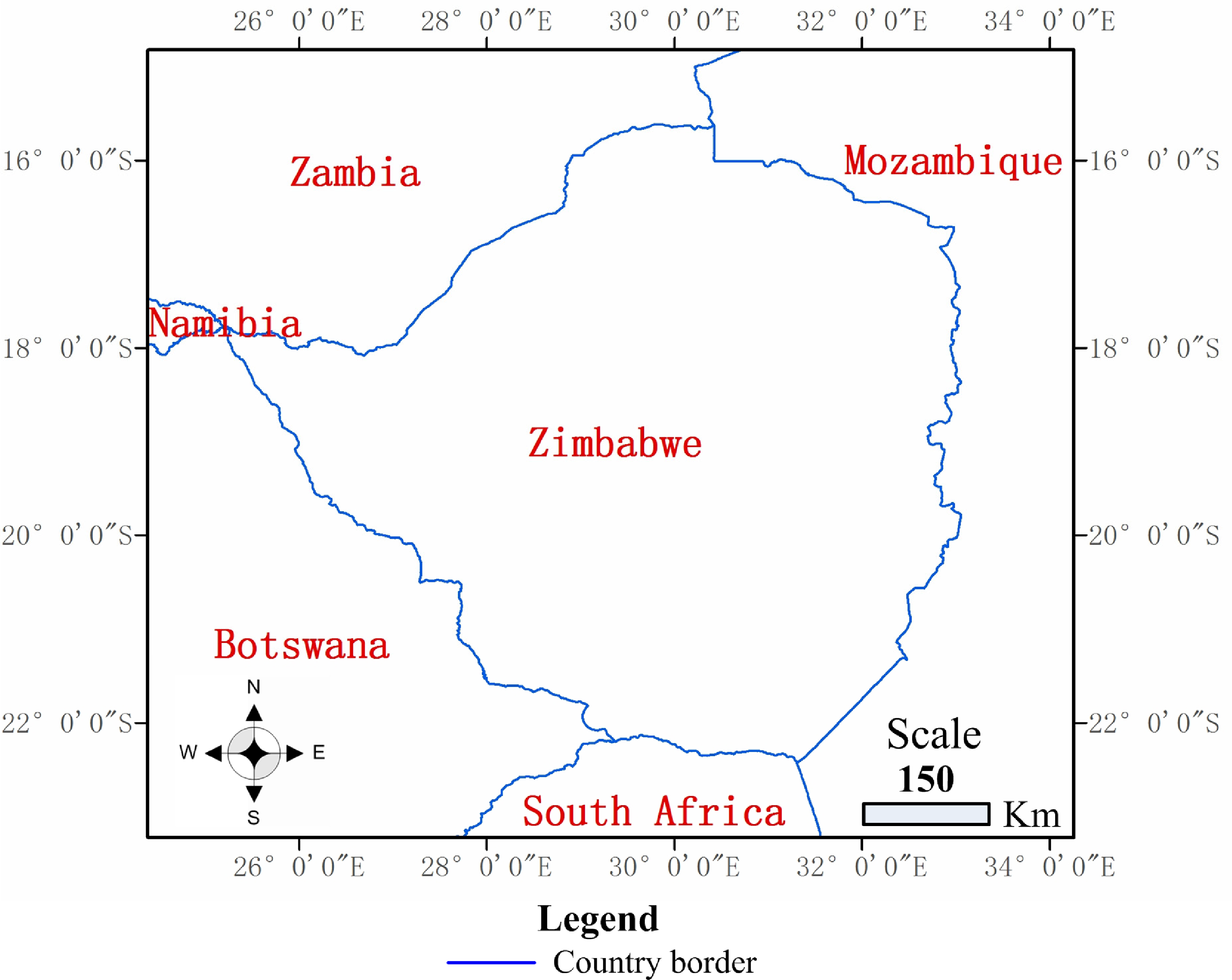
Zimbabwe is a landlocked country in Southern Africa, located between latitudes 15° and 23°S, and longitudes 25° and 34°E. The country is bordered by Zambia, Botswana, Mozambique and South Africa, and meets Namibia at its westernmost point. Zimbabwe’s main industries are agriculture, tourism and mining. There are two categories of agriculture in Zimbabwe, industrialized agriculture, which includes cotton, peanuts, tobacco, coffee and fruits, and subsistence agriculture, which consists of staple crops, such as maize and wheat. These two agricultural types were mainly held by white farmers until the FTLRP was implemented in 2000. The main commercial mining deposits are chromite, coal, asbestos, copper, nickel, gold, platinum and iron ore. Zimbabwe boasts several tourist attractions; the most famous is Victoria Falls, located on the border shared with Zambia. A map showing the location of Zimbabwe is depicted in Figure 1. Zimbabwe is divided into eight provinces: Manicaland, Mashonaland Central, Mashonaland East, Mashonaland West, Masvingo, Matabeleland North, Matabeleland South, Midlands, and two cities with provincial status, Harare (the capital) and Bulawayo.

2.2. Pre-Processing of the DMSP-OLS Nighttime Light Imagery

In this study, we employed the annual stable nighttime light composites from 1992 to 2009. However, these data are not by themselves useful because composites from different years are at different radiometric levels, requiring the data be radiometrically calibrated. Using an inter-calibration model provided a practical solution to the problem. Implementing the model, a composite was viewed as a reference image, and all the other composites were calibrated to the same level of the reference image [30]. The model is a second-order regression written as:

$$y=c_2\hspace{0.17em}{x}^2+c_{1}x+c_0$$

(1)

where x is the original pixel value, y is the calibrated pixel value, and c₀, c₁ and c₂ are coefficients of the polynomial. The coefficients are available in an online document [31]. For those years where data originated from two DMSP-OLS satellites, the two composites were averaged to produce a single composite for that year. Global nighttime composites were transformed from a geographic coordinate system to a Goode Homolosine projection, which is an equal-area projection used for nighttime light analysis [32]. Lastly, the projected composite was resampled at a 1 km resolution. Nighttime light imagery in this study represents the pre-processed data for Zimbabwe. Figure 2 shows the nighttime light imagery in 1992, 2000 and 2008.

3. Detecting Zimbabwe’s Economic Decline Using Nighttime Light Imagery

3.1. National Response of Nighttime Light to Zimbabwe’s Economy

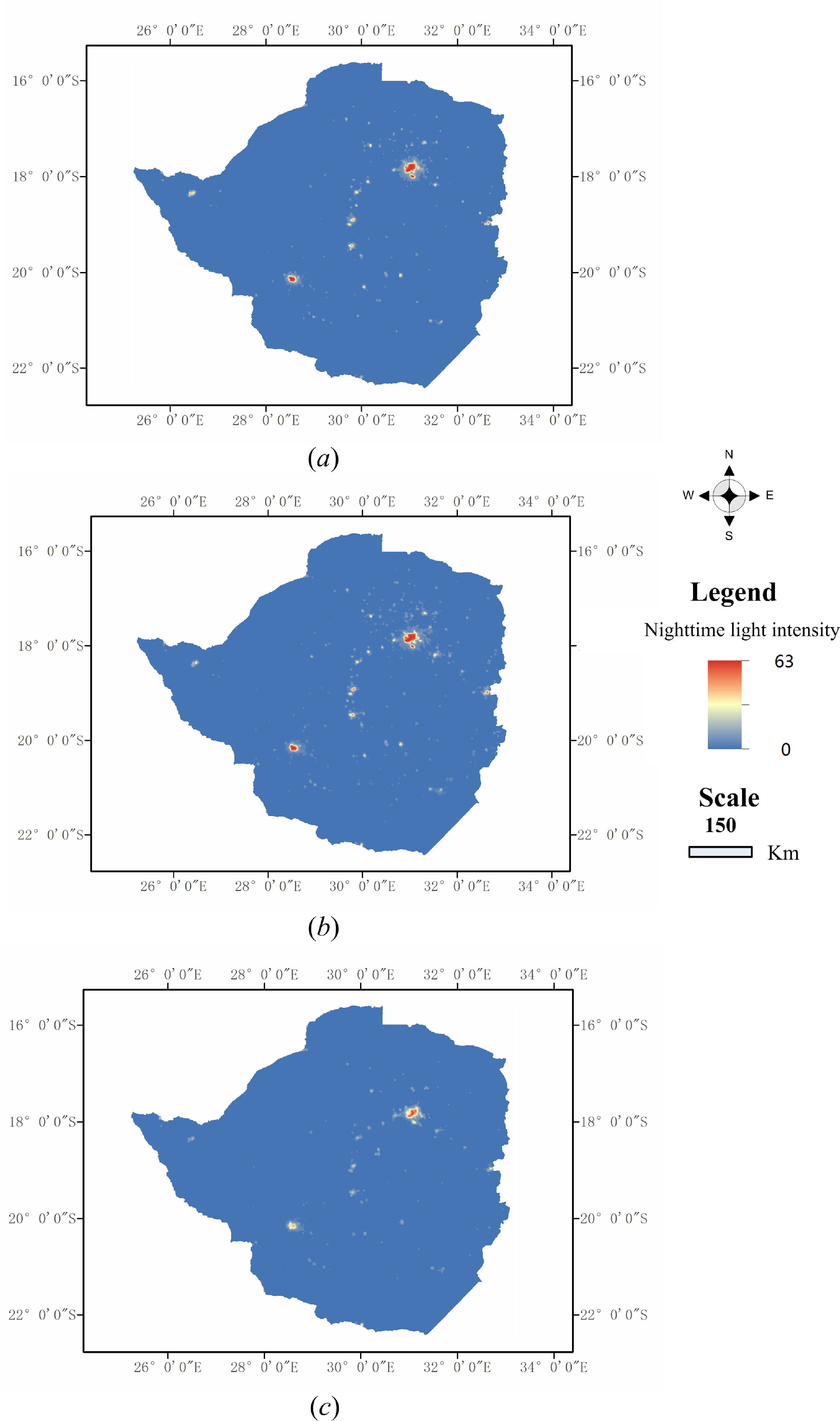
Although a number of studies have investigated Zimbabwe’s economic decline, quantitative analysis is greatly limited, and the degree of the decline in different regions is publicly unknown. DMSP-OLS nighttime light imagery provides continuous social-economic data in spatial and temporal dimensions and can help quantify economic decline in Zimbabwe. Figure 2 shows that the intensity of nighttime light in Zimbabwe was much less in 2008 than in 2000, which may be interpreted as evidence of economic decline. However, this relationship must be proven quantitatively.

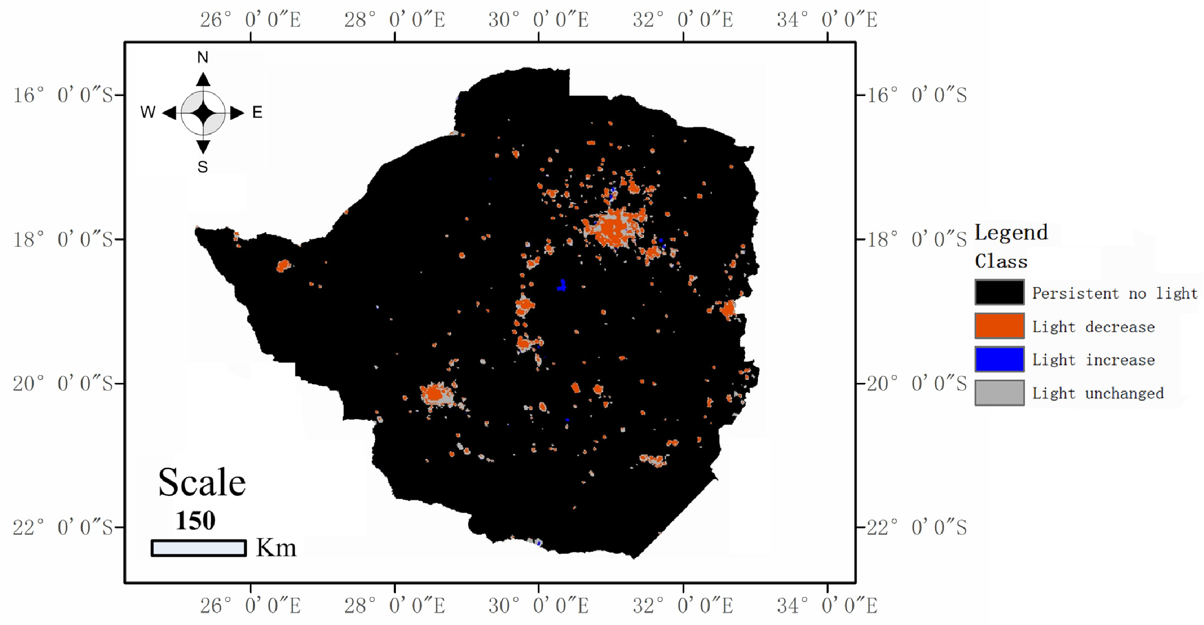
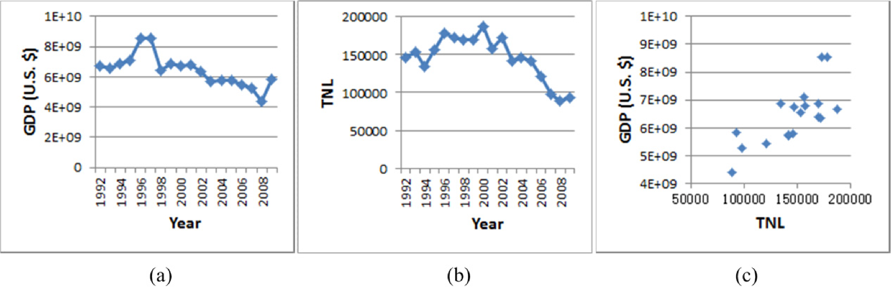
First, data were collected from the World Bank on Zimbabwe’s GDP between 1992 and 2009 [33]. These data are illustrated in Figure 3(a). To find a proxy of GDP on nighttime light imagery, total nighttime light (TNL) was calculated as the sum of all pixel values in a region and then derived for Zimbabwe from 1992 to 2009 as shown in Figure 3(b). The GDP and TNL curves began to decline in 1997 and 2000, respectively. The nadirs of both curves appear in 2008, the year when Zimbabwe’s economy most severely declined. Figure 3(c) shows the scatter diagram of the GDP-TNL relationship. The correlation coefficient is 0.7361. A one-tail Pearson’s significance test was performed on the correlation analysis, and it satisfied a significance level of 0.01. This analysis shows that Zimbabwe’s TNL reflects the GDP data with a strong level of confidence. Admittedly, some fluctuations in GDP do not show a timely response in TNL. For example, GDP decreased starting in 1997, whereas TNL began to decrease in 2000. Despite these inconsistencies, TNL is viewed as an adequate proxy for GDP, not only in this study but in other studies as well [26]. Because the GDP curve shows that 2008 is a nadir of Zimbabwe’s economy, we compared the nighttime light in 2000 and 2008 by generating a difference image. Considering that random factors may influence the comparative results, we defined a threshold of three to judge whether a pixel value changed, as the following formula shows:

$$\mathit{class}=\{\begin{array}{l}\text{Light}\hspace{0.17em}\text{decrease},\mathit{when}\hspace{0.17em}{L}_{2008}-L_{2000}<-3,L_{2008}+L_{2000}>0\hfill \\ \text{Light}\hspace{0.17em}\text{unchanged},\mathit{when}-3\le L_{2008}-L_{2000}\le 3,L_{2008}+L_{2000}>0\hfill \\ \text{Light}\hspace{0.17em}\text{increase},\mathit{when}\hspace{0.17em}3<L_{2008}-L_{2000},L_{2008}+L_{2000}>0\hfill \\ \text{Persistent}\hspace{0.17em}\text{no}\hspace{0.17em}\text{light},\mathit{when}\hspace{0.17em}{L}_{2008}+L_{2000}=0\hfill \end{array}$$

(2)

where L₂₀₀₈ and L₂₀₀₀ denote nighttime light values in 2008 and 2000, respectively. Because a large area of Zimbabwe never produces nighttime light, a persistent no light class is defined in the formula. This is approximate because the light value from 2001 to 2007 is not considered. The difference image is labeled with four classes: persistent no light, light decrease, light increase and light unchanged. Figure 4 shows the spatial distribution of the four classes across Zimbabwe, where there is 440,546 km² of persistent no light, 10,876 km² of light decrease, 415 km² of light increase and 9726 km² of light unchanged. The map reveals a decrease in more than half of the lit area from 2000 to 2008, while a small number of areas emitted more light and the light in some areas was unchanged.

3.2. Classification of the Regions

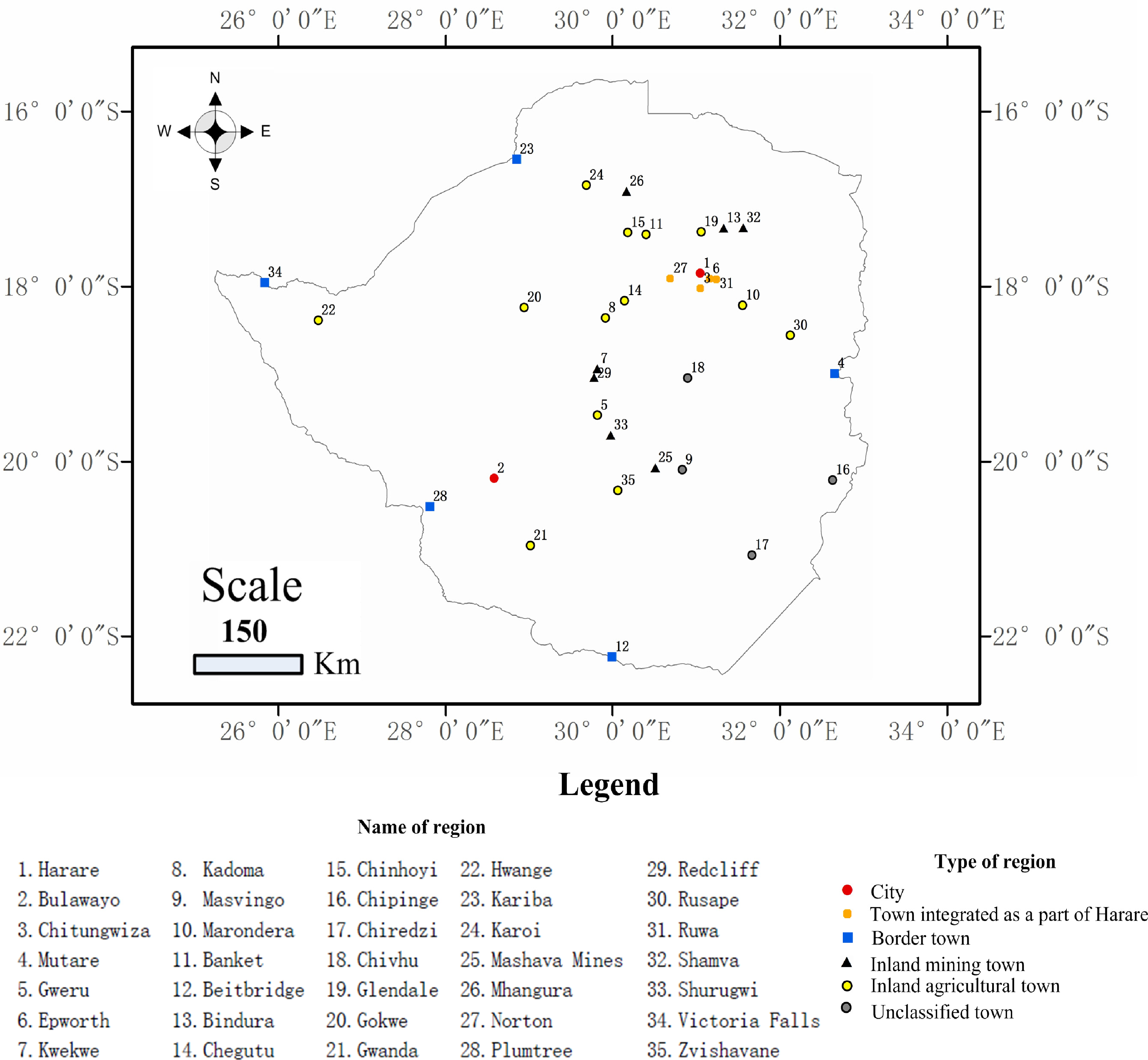
There is a strong correlation between nighttime light and GDP in Zimbabwe from 1992 to 2009. Because nighttime light imagery has been successfully employed as a proxy to measure global and regional economic changes, we used nighttime light imagery to measure the severity of economic decline in different regions and economic sectors of Zimbabwe. For our analysis, we selected 35 regions (

Table 1. List of the 35 regions and their types.

Type of Regions	Regions
City	Harare (including Norton, Epworth, Ruwa and Chitungwiz) and Bulawayo
Border town	Kariba, Victoria Falls, Plumtree, Beitbridge and Mutare
Inland mining town	Mashava Mines, Shamva, Bindura, Kwekwe, Shurugwi, Redcliff and Mhangura
Inland agricultural town	Banket, Karoi, Marondera, Chegutu, Chinhoyi, Rusape, Gokwe, Gweru, Hwange, Kadoma, Gwanda, Glendale and Zvishavane
Unclassified	Chipinge, Masvingo, Chiredzi and Chivhu

and Figure 5), which included all major cities and towns defined to be major human settlements in Zimbabwe [34]. Using Google Earth, we located the center of each region and mapped each as a point. Four regions, Norton, Epworth, Ruwa and Chitungwiz, were integrated into Harare because they were considered as satellite towns of Harare. The 31 remaining regions were then classified by type based on their predominant economic sector and geography.

A. Cities and border towns

Harare and Bulawayo were classified as cities because of their large populations and important economic role in Zimbabwe (

Table 2. Total nighttime light of the regions in Zimbabwe in 2000 (TNL₂₀₀₀) and 2008 (TNL₂₀₀₈), and population in 2002 (POP₂₀₀₂).

Region	Region Type	POP2002	TNL2000	TNL2008	Change (%)	Change Type
Mashava Mines	Inland mining town	12,315	1,024	114	−89	Severe
Shamva	Inland mining town	9,437	778	161	−79	Severe
Banket	Inland agricultural town	9,845	421	95	−77	Severe
Karoi	Inland agricultural town	22,383	691	184	−73	Severe
Bindura	Inland mining town	33,637	2,060	632	−69	Severe
Mhangura	Inland mining town	5,747	230	79	−66	Severe
Chegutu	Inland agricultural town	43,424	1,463	503	−66	Severe
Gokwe	Inland agricultural town	17,703	519	185	−64	Severe
Marondera	Inland agricultural town	51,847	2,784	1,011	−64	Severe
Kwekwe	Inland mining town	93,608	4,178	1,532	−63	Severe
Mutare	Border town	170,466	4,306	1,630	−62	Severe
Chinhoyi	Inland agricultural town	48,912	1,554	610	−61	Severe
Rusape	Inland agricultural town	22,741	727	296	−59	Severe
Hwange	Inland agricultural town	34,950	2,779	1244	−55	Severe
Redcliff	Inland mining town	32,417	1,528	687	−55	Severe
Zvishavane	Inland agricultural town	35,128	1,069	488	−54	Severe
Gweru	Inland agricultural town	140,806	4,038	2,020	−50	Medium
Kadoma	Inland agricultural town	76,351	2,075	1,104	−47	Medium
Gwanda	Inland agricultural town	13,184	447	239	−47	Medium
Shurugwi	Inland mining town	16,863	705	400	−43	Medium
Bulawayo	City	676,650	19,399	11,074	−43	Medium
Harare	City	1,955,219	54,250	33,189	−39	Medium
Victoria Falls	Border town	31,519	1,058	679	−36	Medium
Plumtree	Border town	9,923	382	268	−30	Medium
Kariba	Border town	22,726	737	582	−21	Slight
Glendale	Inland agricultural town	9798	690	622	−10	Slight
Beitbridge	Border town	22,136	1,033	1,173	14	Increase

). Kariba, Victoria Falls, Plumtree, Beitbridge and Mutare were separated and defined as border towns because international trade may play an important role in these towns. The remaining regions were classified as inland towns, and then further grouped by economic sectors.

B. Inland mining towns and agricultural towns

Zimbabwe’s major economic sectors are agriculture, manufacturing, service and mining. For the inland towns, we concentrated only on the agriculture and mining sectors because they are the economic pillars upon which the other sectors are based. For example, major manufacturing products are mainly derived from domestic mining and agricultural activities.

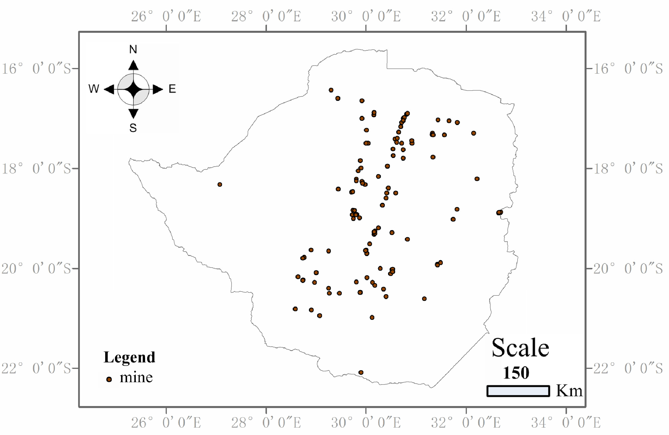
All inland towns were classified into two sector types, agricultural and mining. We defined mining towns to be those towns located closest to mines. A global mine dataset with accurate positions was acquired from the United States Geological Survey to achieve this purpose [35]. Then, those mines operating in 2000 were selected as shown in Figure 6. For each operating mine, a buffer zone with a 3 km radius was delineated, and a nationwide mining area was mapped. We found that seven towns (Mashava Mines, Shamva, Bindura, Kwekwe, Shurugwi, Redcliff and Mhangura) fell within mining areas. These towns are classified as mining towns.

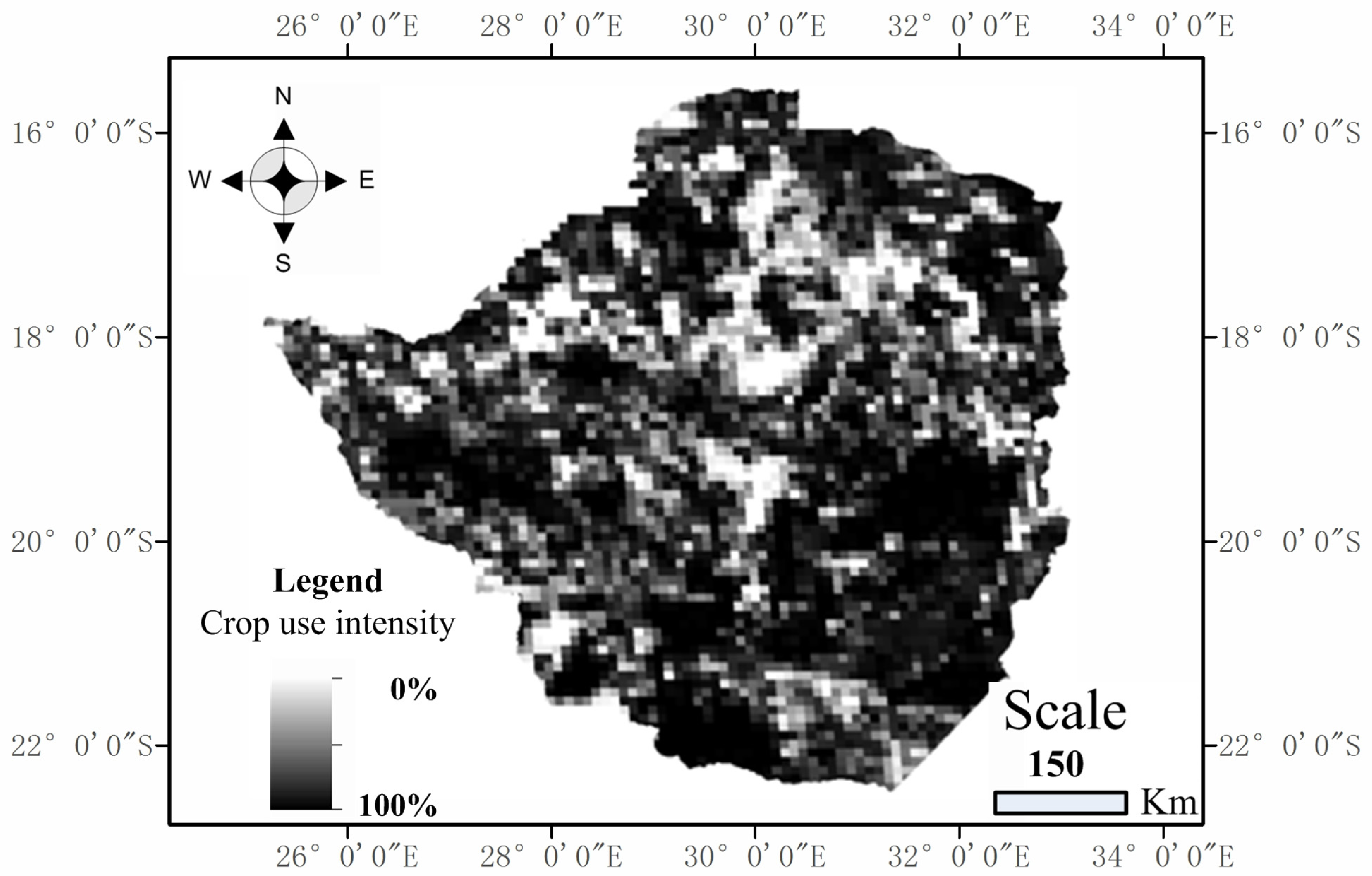
After identifying cities, borders and mining towns, the remaining regions close to major croplands were classified as agricultural towns. Using a national crop use intensity map (Figure 7) [36], we classified those areas with crop use intensity greater than 30% to be well-developed agricultural areas and delineated a 10 km buffer zone that comprised the adjacent area. Regions falling within the buffer zone were classified as agricultural towns because they depend on agriculture heavily. Twelve inland towns (Banket, Marondera, Chegutu, Chinhoyi, Rusape, Gokwe, Gweru, Hwange, Kadoma, Gwanda, Glendale and Zvishavane) were classified as inland agricultural towns.

C. Unclassified towns

After the four types of regions were defined, four inland towns, Chipinge, Masvingo, Chiredzi and Chivhu, remained unclassified. These towns were not analyzed in this study.

D. Delineating the regions

Twenty-seven regions were classified into the four region types as illustrated in Figure 5. Buffer zones were created for each region point to delineate the scope of the region. For each town selected, a buffer zone with a 10 km radius delineated the town area because, for most towns, 10 km is long enough to encompass all human settlements. For each city, a buffer zone with a 40 km radius delineated the urban area as this distance is large enough to comprise most of the urban and suburban lighting captured in the nighttime light imagery. The buffer zones of Redcliff and Kwekwe were found to overlap, so an equidistant line was drawn between the towns to modify the two buffer zones and make them independent from each other. The buffer areas of border towns beyond the national boundary were discarded. Thus, buffer zones for all regions were derived for nighttime light analysis.

3.3. Nighttime Light Change in Different Types of Regions

To estimate the severity of economic decline, we compared the nighttime light images from 2000, when the FTLRP was initiated, to images in 2008. The amount of nighttime light for each region was calculated for both 2000 and 2008 (Table 2). A change rate index, used to measure light change, was calculated using the following equation:

$$r=\frac{L_{2008}-L_{2000}}{L_{2000}}$$

(3)

where r denotes the relative change of nighttime light from 2000 to 2008, and L₂₀₀₀ and L₂₀₀₈ represent total nighttime light in 2000 and 2008, respectively. The TNL of all 27 regions in 2000 was 110,925, whereas the TNL of Zimbabwe in 2000 was 150,892. Therefore, these regions emitted 74% of Zimbabwe’s nighttime light in 2000 and are representative for analyzing Zimbabwe’s economy. Generally, nighttime light in most regions experienced a sharp decrease, but Beitbridge was an exception.

To evaluate nighttime light variation in different types of regions, the overall change rate was calculated, which is defined as the change rate of nighttime light in each type of region. To compare light change in different region types, we classified light change into four distinct levels: severe decrease (r < −50%), moderate decrease (−50% < r < −25%), slight decrease (−25% < r < 0) and increase (0 < r).

Table 3. The nighttime light change in different types of regions in Zimbabwe.

Region Type	Per cent of Different Change Levels of Nighttime Light (%)				Overall Change Rate (%)
	Severe Decrease	Moderate Decrease	Slight Decrease	Increase
Inland mining town	85.71	14.29	0	0	−65.68
Inland agricultural town	69.23	23.08	7.69	0	−55.34
City	0	100	0	0	−39.90
Border town	20	40	20	20	−42.36

shows the per cent of different light change in the four region types. For example, of the seven inland mining towns, six towns experienced severe nighttime light decrease, as listed in Table 2. Therefore, 85.71% of inland mining towns exhibited nighttime light decrease, as shown in Table 3.

According to Table 3, inland mining towns were most severely impacted by the economic decline; 85.71% experienced severe light decrease and 14.29% experienced moderate light decrease. Although inland agricultural towns were also severely impacted by the economic decline, they were not impacted as severely as inland mining towns; 69.23%, 23.08% and 7.69% had severe, moderate and slight decreases, respectively. The overall nighttime light change rates of inland mining (−65.68%) and agricultural towns (−55.34%) show that they too were severely impacted by economic decline. The situation in the cities was better. Both cities exhibited only a moderate decrease of nighttime light, and the overall change rate was −39.90%. The situation in the border towns was complex. Of the five border towns, 20% exhibited a severe decrease, 40% exhibited a moderate decrease, 20% exhibited a slight decrease and 20% exhibited an increase. Despite the complexity, the overall change rate of nighttime light in the border towns was relatively small (−42.36%).

A. Nighttime light in the inland mining towns

We found that nighttime light in Zimbabwe’s inland mining towns decreased the most of the four region types, leading us to infer that the mining sector severely declined. In fact, Zimbabwe’s mining industry nearly collapsed, along with agriculture and other economic sectors.

Table 4. The mineral output of Zimbabwe in 2001 and 2008 [37].

Mineral	Output		Change (%)	Mineral	Output		Change (%)
	2001	2008			2001	2008
Asbestos (ton)	136,327	11,489	−92	Lithium minerals (ton)	36,103	0	−100
Black Granite (ton)	385,532	0	−100	Low Carbon Ferrochrome (ton)	6,307	0	−100
Chrome (ton)	780,150	442,584	−43	Magnesite (ton)	2,439	2,548	4
Coal (ton)	4,064,497	1,701,599	−58	Nickel (ton)	8,145	6,354	−22
Cobalt (ton)	95	28	−71	Palladium (kg)	371	4,274	1052
Copper (ton)	2,057	2,826	37	Phosphate (ton)	878,80	21,439	−76
Feldspar (ton)	1,055	0	−100	Platinum (kg)	519	5,495	959
Ferrosilicon (ton)	16,848	1611	−90	Quartz rough (ton)	28,162	0	−100
Fireclay (ton)	3404	0	−100	Rhodium (kg)	42	443	955
Gold (kg)	18,050	0	−100	Silica (ton)	14,544	0	−100
Graphite (ton)	11,837	5,134	−57	Silver (kg)	3,344	0	−100
High Carbon Ferrochrome (ton)	243,534	145,430	−40	Slate (ton)	435	0	−100
Iron Ore (ton)	360,862	2,919	−99	Talc (ton)	1,272	0	−100
Iron Pyrite (ton)	98,037	30,308	−69	Tantalite (ton)	30	0	−100
Kyanite (ton)	9,682	0	−100	Vermiculite (ton)	11,632	16,123	39
Limestone (ton)	3,798,956	0	−100

shows the production of Zimbabwe’s main minerals in 2001 and 2008 (data from 2001 is used in place of data from 2000). Mining of most minerals decreased significantly, with the exception of Copper, Palladium, Platinum and Rhodium. In 2008, mining of fourteen minerals, such as Black Granite, Feldspar and Fireclay, completely stopped, and production of some pillar minerals, such as asbestos, gold, coal and nickel, declined sharply. Thus, nighttime light in mining towns decreased severely, as shown in this analysis. It is worth noting that during this period of economic decline, Zimbabwe increasingly exploited Platinum group metals (e.g., Palladium, Platinum and Rhodium) to generate export earnings. Nevertheless, increased production of these minerals could not compensate for the large decrease in light observed in the mining towns, as shown in Table 4. The analysis shows that observable nighttime light reflects the changes in Zimbabwe’s mining sector.

B. Nighttime light in the inland agricultural towns

Agriculture is the backbone of Zimbabwe’s economy, although it only constitutes approximately 10% of Zimbabwe’s GDP. The production of two major food crops and two major cash crops in 2000 and 2008 is listed in

Table 5. The production of maize, wheat, cotton and tobacco in Zimbabwe in 2000 and 2008 [38].

Food Crop	Production		Change (%)	Cash Crop	Production		Change (%)
	2000	2008			2000	2008
Maize (1,000 t)	1620	471	−71	Cotton (1,000 t)	337	247	−27
Wheat (1,000 t)	230	31	−87	Tobacco (1,000 t)	202	64	−68

. Production of all four crops fell significantly between 2000 and 2008. Specifically, the two food crops, maize and wheat, which are crucial staples of the Zimbabwean people, decreased by −71% and −87%, respectively. Cotton production fared relatively better, decreasing by −27%. Generally, agricultural production was severely impacted by the FTLRP, which is consistent with the decrease in nighttime light in the inland agricultural towns. However, agricultural decline was not as severe as that of the mining industry, where production of some minerals stopped or nearly stopped, while all crops continue to be produced. Overall nighttime light change rates support this finding. Light decreased by −65.68% in inland mining towns and −55.34% in inland agricultural towns.

C. Nighttime light in the cities

Harare and Bulawayo are the only two cities in Zimbabwe. Economic data for these two cities are publicly unavailable. The major economic sectors in these two cities are services and manufacturing. The overall nighttime light change rate of the two cities was −39.90%, which is much lower than the rate of inland agricultural and mining towns. Thus, we can infer that the economy in Zimbabwe’s cities during the economic decline was better than in mining and agriculture towns because the service industry was not impacted as severely. Furthermore, streetlights, as part of urban infrastructure, are important lighting sources in cities, and even during harsh economic times, municipalities will maintain these sources.

D. Nighttime light in the border towns

Border town economies rely heavily on international trade; therefore, international trade should be an important component of the economy in these regions. Although some goods may be transported by plane, land ports are the primary route for international trade in Zimbabwe. We based these assertions on Zimbabwe’s international trade volume in 2000 and 2008, as obtained from the World Bank and shown in

Table 6. The total volume of international trade of Zimbabwe in 2000 and 2008 [40].

	Import Value (million $)	Export Value (million $)	Total Export-Import Volume
2000	240.22	255.29	495.51
2008	300.80	183.28	484.08
Change rate	25.22%	−28.21%	−2.31%

. Although Zimbabwe’s economy declined severely between 2000 and 2008, international trade did not perform as poorly. Imports increased by 25.22%, and exports decreased by −28.21%. Total export-import volume decreased by only −2.31% compared to a −34.00% decrease in GDP during the same period. In addition to official data, underground trade is also rampant in some border towns, where some unemployed earn a living smuggling goods [39].

Among the five border towns, only Mutare experienced a severe decrease in nighttime light. The total change rate was −42.36%, which was less than that of the inland mining and agricultural towns. Mutare is located along the Mozambique border, where Zimbabwe’s international trade is very limited, whereas the economic volume of Mutare is large given that its TNL was greater than 4000 in 2000. Therefore, the impact of international trade on Zimbabwe’s economy is very limited. This may explain why nighttime light severely decreased in this border town.

It is interesting to note that nighttime light in Beitbridge, located on the Zimbabwe-South Africa border, increased between 2000 and 2008. This increase may be a result of a growing border trade of legal and illegal goods [39]. South Africa is Zimbabwe’s largest trade partner, and a large number of goods destined for foreign countries (e.g., the United Kingdom, United States and China) are transported through Beitbridge. Victoria Falls, Plumtree and Kariba are adjacent to Zambia, Botswana and Zambia, respectively. The total economic volume of these three towns is not so large that a thriving international trade would significantly impact them. Additionally, because Kariba is a major hydroelectric centre, and Victoria Falls is the most famous tourist resort in Zimbabwe, we infer that hydroelectric and tourism industries were not as severely impacted as agriculture and mining industries during the economic decline.

3.4. Accuracy Estimation

We have revealed that different regions and economic sectors in Zimbabwe have different economic decline by use of the nighttime light data analysis, assuming that the nigttime light change is caused by the economic fluctuation, which has been proven previously [14]. It is also necessary to quantitatively estimation how accurate the nighttime light responds to the economic decline in Zimbabwe. As the regional economic data of Zimbabwe is unavailable, this estimation is hard to carry out with the real regional data. As an alternative, we use the national GDP and TNL data of Zimbabwe to simulate the evaluation data, and then evaluate the relationship between GDP change and TNL change.

As stated in Section 3.1, a time series GDP and TNL data of Zimbabwe between 1992 and 2009 has been derived, which is used as data for accuracy estimation here. For the 18 years, there are GDP and TNL data for each year. We randomly select any two years as sampling years, and sample i is denoted as {t_i1, g_i1, t_i2, g_i2} where t_i1 and g_i1 represent the TNL and GDP data respectively for the first selected year of sample i, and t_i2 and g_i2 represent the TNL and GDP data respectively for the second selected year of sample i. For sample i, we can calculate its TNL change rate as

$$r_{\mathit{TNL}}^{(i)}=\frac{t_{i2}-t_{i1}}{t_{i1}}$$

(4)

and calculate the GDP change rate as

$$r_{\mathit{GDP}}^{(i)}=\frac{g_{i2}-g_{i1}}{g_{i1}}$$

(5)

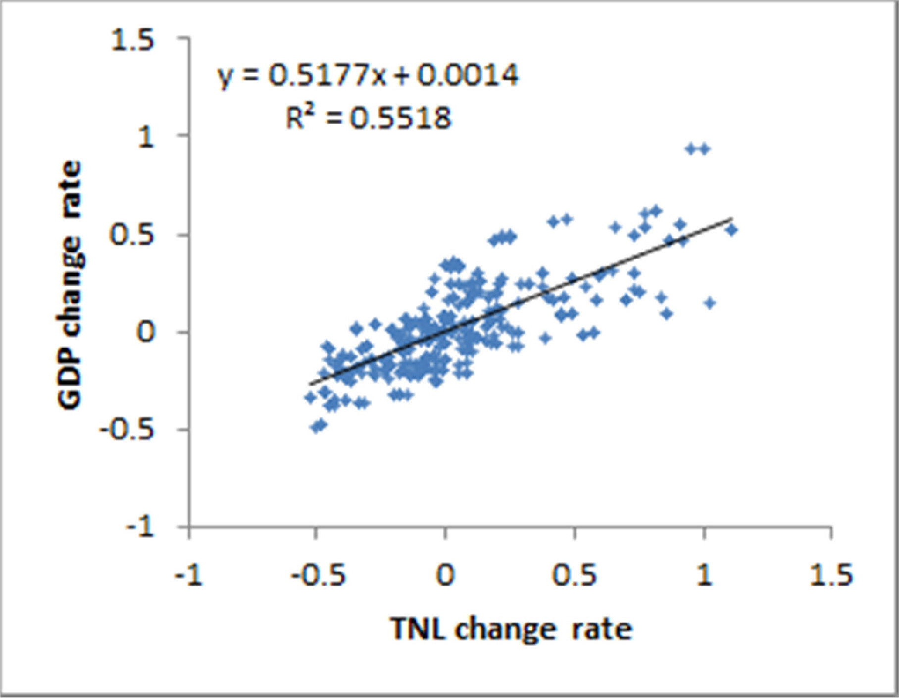
Consequently, for each sample i, we get its TNL and GDP change rates as $r_{\mathit{TNL}}^{(i)}$ and $r_{\mathit{GDP}}^{(i)}$ respectively. Totally, we have sampled for 500 times with the same strategy, and then we get 500 samples and their associated TNL and GDP change rates. As illustrated in Figure 8, a scatter diagram and a linear regression model are derived from the samples to show the relationship between TNL change rate and GDP change rate for Zimbabwe.

We found that the R² of this linear regression is 0.5518, showing that the TNL change rate has good correlation with GDP change rate in Zimbabwe. Then, we input the TNL change rate from the samples into the regression model to get the estimated GDP data. For each estimated GDP value, we assess its error with the following formula:

$$e_{\mathit{GDP}}^{(i)}=\left|{\widehat{r}}_{\mathit{GDP}}^{(i)}-r_{\mathit{GDP}}^{(i)}\right|$$

(6)

where ${\widehat{r}}_{\mathit{GDP}}^{(i)}$ denotes the estimated GDP change rate from the TNL change rate in sample i, $r_{\mathit{GDP}}^{(i)}$ denotes the real GDP change rate in sample i, and $e_{\mathit{GDP}}^{(i)}$ denotes the estimation error of GDP change rate from TNL change rate in sample i. Then each sample is associated with an estimation error, and we got 500 numbers of estimation errors shown in

Table 7. The distribution of the estimation error of GDP change rate from TNL change rate, where e denotes the error.

Range	0 ≤e< 10%	10% ≤e< 20%	20% ≤e< 30%	30% ≤e< 40%	40% ≤e≤ 50%
Number	260	157	54	25	4
Ratio	52%	31.4%	10.8%	5%	0.8%

.

From Table 7, we found that 52% of the estimation errors are smaller than 10%, and 31.4% of the estimation errors are larger than 10% but less than 20%, therefore there are totally 83.4% of the estimation errors smaller than 20%. Although some errors have large values, they only constitute a small part (e.g., 0.8% of the errors are larger than or equal to 40%). Besides, we averaged all the estimation errors, and then we found that the overall estimation error is 11.35%. In other words, when estimating Zimbabwe’s GDP change rate by use of the TNL change rate from any two years, the expected error should be 11.35%. These findings show that the accuracy of estimated GDP change rate is satisfactory considering that there are a number of pair of years with large temporal gap like ten years or more.

In summary, from the above accuracy analysis, the nighttime light change rates in different regions of Zimbabwe can generally reflect the economic decline, showing that the discovered economic decline pattern is reliable.

4. Discussion

A number of studies have analyzed Zimbabwe’s economic decline from different economic sectors [2–8], while very few of them have provided spatial information, so that the picture of the economic decline is unclear to international community. In fact, the spatial information of the economic decline can help to understand the effect of FTLRP on different regions of Zimbabwe. For example, do different land redistribution strategies during FTLRP have different impacts on the regional economy? Unfortunately, obtaining the spatial information at national scale needs a lot of field work, which is not easily undertaken by the academic community.

Remote sensing technique, which can provide continuously spatial and temporal information, has played an important role in natural resources studies of Zimbabwe, such as agriculture [41,42], forestry [43] and climate [44]. Although remote sensing of natural resources may help to understand the socio-economic aspects of the country, it is not an efficient way because the economic decline should have complicated interactions with the natural resources. Therefore, remote sensing of human activities in Zimbabwe can provide a more effective mirror for the economic decline. A few studies of Zimbabwe on land cover change mapping [45] and human settlement detection [46] seem to have stronger link to the socioeconomic aspects. However, these works made use of medium or high resolution remote sensing imagery, which is too costly when applied in national scale.

Among various types of remote sensing images, nighttime light images provide a unique human perspective on the earth surfaces, because the images directly reflect regional economy and population density. A number of studies have employed the nighttime light imagery in rapidly growing countries like China [12,26] and India [23] and developed countries like European states [10]. Based on these successful experiences, we employed the DMSP-OLS nighttime light imagery as the first attempt to detect Zimbabwe’s economic decline. Using the imagery at both national and regional scales, we found that it reflects the economic decline that transpired during Zimbabwe’s FTLRP. More than half of the previously lit areas in Zimbabwe experienced a decrease in nighttime light. Because TNL has a strong correlation with Zimbabwe’s GDP, nighttime light is an adequate indicator for Zimbabwe’s economy. As the various economic sectors performed differently during the economic decline, the associated regions have different nighttime light decline.

5. Conclusion

Once a prosperous Southern African nation, Zimbabwe has suffered severe economic decline during 2000–2008. Although the process and aftermath of Fast Track Land Reform Program (FTLRP) were controversial, and Zimbabwe’s economic decline is widely known by the international community, the pattern of economic decline in Zimbabwe is not very clear. To clarify the issue, we used Defense Meteorological Satellite Program’s Operational Linescan System (DMSP-OLS) nighttime light imagery to investigate the spatial pattern of economic decline because nighttime light is considered to be an indicator reflecting global and regional economic change.

We found that total nighttime light (TNL) from 1992 to 2009 reflected the decline in Zimbabwe’s gross domestic product (GDP) with correlation coefficient as 0.7361, which suggests that the nighttime light images are valuable for reflecting economic trends in Zimbabwe. More importantly, by comparing nighttime light images in 2000 and 2008, the nighttime light change in four regional types (generally, −65.68% for the inland mining towns, −55.34% for the inland agricultural towns, −39.90% for the cities and −42.36% for the border towns) approximately reflects the economic decline in different economic sectors. We conclude that mining and agricultural sectors were severely impacted, whereas the service industry in cities and international trade in border towns were impacted less severely. Our analysis on the relationship between nighttime light and economic decline is primary and semi-quantitative because precise economic data are publicly unavailable. Therefore, it is hard to rigorously validate economic decline based solely on nighttime light imagery, although remote sensing does have its advantages when economic data are lacking.

In contrast to previous studies that focused on nighttime light related to regional and global economic growth [14,26], this regional case study utilizes nighttime light images to investigate economic decline. It seems natural that nighttime light reflects economic decline because economic growth leads an increase in nighttime light. However, this relationship should be proven through case studies like this one. If nighttime light images are captured at higher spatial and temporal resolutions, more details on economic variation will be revealed, and the recent emerging of the Suomi National Polar-orbiting Partnership (Suomi NPP) satellite provides a better nighttime light source with higher spatial resolution and radiometric quality. Our future work can focus on the application of the Suomi NPP nighttime light imagery in detecting the socio-economic fluctuation in some countries where the survey data are publicly unavailable.

References

- Cliffe, L.; Alexander, J.; Cousins, B.; Gaidzanwa, R. An overview of fast track land reform in Zimbabwe: Editorial introduction. J. Peasant Stud 2011, 38, 907–938. [Google Scholar]
- Mzumara, M. Was Zimbabwe competitive in international trade 2000–2009? Int. J. Econ. Bus. Res 2011, 2, 195–216. [Google Scholar]
- Masuka, G. Contests and struggle: Cotton farmers and COTTCO in Rushinga district, Zimbabwe, 1999–2006. Geoforum 2012, 43, 573–584. [Google Scholar]
- Obi, A.; Chisango, F.F. Performance of smallholder agriculture under limited mechanization and the fast track land reform program in Zimbabwe. Int. Food Agribus. Manag. Rev 2011, 14, 85–104. [Google Scholar]
- Baudron, F.; Tittonell, P.; Corbeels, M.; Letourmy, P.; Giller, K.E. Comparative performance of conservation agriculture and current smallholder farming practices in semi-arid Zimbabwe. Field Crops Res 2012, 132, 117–128. [Google Scholar]
- Nyota, S.; Sibanda, F. Digging for diamonds, wielding new words: A linguistic perspective on Zimbabwe’s “Blood Diamonds”. J. South. Afr. Stud 2012, 38, 129–144. [Google Scholar]
- Chiripanhura, B.M. Sneaking up and stumbling back: Textiles sector performance under crisis conditions in Zimbabwe. J. Int. Dev 2010, 22, 153–175. [Google Scholar]
- Mhiripiri, N.A. The production of stardom and the survival dynamics of the Zimbabwean music industry in the post-2000 crisis period. J. Afr. Media Stud 2010, 2, 209–223. [Google Scholar]
- Famine Early Warning Systems Network. Available online: http://www.fews.net (accessed on 5 September 2013).
- Doll, C.N.H.; Muller, J.P.; Morley, J.G. Mapping regional economic activity from night-time light satellite imagery. Ecol. Econ 2006, 57, 75–92. [Google Scholar]
- Elvidge, C.D.; Sutton, P.C.; Ghosh, T.; Tuttle, B.T.; Baugh, K.E.; Bhaduri, B.; Bright, E. A global poverty map derived from satellite data. Comp. Geosci 2009, 35, 1652–1660. [Google Scholar]
- Li, X.; Xu, H.; Chen, X.; Li, C. Potential of NPP-VIIRS nighttime light imagery for modeling the regional economy of China. Remote Sens 2013, 5, 3057–3081. [Google Scholar]
- Chen, X.; Nordhaus, W.D. Using luminosity data as a proxy for economic statistics. Proc. Natl. Acad. Sci. USA 2011, 108, 8589–8594. [Google Scholar]
- Henderson, V.; Storeygard, A.; Weil, D.N. A bright idea for measuring economic growth. Am. Econ. Rev 2011, 101, 194–199. [Google Scholar]
- Ghosh, T.; Anderson, S.; Powell, R.L.; Sutton, P.C.; Elvidge, C.D. Estimation of Mexico’s informal economy and remittances using nighttime imagery. Remote Sens 2009, 1, 418–444. [Google Scholar]
- Zhuo, L.; Ichinose, T.; Zheng, J.; Chen, J.; Shi, P.J.; Li, X. Modelling the population density of China at the pixel level based on DMSP/OLS non-radiance-calibrated night-time light images. Int. J. Remote Sens 2009, 30, 1003–1018. [Google Scholar]
- Bharti, N.; Tatem, A.J.; Ferrari, M.J.; Grais, R.F.; Djibo, A.; Grenfell, B.T. Explaining seasonal fluctuations of measles in Niger using nighttime lights imagery. Science 2011, 334, 1424–1427. [Google Scholar]
- Zhang, Q.L.; Seto, K.C. Mapping urbanization dynamics at regional and global scales using multi-temporal DMSP/OLS nighttime light data. Remote Sens. Environ 2011, 115, 2320–2329. [Google Scholar]
- Small, C.; Pozzi, F.; Elvidge, C.D. Spatial analysis of global urban extent from DMSP-OLS night lights. Remote Sens. Environ 2005, 96, 277–291. [Google Scholar]
- Zhang, Q.; Seto, K. Can night-time light data identify typologies of urbanization? A global assessment of successes and failures. Remote Sens 2013, 5, 3476–3494. [Google Scholar]
- Prasad, V.K.; Kant, Y.; Gupta, P.K.; Elvidge, C.; Badarinath, K. Biomass burning and related trace gas emissions from tropical dry deciduous forests of India: A study using DMSP-OLS data and ground-based measurements. Int. J. Remote Sens 2002, 23, 2837–2851. [Google Scholar]
- Waluda, C.; Yamashirob, C.; Elvidge, C.; Hobson, V.; Rodhouse, P. Quantifying light-fishing for Dosidicus gigas in the eastern Pacific using satellite remote sensing. Remote Sens. Environ 2004, 91, 129–133. [Google Scholar]
- Chand, T.R.K.; Badarinath, K.V.S.; Elvidge, C.D.; Tuttle, B.T. Spatial characterization of electrical power consumption patterns over India using temporal DMSP-OLS night-time satellite data. Int. J. Remote Sens 2009, 30, 647–661. [Google Scholar]
- Agnew, J.; Gillespie, T.W.; Gonzalez, J.; Min, B. Baghdad nights: Evaluating the US military “surge” using nighttime light signatures. Environ. Plan. A 2008, 40, 2285–2295. [Google Scholar]
- Aubrecht, C.; Elvidge, C.; Longcore, T.; Rich, C.; Safran, J.; Strong, A.; Eakin, C.; Baugh, K.; Tuttle, B.; Howard, A. A global inventory of coral reef stressors based on satellite observed nighttime lights. Geocarto Int 2008, 23, 467–479. [Google Scholar]
- Ma, T.; Zhou, C.; Pei, T.; Haynie, S.; Fan, J. Quantitative estimation of urbanization dynamics using time series of DMSP/OLS nighttime light data: A comparative case study from China’s cities. Remote Sens. Environ 2012, 124, 99–107. [Google Scholar]
- Liu, Z.F.; He, C.Y.; Zhang, Q.F.; Huang, Q.X.; Yang, Y. Extracting the dynamics of urban expansion in China using DMSP-OLS nighttime light data from 1992 to 2008. Landsc. Urban Plan 2012, 106, 62–72. [Google Scholar]
- He, C.Y.; Ma, Q.; Li, T.; Yang, Y.; Liu, Z.F. Spatiotemporal dynamics of electric power consumption in Chinese Mainland from 1995 to 2008 modeled using DMSP/OLS stable nighttime lights data. J. Geogr. Sci 2012, 22, 125–136. [Google Scholar]
- Zhao, N.Z.; Samson, E.L. Estimation of virtual water contained in international trade products using nighttime imagery. Int. J. Appl. Earth Observ. Geoinf 2012, 18, 243–250. [Google Scholar]
- Elvidge, C.D.; Ziskin, D.; Baugh, K.E.; Tuttle, B.T.; Ghosh, T.; Pack, D.W.; Erwin, E.H.; Zhizhin, M. A fifteen year record of global natural gas flaring derived from satellite data. Energies 2009, 2, 595–622. [Google Scholar]
- Elvidge, C.D.; Sutton, P.C.; Baugh, K.E.; Ziskin, D.; Ghosh, T.; Anderson, S. National trends in satellite observed lighting: 1992–2012. Available online: http://ngdc.noaa.gov/eog/dmsp/download_national_trend.html (accessed on 5 September 2013).
- Elvidge, C.D.; Baugh, K.E.; Kihn, E.A.; Kroehl, H.W.; Davis, E.R.; Davis, C.W. Relation between satellite observed visible-near infrared emissions, population, economic activity and electric power consumption. Int. J. Remote Sens 1997, 18, 1373–1379. [Google Scholar]
- The World Bank. World Gross Domestic Products. Available online: http://data.worldbank.org/indicator/NY.GDP.MKTP.CD (accessed on 5 September 2013).
- Mutekede, L.; Sigauke, N. Housing Finance Mechanisms in Zimbabwe; The United Nations Human Settlements Programme: Nairobi, Kenya, 2009. [Google Scholar]
- United States Geological Survery. Mineral Resources Data System. Available online: http://tin.er.usgs.gov/mrds/ (accessed on 5 September 2013).
- Conservation Biology Institute. Global Cropland Intensity. Available online: http://app.databasin.org/app/pages/datasetPage.jsp?id=00b710d07e2f406d8417a938bc77b6a5 (accessed on 5 September 2013).
- The Chamber of Mines of Zimbabwe. Zimbabwe Mineral Production Statistics. Available online: http://www.chamberofminesofzimbabwe.com/publications/category/%206-production-statistics.html (accessed on 5 September 2013).
- Food and Agriculture Organization. Crop and Food Security Assessment Mission to Zimbabwe. Available online: http://www.fao.org/docrep/012/ak352e/ak352e00.htm (accessed on 5 September 2013).
- Mate, R. Making Ends Meet at the Margins? Grappling with Economic Crisis and Belonging in Beitbridge Town, Zimbabwe; CODESRIA: Dakar, Senegal, 2005. [Google Scholar]
- The World Bank. World Development Indicators for Zimbawe, Available online: http://data.worldbank.org/country/zimbabwe (accessed on 5 September 2013).
- Sibanda, M.; Murwira, A. The use of multi-temporal MODIS images with ground data to distinguish cotton from maize and sorghum fields in smallholder agricultural landscapes of Southern Africa. Int. J. Remote Sens 2012, 33, 4841–4855. [Google Scholar]
- Manatsa, D.; Nyakudya, I.W.; Mukwada, G.; Matsikwa, H. Maize yield forecasting for Zimbabwe farming sectors using satellite rainfall estimates. Nat. Hazards 2011, 59, 447–463. [Google Scholar]
- Koller, R.; Samimi, C. Deforestation in the Miombo woodlands: A pixel-based semi-automated change detection method. Int. J. Remote Sens 2011, 32, 7631–7649. [Google Scholar]
- Rwasoka, D.T.; Gumindoga, W.; Gwenzi, J. Estimation of actual evapotranspiration using the Surface Energy Balance System (SEBS) algorithm in the Upper Manyame catchment in Zimbabwe. Phys. Chem. Earth 2011, 36, 736–746. [Google Scholar]
- Kamusoko, C.; Aniya, M. Hybrid classification of Landsat data and GIS for land use/cover change analysis of the Bindura district, Zimbabwe. Int. J. Remote Sens 2009, 30, 97–115. [Google Scholar]
- Chitekwe-Biti, B.; Mudimu, P.; Nyama, G.M.; Jera, T. Developing an informal settlement upgrading protocol in Zimbabwe—The Epworth story. Environ. Urban 2012, 24, 131–148. [Google Scholar]