Article

Interannual Variation in Phytoplankton Primary Production at A Global Scale

by
Cecile S. Rousseaux
1,2,* and
Watson W. Gregg
1
1
Global Modeling and Assimilation Office, NASA Goddard Space Flight Center, Greenbelt, MD 20771, USA
2
Universities Space Research Association, Columbia, MD 21044, USA
*
Author to whom correspondence should be addressed.
Remote Sens. 2014, 6(1), 1-19; https://doi.org/10.3390/rs6010001
Submission received: 1 October 2013 / Revised: 22 November 2013 / Accepted: 10 December 2013 / Published: 19 December 2013
(This article belongs to the Special Issue Remote Sensing of Phytoplankton)

Abstract

:
We used the NASA Ocean Biogeochemical Model (NOBM) combined with remote sensing data via assimilation to evaluate the contribution of four phytoplankton groups to the total primary production. First, we assessed the contribution of each phytoplankton groups to the total primary production at a global scale for the period 1998–2011. Globally, diatoms contributed the most to the total phytoplankton production (∼50%, the equivalent of ∼20 PgC·y−1). Coccolithophores and chlorophytes each contributed ∼20% (∼7 PgC·y−1) of the total primary production and cyanobacteria represented about 10% (∼4 PgC·y−1) of the total primary production. Primary production by diatoms was highest in the high latitudes (>40°) and in major upwelling systems (Equatorial Pacific and Benguela system). We then assessed interannual variability of this group-specific primary production over the period 1998–2011. Globally the annual relative contribution of each phytoplankton groups to the total primary production varied by maximum 4% (1–2 PgC·y−1). We assessed the effects of climate variability on group-specific primary production using global (i.e., Multivariate El Niño Index, MEI) and “regional” climate indices (e.g., Southern Annular Mode (SAM), Pacific Decadal Oscillation (PDO) and North Atlantic Oscillation (NAO)). Most interannual variability occurred in the Equatorial Pacific and was associated with climate variability as indicated by significant correlation (p < 0.05) between the MEI and the group-specific primary production from all groups except coccolithophores. In the Atlantic, climate variability as indicated by NAO was significantly correlated to the primary production of 2 out of the 4 groups in the North Central Atlantic (diatoms/cyanobacteria) and in the North Atlantic (chlorophytes and coccolithophores). We found that climate variability as indicated by SAM had only a limited effect on group-specific primary production in the Southern Ocean. These results provide a modeling and data assimilation perspective to phytoplankton partitioning of primary production and contribute to our understanding of the dynamics of the carbon cycle in the oceans at a global scale.

1. Introduction

Phytoplankton is responsible for over half of the net primary production on Earth [1]. The observations by satellites coincide with the improvement of our knowledge on global dynamics of phytoplankton through the development of ocean color algorithms. More recently, progress has been made in discerning phytoplankton types using algorithms [26] and models [711]. Phytoplankton composition plays a major role in the biogeochemical cycle of the oceans. The intensity of carbon fixation and export is strongly dependent on the phytoplankton community composition. Yet, the contribution of various phytoplankton groups to the total primary production is still poorly understood. It is therefore crucial to quantify the spatial and temporal variability of the group-specific primary production to understand oceanic biogeochemical cycles and how they are likely to respond to climate variability and change. Data from satellite observations [12] suggest that for upwelling regions, photosynthetic rates by microplankton are higher than that of nanoplankton, but when the spatial extent is considered, the production by nanoplankton is comparable or even larger than microplankton. Climate variability has been shown to drive phytoplankton composition shifts in some regions [1316]. These changes are likely to have an effect on primary production. The contribution of each group to the total primary production and how their contribution changes on seasonal and interannual scales remains poorly characterized. To our knowledge, there have been few attempts so far at estimating size-specific primary productivity at a global scale [1719]. Uitz et al. [5] used the primary production model of Morel [20] to derive size-specific phytoplankton primary production over the upper water column. This approach estimated the contribution of pico-, nano- and microphytoplankton to the total primary production.
Although there have been few attempts at estimating size-specific primary production, to our knowledge this paper represents the first attempt at estimating taxonomic/functional group-specific primary production at a global scale. We use the NASA Ocean Biogeochemical Model (NOBM) combined with ocean color remote sensing data assimilation to (1) assess the climatological group-specific primary production globally and (2) assess the contribution of each group to the total primary production on an interannual scale for the period 1998–2011. Group-specific primary production is reported globally and in 12 major oceanographic regions for total chlorophyll, diatoms, chlorophytes, coccolithophores and cyanobacteria.
Total primary production from NOBM has been evaluated along with multiple satellite-derived and numerical models in three intercomparison efforts [2123]. In these intercomparison efforts, primary production from biogeochemical ocean circulation models was found to be overall overestimated in the tropical Pacific [21] but underestimated when comparing primary production from models with data collected at Bermuda Atlantic Time series Study and Hawaii Ocean Time series station [23]. Saba et al. [23] also found that satellite-based primary production had a significantly lower total RMSD at both stations but the biogeochemical models estimated the variability in primary production as well or better than the satellite-based approach. Friedrichs et al. [21] showed that the absolute bias for the primary production from the NOBM was of a factor of 1.31, meaning that the median value of modeled primary production was a factor of 1.31 greater than the median value of data (total RMSD = 0.27). In addition, the modeled primary production from the NOBM was (R = 0.6) correlated to the primary production data in the tropical Pacific. For sanity purposes, in this paper we explicitly compare NOBM total primary production with a commonly used satellite-derived method that has the advantage of public availability and heritage, the Vertically-Integrated Production Model [24] (data downloaded from www.science.oregonstate.edu). The purpose of this comparison is not to validate per se because there are many other models and we are not attributing an assessment of the quality of this particular one. However, we are interested in establishing a quantitative comparison of total primary production of NOBM with a common method that has been involved in many intercomparison efforts to place the NOBM total primary production estimates in perspective. Following this comparison, we compare the group-specific primary production from NOBM with an algorithm-based approach [17]. The model describes complex interactions between physics and biology in the oceans [7,8,10]. In the NOBM, the phytoplankton composition and primary production is based on biogeochemical processes in the context of physical and radiative dynamics. Additionally, satellite ocean color data assimilation is used to constrain the model total chlorophyll abundances. To our knowledge, Uitz et al. [17] is the only other approach to determine group-specific primary production at a global scale. Through this comparison, we improve our knowledge of group-specific primary production by highlighting the strengths and weaknesses of our approach.

2. Results and Discussion

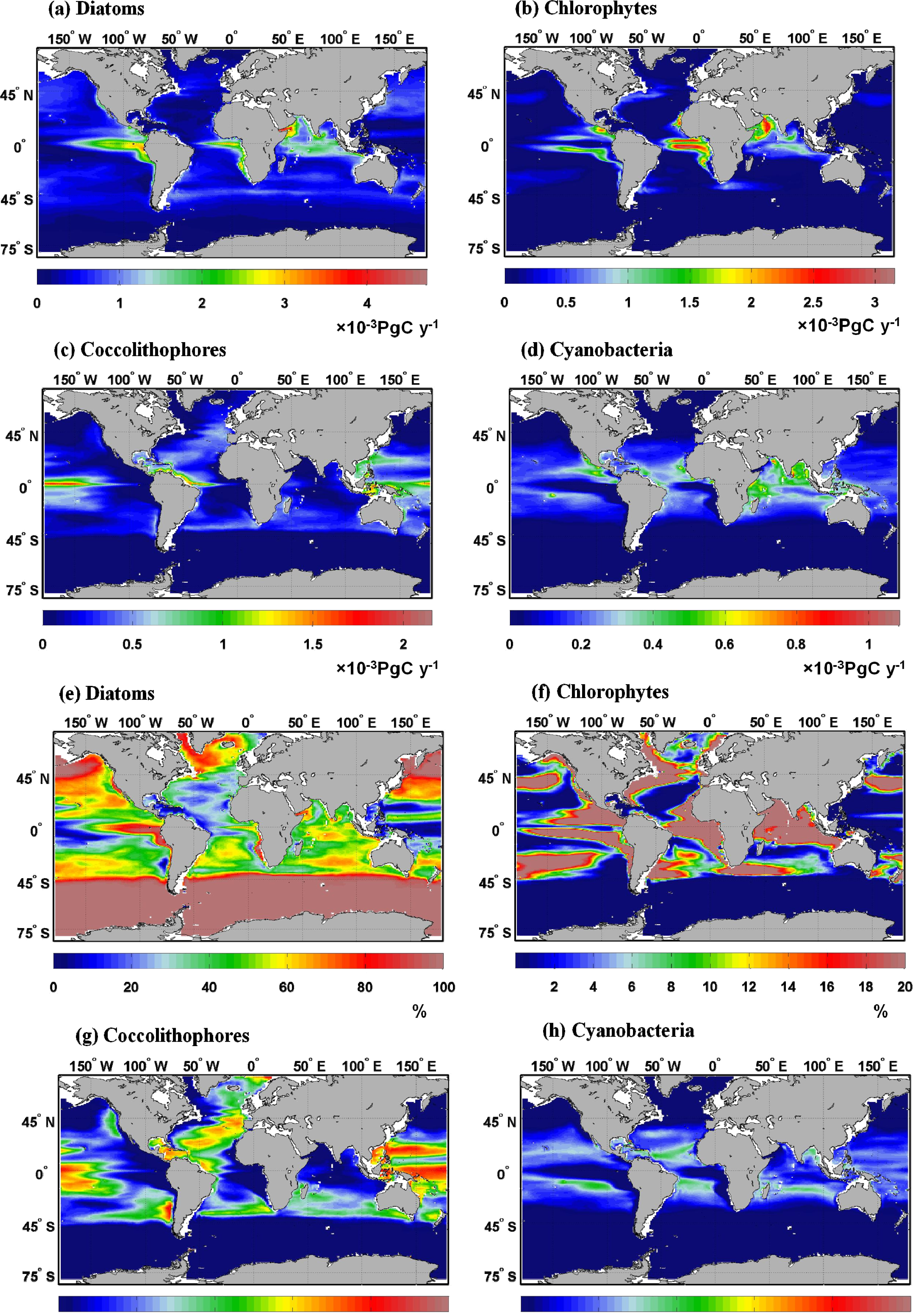
2.1. Climatology of Primary Production and Comparison with VGPM

Globally, the total primary production from the assimilated NOBM was 39 PgC·y−1, with the majority of this total production coming from the Equatorial Pacific (∼17% or 6.5 PgC·y−1) and the South and North Central Pacific (∼12%, Table 1). The Southern Ocean contributed the fourth most to the global primary production with 4.5 PgC (∼11%) produced annually. This estimate of total primary production at a global scale falls in the lower range of values previously reported by Carr et al. [22] in an intercomparison of 24 models. In Carr et al. [22], total primary production ranged between 40 and 60 PgC·y−1. This discrepancy can be explained by the fact that the northernmost latitude covered by NOBM is 72°N. Similarly to the spatial distribution of primary production in the NOBM, Carr et al. [22] found that most total primary production occurred in the Pacific Ocean (a total of 21 PgC·y−1 or 44% for the entire basin compared to 17 PgC·y−1 or 44% for the entire Pacific Ocean using the NOBM).
Carr et al. [22] compared the global primary production fields corresponding to 8 months of 1998 and 1999. Comparing one satellite-based approach with the NOBM for a longer period (1998–2011), we found that the primary production from the model was greater than the satellite-based approach (VGPM) by ∼6 PgC·y−1 (Figure 1).
The reason our global primary production using VGPM is lower than previously published values [25,26] is two-fold. (1) We have regridded the data so that it would be on the same grid as the NOBM and therefore comparing the same resolution. This turns out to be an important step since global averages can change because of small scale features that are smoothed out during regridding in order to make the VGPM comparable to the NOBM. (2) Since the NOBM does not include water shallower than 200 m and is restricted to 72°N and 84°S, we applied this mask to the VGPM data. This results in masking of coastal areas that are often high in primary productivity. Within the 12 regions, annual regional means from both approaches was always within ∼2 PgC·y−1 (Figures 2 and 3). The greatest difference was observed in the Equatorial regions (model between 1.4 and 2.3 PgC·y−1 higher than VGPM) and in the Southern Ocean (VGPM 1.2 PgC·y−1 higher than the model). In all regions except in the Southern Ocean, the North Pacific and North Atlantic, i.e., the high latitudes, primary production from the model was greater than that from the satellite-based approach.
Globally, diatoms were the group that contributed the most to the total phytoplankton production (∼50%, the equivalent of ∼20 PgC·y−1, Figure 4). Coccolithophores and chlorophytes each contributed to ∼20% (∼7 PgC·y−1) of the total primary production. Cyanobacteria represented about 10% (∼4 PgC·y−1) of the total primary production. Primary production by diatoms was highest in high latitudes (>40°) and in major upwelling systems (Equatorial Pacific and Benguela system, Figure 5a). In the Southern Ocean and the North Pacific, diatoms contributed more than 85% to the total primary production. The only region where diatoms contributed to <40% of the primary production was in the Equatorial Atlantic and the North Central Atlantic. Maximum primary production for chlorophytes occurred in regions directly adjacent to those regions where maximum primary production from diatoms was encountered (i.e., Equatorial Pacific and Benguela systems, Figure 5b) and in the Equatorial Indian. Coccolithophores contributed considerably to the total primary production in the North Central Atlantic (38%, see Table 1 for an equivalence in PgC·y−1 for all regions and groups) and Western Equatorial Pacific (31%). In the southern sub-polar regions (South Indian, South Pacific, South Atlantic), primary production by coccolithophores was ∼20%–30% of the total primary production. Some local high primary production by coccolithophores led to average >20% in the North Atlantic and North Central Pacific (Figure 5c). Finally, although globally cyanobacteria only contributed to ∼10% of the total primary production, their contribution reached ∼80% in the ocean gyres (Figure 5d).
Using a satellite-derived approach, Uitz et al. [17] estimated the global total primary production to be ∼46 PgC·y−1, which is 7 PgC·y−1 higher than NOBM (39 PgG·y−1). Except for the primary production by microphytoplankton, a similar tendency (satellite-derived approach higher than the NOBM) was found for the group-specific primary production: ∼15 PgC·y−1 for microphytoplankton (∼20 PgC·y−1 for NOBM), 20 PgC·y−1 (∼8 PgC·y−1 for NOBM) for nanophytoplankton and 11 PgC·y−1 (∼11 PgC·y−1 for NOBM) for picophytoplankton. In the satellite-derived approach, microphytoplankton were identified as “mostly diatoms” and, therefore, was close to the classification of the NOBM. In Uitz et al. [17], nanophytoplankton included prymnesiophytes, pelagophytes and cryptophytes and was therefore compared to coccolithophores (prymnesiophytes) from the NOBM. Picophytoplankton of the Uitz et al. [17] approach included cyanobacteria, prochlorophytes, chlorophytes and were, therefore, compared to the sum of cyanobacteria and chlorophytes from the NOBM. The group of nanophytoplankton, and to a lesser extent picophytoplankton, in the satellite-derived approach encompassed more groups than in the NOBM. In the NOBM, the sum of the group-specific primary production equals the total primary production. Although nominal, some of the differences between the two approaches can also be attributed to the difference in the depth of integration: primary production in the NOBM is calculated over the entire water column whereas the satellite-derived approach integrated over the upper water column (0–1.5 Zeu). This would lead to a higher primary production in the model than in the satellite-derived approach. The satellite-derived approach of Uitz et al. [17] was developed using data sets collected in case-1 waters only and therefore pixel in water shallower than 200 m were disregarded. Both approaches therefore do not take into account the primary production of coastal waters.
Uitz et al. [17] divided the global ocean into six basins and provided the size-specific primary production for those six basins as well as the breakdown numbers for the north and south of each basin. We can therefore compare these regions with the group-specific primary production from the NOBM. Regionally, the greatest difference (4.3 PgC·y−1) was observed for nanophytoplankton in the Pacific Ocean. For all the other regions (Atlantic, Pacific, Equatorial, Indian and Southern Ocean), the size/group-specific primary production from the two approaches was always within 3.5 PgC·y−1 of each other. As mentioned previously, the group of nanophytoplankton in the satellite-derived approach, and to a lesser extent picophytoplankton, encompassed more groups than in the NOBM. Therefore, it is expected that the estimates of primary production from the satellite-derived approach for this group would be greater than the one from the NOBM. By looking at individual regions, we can attempt to narrow down the reasons, other than the classification difference described earlier, why the satellite-derived approach was globally higher than the NOBM (nothing changed just need to check this sentence). If we compare the latitudes between 10°S and 10°N, we find that except for nanophytoplankton, the total and the primary production by micro- and picophytoplankton using the NOBM was higher than those from the satellite-derived approach (by 2.3–2.4 PgC·y−1). This is the opposite of what was observed at a global scale. This suggests that the reasons behind the global satellite-derived approach having larger estimates than the NOBM may be related to the difference in coverage. The northernmost latitude covered by the NOBM being 72°N would lead to a global underestimate of total and group-specific primary production using NOBM, as was observed for total, nano- and picophytoplankton primary production. Some of the discrepancies between the two approaches may also be linked to the inherent sampling bias resulting from clouds, thick aerosols, interorbit gaps, sunglint and high solar zenith angle in the satellite-derived approach. This sampling bias can lead to 6%–8% annual mean bias [27] with the largest bias caused by the exclusion of data with high solar zenith angle. Aerosol-related sampling biases occur in regions such as North Indian, Equatorial Atlantic, etc., which unfortunately were not regions for which Uitz et al. [17] reported size-specific primary production values.

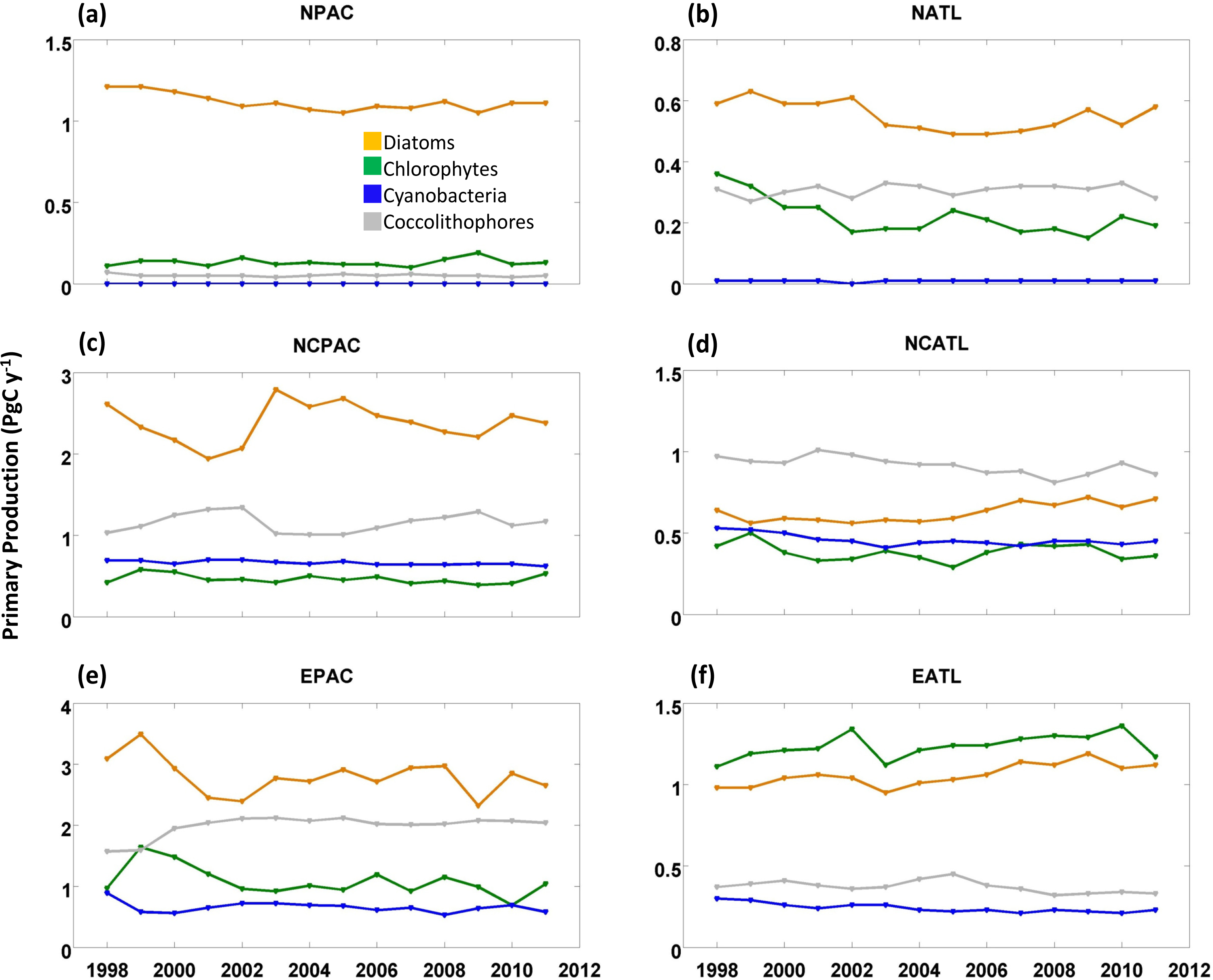
2.2. Interannual Variability

Globally the magnitude of interannual variability was of maximum 3 PgC·y−1 which compares favorably with the previous estimates of an average magnitude of 2 PgC·y−1 based on a period from 1992 to 2010 [28]. Over the period 1998–2011, the relative contribution of each phytoplankton group to the total primary production varied by ∼4% except for cyanobacteria, for which the highest interannual variability was of only ∼2%. This was the equivalent of ∼2 PgC·y−1 for diatoms and chlorophytes and ∼1 PgC·y−1 for cyanobacteria and coccolithophores. In both the Atlantic and the Pacific, the interannual variability in group-specific primary production increased at low latitude (Figure 6).
The region where all groups displayed the greatest interannual variation was the Equatorial Pacific (Figure 6). Here, the magnitude of interannual variability in primary production by diatoms and chlorophytes was ∼1 PgC·y−1 and 0.3–0.4 PgC·y−1 for cyanobacteria and coccolithophores, respectively. Phytoplankton composition in the Equatorial Pacific is known to be strongly influenced by climate variability. Numerous studies have shown the impact of climate variability in this region [2932]. Rousseaux & Gregg [15] reported a phytoplankton composition shift in this region during the transition from El Niño to La Niña conditions. The group-specific primary production followed a similar pattern (Figure 6) with diatoms and chlorophytes reaching their maximum primary production in 1999 (La Niña) while primary production by cyanobacteria was at its maximum in 1998 (El Niño).
Interannual variability in group-specific primary production was also high in the North Central Pacific (Figure 6). Here, the magnitude over which the primary production varied was comparable to that found in the Equatorial Pacific for diatoms (∼0.85 PgC·y−1) but was lower for the other 3 groups (0.10–0.30 PgC·y−1).
By using climate indices, we can assess the factors driving this interannual variability. The MEI attempts to characterize climate variability using six relevant atmospheric and ocean variables (sea-level pressure, surface wind vector, sea surface temperature, surface air temperature, and total cloudiness fraction [33]). The MEI has been widely used in assessing the effects of climate variability on ocean biology [3438]. Positive values of MEI represent the warm ENSO phase (e.g., El Niño phase) while negative values represent the cold ENSO phase (e.g., La Niña). Globally, the primary production of all groups except coccolithophores were significantly correlated with the Multivariate El Niño Index (MEI). Behrenfeld et al. [38] showed that for the permanently stratified ocean (between 40°S and 40°N) there was a significant correlation between primary production and MEI. Dave and Loizier [39] attributed this correlation between primary production and MEI across all of the permanently stratified oceans to be dominated by the correlation in the Equatorial Pacific. Regionally, there was a significant correlation between the MEI and the primary production from the NOBM for 2 phytoplankton groups or more in 7 out of the 12 regions (Table 2). In the Equatorial Pacific for example, primary production by cyanobacteria was significantly (p < 0.05) positively correlated while primary production by diatoms and chlorophytes were negatively correlated. This was similar to the changes in phytoplankton composition that have been reported for this region: during El Niño (positive MEI) the upwelling of nutrient rich waters is suppressed and leads to a shift from a community dominated by diatoms to a community dominated by cyanobacteria [15]. In the North Central Pacific, primary production by chlorophytes and diatoms were significantly correlated with MEI, but here diatoms were positively correlated while chlorophytes were negatively correlated. Unlike the Equatorial Pacific, there is no feature like the upwelling tongue here. Instead, this region is more biogeographically diverse with a large central gyre bounded by regions of modest to large productivity at the lateral and northern margins.
In the Atlantic Ocean, all 4 regions except the Equatorial Atlantic had two or more phytoplankton groups whose primary production was significantly correlated to MEI. In the South Atlantic, diatoms and chlorophytes were negatively correlated and cyanobacteria positively correlated with MEI. In the North and North Central Atlantic, primary production by coccolithophores was significantly positively correlated to MEI while primary production by cyanobacteria was significantly negatively correlated with the MEI. In the North Atlantic, physical forcing that impact the vertical stability of the water column has been shown to be the largest factor determining the timing and magnitude of the spring bloom [40,41]. Shutler et al. [42] showed that the surface area covered by coccolithophores (Emiliania huxleyi) in the North Atlantic was strongly positively correlated with ENSO climate oscillation (r = 0.75, p < 0.02). The variability in the coverage of coccolithophores has important consequences in the carbon cycle leading to an average reduction in the monthly air-sea flux of ∼55% in regions where blooms are prevalent [42]. It has also been shown that >89% of the variability in the E. huxleyi coverage is explained by variation in physical conditions of solar radiation, mixed layer depth and water temperature [43]. In the North and North Central Atlantic, El Niño conditions seem to promote increasing primary productivity of coccolithophores through changes of physical forcing. These physical connections between MEI and the northern Atlantic remain, however, difficult to verify and therefore statistical noise cannot be ruled out.
Some of the regions such as the North Atlantic, the Pacific Ocean and the Southern Ocean have well established climate indices. In the Southern Ocean for example, the Southern Annular Mode (SAM) is the dominant climate pattern. It is defined as the leading mode of Empirical Orthogonal Function analysis of monthly atmospheric pressure gradient. It has been suggested that a positive SAM, characterized by stronger westerly wind anomaly would intensify the upwelling therefore resulting in an increase in phytoplankton biomass [44]. Arrigo et al. [45] found a significant correlation between SAM and SST in the Southern Ocean. In this region, the MEI was not correlated to the primary production for any groups (Table 2) and SAM was only correlated to chlorophytes (Table 3). Similarly, Arrigo et al. [45] found that only 31% of the variation in annual primary production could be explained by SAM index. Instead, Arrigo et al. [45] found that most of the interannual variability in primary production was driven by changes in sea ice cover. Although changes in surface nutrient induced by processed associated with atmospheric variability (e.g., SAM) are also likely to play a role, especially at regional scales through enhanced upwelling, it seems that its effect is relatively limited on both the total and group-specific primary production in this region.
The North Atlantic Oscillation index (NAO) is calculated as the normalized sea level pressure difference between the Azores and Iceland [46]. When the NAO is high, the westerlies are stronger than average, which in turn transport warm and moist air toward Europe. In the North Central Atlantic, a positive NAO was associated with significantly less primary production by diatoms and significantly more by cyanobacteria (Table 3). A few local scale studies have shown a positive correlation between NAO and phytoplankton concentration [4750] as well as a phytoplankton composition shift from a diatom-dominated community during positive NAO to a dinoflagellates-dominated community during negative phase of NAO in the North Atlantic [51]. At the Bermuda Atlantic Time Series station (North Central Pacific in this paper), Bates et al. [52] found that high NAO was associated with a warming of the subtropical gyre and decreasing MLD and primary production. The decrease in mixed layer depth in this region and the warming of the subtropical gyre are conditions that are not favorable for the growth of diatoms and may therefore explain the significant negative relationship between NAO and the primary production from diatoms. These conditions on the other hand are favorable for the growth of cyanobacteria and support the significant positive relationship observed between the NAO and primary production of cyanobacteria in this region. Further north, in the North Atlantic, a significant negative correlation was found between NAO and primary production by chlorophytes and coccolithophores, but no correlation was found with the primary production from cyanobacteria and diatoms. As noted by Racault et al. [53] the effects of NAO on the North and North Central Atlantic are mixed. They describe the NAO influence on sea surface temperature as a tripole pattern with the subpolar gyre (north of 55°N) and the southern part of the subtropical gyre (south of 25°N) being positively correlated with the NAO while the western part of the subtropical gyre being negatively correlated. At a basin scale, Leterme et al. [54] showed that the influence of NAO on diatoms and dinoflagellates abundance was highly mixed across the North Atlantic basin. In the North Atlantic, positive NAO has been associated with enhanced sea-ice production and reduced stratification [55]. This in turns deepens the mixed layer depth, delaying the initiation of phytoplankton growth, reducing the chlorophyll maxima [41,56] and shortening the duration of the bloom [53]. This suggests that the NAO index has different effects on the biogeochemical cycles, including the primary production, in these different regions. Finally, both the MEI and NAO agreed on the limited effect of climate variability on group-specific primary production in the Equatorial Atlantic, both indices diverged on the effect of climate variability on the group-specific primary production in the North, North Central and South Atlantic (Tables 2 and 3). This is not totally unexpected since in contrast to the MEI, the NAO is largely an atmospheric mode.
The Pacific Decadal Oscillation [57] is an index of oceanic climate variability with a similar expression to El Niño, but acting on a longer time scale. It is defined as the leading principal component of surface temperature variability north of 20°N. During the positive phase of the PDO, trade winds generally weaken reducing the upwelling of nutrient-rich water. Using the PDO, we found that phytoplankton primary production correlations with this index in the North Central Pacific were the same as for the MEI (positive for diatom production and negative for chlorophytes). In the North Pacific however, the PDO was negatively correlated with chlorophytes and cyanobacteria whereas there was no significant correlation between the MEI and any of the group-specific primary production. These two climate phenomenon can vary independently and exhibit variable strength in both the warm and cold phase [33,58]. Corno et al. [59] suggested that the different timescale of ENSO and PDO would likely confound direct relationships. Several studies have shown a correlation between climate variability and chlorophyll concentration as well as primary production in the Pacific [5962]. Chiba et al. [63] found a significant correlation between PDO and the timing of the annual bloom in the western North Pacific (average date occurring in mid-May) but could not find a relationship between the interannual variation of the summertime phytoplankton community structure and the PDO. Karl et al. [62,64] found that during a positive phase of the PDO (1965–1977), the plankton community composition shifted with prokaryotes becoming more dominant and coincided with changing new and export production, nutrient supply and fisheries yields.
In the Equatorial Pacific, there was a significant positive correlation between both MEI and PDO and the primary production by cyanobacteria and a negative correlation for the production by diatoms. Climate variability seemed to have only a limited effect on the primary production in the South Pacific. Here, there was a significant correlation between the PDO and the primary production only by diatoms. The effects of climate variability in the South Pacific remain poorly characterized. For this region, Thomas et al. [60] suggested some correlation between PDO and coastal chlorophyll at least at specific latitudes. The effects that PDO has on the phytoplankton composition and productivity are similarly poorly characterized. Furthermore, since the PDO is a decadal scale phenomena, the satellite observations currently available do not cover a period long enough to identify possible relationships between PDO and phytoplankton dynamics (whether in terms of composition or primary production).

3. Experimental Section

Global primary production is derived from an established coupled ocean biogeochemical model, the NASA Ocean Biogeochemical Model [65]. It is a three-dimensional representation of circulation/biogeochemical/radiative processes in a domain that spans from −84° to 72° at a 1.25° resolution in water deeper than 200 m. NOBM is coupled with the Poseidon ocean general circulation model, which is driven by wind stress, sea surface temperature, and shortwave radiation [65]. The model includes 3 detrital pools (silica, N/C and iron detritus), 4 phytoplankton groups (diatoms, coccolithophores, chlorophytes and cyanobacteria) and 4 nutrients (ammonium, nitrate, iron and silicate). The phytoplankton groups differ in their maximum growth rates, sinking rates, nutrient requirements, and optical properties.
Satellite ocean chlorophyll from SeaWiFS and MODIS-Aqua for the years 1998–2012 is assimilated into NOBM following Gregg [66]. Multi-variate nutrient adjustments corresponding to the chlorophyll assimilation [15] are also included. Bias-correction of the satellite chlorophyll data is performed prior to assimilation using public in situ archives in the Empirical Satellite Radiance-In situ Data (ESRID) methodology [67]. The ESRID method also has the attribute of reducing discontinuities between the two satellite data sets [68]. The time series uses SeaWiFS data from 1998 to 2002, then switches to MODIS-Aqua data.
Primary production is computed in the model as a function of growth rate multiplied by the carbon: chlorophyll ratio:
PP = μ i C i Φ dz
where μi is the growth rate of phytoplankton component i, Ci is the chlorophyll concentration of component i, Φ is the carbon:chlorophyll ratio, and the product is integrated over depth. It is a diagnostic variable in the model, representing the integral of net carbon uptake in the water column. Photoadaptation is simulated by stipulating three states: 50, 150, and 200 (mmol·quanta·m−2·s−1). This is based on laboratory studies, which typically divide experiments into low, medium, and high classes of light adaptation [65]. Carbon:chlorophyll ratios (Φ) correspond to the photoadaptation state, to represent the tendency of phytoplankton to preferentially synthesize chlorophyll in low light conditions, to enable more efficient photon capture. The three Φ states corresponding to the three light states are 25, 50, and 80 g·g−1. For irradiance levels falling between the three light states, the C: chl ratios are linearly interpolated.
Irradiance data to drive phytoplankton growth is taken from the Ocean-Atmosphere Spectral Irradiance Model [69] for the years of interest. This model computes spectral irradiance in 33 bands for the domain 200 nm to 4 μm, at the ocean surface as a function of atmospheric optical properties [69], and then propagates the spectral irradiance downward and upward through the water column as a function of ocean optical properties [70,71]. Surface spectral irradiance and photosynthetically available irradiance data are publicly available at gmao.gsfc.nasa.gov/research/oceanbiology/data.php.
Climate indices were downloaded from the NOAA Climate Prediction Center ( http://www.cpc.ncep.noaa.gov).

4. Conclusions

To our knowledge, this paper represents the first attempt at estimating taxonomic/functional group-specific primary production at a global scale. Globally, diatoms contributed the most to the total phytoplankton production (∼50%) followed by coccolithophores and chlorophytes (∼20%) and cyanobacteria (10%). Primary production by diatoms was highest in the high latitudes (>40°) and in major upwelling systems (Equatorial Pacific and Benguela system). These results provide a modeling and data assimilation perspective to phytoplankton partitioning of primary production and contribute to our understanding of the dynamics of the carbon cycle in the oceans at a global scale. Although the comparison with group-specific primary production derived from the satellite approach was complicated by differences in methodology and classification, it is reassuring that the two approaches agreed on the overall distribution. The continuous improvements of biogeochemical models will ultimately allow for not only prediction, but also sensitivity analyses, which could potentially improve our understanding of the forcing factors of primary production. Since the forcing factors for primary production are likely to be different for each phytoplankton groups, these sensitivity analyses conducted with a model that allows for the discrimination among phytoplankton groups may in the future improve our understanding of the biogeochemical cycles in the oceans.
In this paper, we have also made a first step towards the understanding of climate forcing indices on primary production by analyzing the statistical correlation between group specific primary production and various climate indices. The lack of in situ data on group-specific primary production does limit our ability to assess the bias and uncertainty in the group-specific primary production from NOBM. The greatest interannual variability in primary production was observed in the Equatorial Pacific. The SAM index in the Southern Ocean was not correlated to any group-specific primary production and agrees with previous findings [45] that showed interannual variability in primary production in this region to be mostly driven by changes in ice cover. In the Atlantic and Pacific, the effects of NAO and PDO on phytoplankton dynamics remain divided. While the current research on MEI and phytoplankton dynamics seems to mostly agree, there is a lot more divergence when looking at index that are either representing largely an atmospheric mode (e.g., NAO) or longer time scale (e.g., decadal, PDO).

Acknowledgments

We thank the NASA Ocean Color project for providing the satellite chlorophyll data and the NASA Center for Climate Simulation for computational support. We also thank the Ocean Productivity website for providing the VGPM data ( www.science.oregonstate.edu). This paper was funded by the NASA EOS, MAP, and CMS Programs.

Conflicts of Interest

The authors declare no conflict of interest.

References

  1. Behrenfeld, M.J.; Randerson, J.T.; McClain, C.R.; Feldman, G.C.; Los, S.O.; Tucker, C.J.; Falkowski, P.G.; Field, C.B.; Frouin, R.; Esaias, W.E. Biospheric primary production during an enso transition. Science 2001, 291, 2594–2597. [Google Scholar]
  2. Ciotti, A.M.; Lewis, M.R.; Cullen, J.J. Assessment of the relationships between dominant cell size in natural phytoplankton communities and the spectral shape of the absorption coefficient. Limnol. Oceanogr 2002, 47, 404–417. [Google Scholar]
  3. Mouw, C.B.; Yoder, J.A. Optical determination of phytoplankton size composition from global seawifs imagery. J. Geophys. Res 2006, 115, C12018. [Google Scholar]
  4. Alvain, S.; Moulin, C.; Dandonneau, Y.; Bréon, F.M. Remote sensing of phytoplankton groups in case 1 waters from global seawifs imagery. Deep Sea Res. Part I: Oceanogr. Res. Papers 2005, 52, 1989–2004. [Google Scholar]
  5. Uitz, J.; Claustre, H.; Morel, A.; Hooker, S.B. Vertical distribution of phytoplankton communities in open ocean: An assessment based on surface chlorophyll. J. Geophys. Res 2006, 111, C08005. [Google Scholar]
  6. Aiken, J.; Fishwick, J.R.; Lavender, S.; Barlow, R.; Moore, G.F.; Sessions, H.; Bernard, S.; Ras, J.; Hardman-Mountford, N.J. Validation of meris reflectance and chlorophyll during the bencal cruise october 2002: Preliminary validation of new demonstration products for phytoplankton functional types and photosynthetic parameters. Int. J. Remote Sens 2007, 28, 497–516. [Google Scholar]
  7. Dutkiewicz, S.; Follows, M.J.; Bragg, J.G. Modeling the coupling of ocean ecology and biogeochemistry. Glob. Biogeochem. Cy 2009, 23, GB4017. [Google Scholar]
  8. Le Quere, C.; Harrison, S.P.; Colin Prentice, I.; Buitenhuis, E.T.; Aumont, O.; Bopp, L.; Claustre, H.; Cotrim Da Cunha, L.; Geider, R.; Giraud, X.; et al. Ecosystem dynamics based on plankton functional types for global ocean biogeochemistry models. Glob. Chang. Biol 2005, 11, 2016–2040. [Google Scholar]
  9. Moore, J.K.; Doney, S.C.; Lindsay, K. Upper ocean ecosystem dynamics and iron cycling in a global three-dimensional model. Glob. Biogeochem. Cy 2004, 18, GB4028. [Google Scholar]
  10. Dunne, J.P.; Armstrong, R.A.; Gnanadesikan, A.; Sarmiento, J.L.; Slater, R.D. Empirical and mechanistic models for the particle export ratio. Glob. Biogeochem. Cy 2005, 19, GB4026. [Google Scholar]
  11. Doney, S.C.; Ducklow, H.W. A decade of synthesis and modeling in the us joint global ocean flux study. Deep Sea Res. Part II: Top. Stud. Oceanogr 2006, 53, 451–458. [Google Scholar]
  12. Hirata, T.; Hardman-Mountford, N.J.; Barlow, R.; Lamont, T.; Brewin, R.; Smyth, T.; Aiken, J. An inherent optical property approach to the estimation of size-specific photosynthetic rates in eastern boundary upwelling zones from satellite ocean colour: An initial assessment. Prog. Oceanogr 2009, 83, 393–397. [Google Scholar]
  13. Dandonneau, Y.; Deschamps, P.-Y.; Nicolas, J.-M.; Loisel, H.; Blanchot, J.; Montel, Y.; Thieuleux, F.; Bécu, G. Seasonal and interannual variability of ocean color and composition of phytoplankton communities in the north atlantic, equatorial pacific and south pacific. Deep Sea Res. Part II: Top. Stud. Oceanogr 2004, 51, 303–318. [Google Scholar]
  14. Masotti, I.; Moulin, C.; Alvain, S.; Bopp, L.; Tagliabue, A.; Antoine, D. Large-scale shifts in phytoplankton groups in the equatorial pacific during enso cycles. Biogeosciences 2011, 8, 539–550. [Google Scholar]
  15. Rousseaux, C.S.; Gregg, W.W. Climate variability and phytoplankton composition in the pacific ocean. J. Geophys. Res 2012, 117, C10006. [Google Scholar]
  16. Martinez, E.; Antoine, D.; D’Ortenzio, F.; Gentili, B. Climate-driven basin-scale decadal oscillations of oceanic phytoplankton. Science 2009, 326, 1253–1256. [Google Scholar]
  17. Uitz, J.; Claustre, H.; Gentili, B.; Stramski, D. Phytoplankton class-specific primary production in the world’s oceans: Seasonal and interannual variability from satellite observations. Glob. Biogeochem. Cy 2010, 24, GB3016. [Google Scholar]
  18. Kameda, T.; Ishizaka, J. Size-fractionated primary production estimated by a two-phytoplankton community model applicable to ocean color remote sensing. J. Oceanogr 2005, 61, 663–672. [Google Scholar]
  19. Brewin, R.J.; Lavender, S.J.; Hardman-Mountford, N.J. Mapping size-specific phytoplankton primary production on a global scale. J. Maps 2010, 6, 448–462. [Google Scholar]
  20. Morel, A. Light and marine photosynthesis: A spectral model with geochemical and climatological implications. Prog. Oceanogr 1991, 26, 263–306. [Google Scholar]
  21. Friedrichs, M.A.M.; Carr, M.E.; Barber, R.T.; Scardi, M.; Antoine, D.; Armstrong, R.A.; Asanuma, I.; Behrenfeld, M.J.; Buitenhuis, E.T.; Chai, F.; et al. Assessing the uncertainties of model estimates of primary productivity in the tropical pacific ocean. J. Mar. Syst 2009, 76, 113–133. [Google Scholar]
  22. Carr, M.E.; Friedrichs, M.A.M.; Schmeltz, M.; Noguchi Aita, M.; Antoine, D.; Arrigo, K.R.; Asanuma, I.; Aumont, O.; Barber, R.; Behrenfeld, M.; et al. A comparison of global estimates of marine primary production from ocean color. Deep Sea Res. Part II: Top. Stud. Oceanogr 2006, 53, 741–770. [Google Scholar] [Green Version]
  23. Saba, V.S.; Friedrichs, M.A.M.; Carr, M.E.; Antoine, D.; Armstrong, R.A.; Asanuma, I.; Aumont, O.; Bates, N.R.; Behrenfeld, M.J.; Bennington, V.; et al. Challenges of modeling depth-integrated marine primary productivity over multiple decades: A case study at bats and hot. Glob. Biogeochem. Cy 2010, 24, GB3020. [Google Scholar]
  24. Behrenfeld, M.J.; Falkowski, P.G. Photosynthetic rates derived from satellite-based chlorophyll concentration. Limnol. Oceanogr 1997, 42, 1–20. [Google Scholar]
  25. Behrenfeld, M.J.; Boss, E.; Siegel, D.A.; Shea, D.M. Carbon-based ocean productivity and phytoplankton physiology from space. Glob. Biogeochem. Cy 2005, 19, 14. [Google Scholar]
  26. Field, C.B.; Behrenfeld, M.J.; Randerson, J.T.; Falkowski, P. Primary production of the biosphere: Integrating terrestrial and oceanic components. Science 1998, 281, 237. [Google Scholar]
  27. Gregg, W.W.; Casey, N.W. Sampling biases in modis and seawifs ocean chlorophyll data. Remote Sens. Environ 2007, 111, 25–35. [Google Scholar]
  28. Chavez, F.P.; Messié, M.; Pennington, J.T. Marine primary production in relation to climate variability and change. Annu. Rev. Mar. Sci 2011, 3, 227–260. [Google Scholar]
  29. Chavez, F.P.; Strutton, P.G.; Friederich, G.E.; Feely, R.A.; Feldman, G.C.; Foley, D.G.; McPhaden, M.J. Biological and chemical response of the equatorial pacific ocean to the 1997–98 el niño. Science 1999, 286, 2126–2131. [Google Scholar]
  30. Wang, X.; Christian, J.R.; Murtugudde, R.; Busalacchi, A.J. Ecosystem dynamics and export production in the central and eastern equatorial pacific: A modeling study of impact of ENSO. Geophys. Res. Lett 2005, 32, L02608. [Google Scholar]
  31. Strutton, P.G.; Chavez, F.P. Primary productivity in the equatorial pacific during the 1997–1998 el niño. J. Geophys. Res 2000, 105, 20089–26101. [Google Scholar]
  32. Feely, R.A.; Boutin, J.; Cosca, C.E.; Dandonneau, Y.; Etcheto, J.; Inoue, H.Y.; Ishii, M.; Quéré, C.L.; Mackey, D.J.; McPhaden, M.; et al. Seasonal and interannual variability of co2 in the equatorial pacific. Deep Sea Res. Part II: Top. Stud. Oceanogr 2002, 49, 2443–2469. [Google Scholar]
  33. Wolter, K.; Timlin, M.S. Measuring the strength of enso events: How does 1997/98 rank? Weather 1998, 53, 315–324. [Google Scholar]
  34. Matsumoto, K.; Furuya, K. Variations in phytoplankton dynamics and primary production associated with enso cycle in the western and central equatorial pacific during 1994–2003. J. Geophys. Res 2011, 116, C12042. [Google Scholar]
  35. Villanoy, C.L.; Cabrera, O.C.; Yniguez, A.; Camoying, M.; de Guzman, A.; David, L.T.; Flament, P. Monsoon-driven coastal upwelling off zamboanga peninsula, philippines. Oceanography 2011, 24, 156–165. [Google Scholar]
  36. Dave, A.C.; Lozier, M.S. Local stratification control of marine productivity in the subtropical north pacific. J. Geophys. Res 2010, 115, C12032. [Google Scholar]
  37. Kostadinov, T.S.; Siegel, D.A.; Maritorena, S. Global variability of phytoplankton functional types from space: Assessment via the particle size distribution. Biogeosci. Discuss 2010, 7, 4295–4340. [Google Scholar]
  38. Behrenfeld, M.J.; O’Malley, R.T.; Siegel, D.A.; McClain, C.R.; Sarmiento, J.L.; Feldman, G.C.; Milligan, A.J.; Falkowski, P.G.; Letelier, R.M.; Boss, E.S. Climate-driven trends in contemporary ocean productivity. Nature 2006, 444, 752–755. [Google Scholar]
  39. Dave, A.C.; Lozier, M.S. Examining the global record of interannual variability in stratification and marine productivity in the low-latitude and mid-latitude ocean. J. Geophys. Res 2013, 118, 3114–3127. [Google Scholar]
  40. Follows, M.J.; Dutkiewicz, S.W. Meteorological modulation of the north atlantic spring bloom. Deep Sea Res. Part II: Top. Stud. Oceanogr 2002, 49, 321–344. [Google Scholar]
  41. Henson, S.A.; Robinson, I.; Allen, J.T.; Waniek, J.J. Effect of meteorological conditions on interannual variability in timing and magnitude of the spring bloom in the irminger basin, north atlantic. Deep Sea Res. Part I: Oceanogr. Res. Papers 2006, 53, 1601–1615. [Google Scholar]
  42. Shutler, J.; Land, P.; Brown, C.; Findlay, H.; Donlon, C.; Medland, M.; Snooke, R.; Blackford, J. Coccolithophore surface distributions in the north atlantic and their modulation of the air-sea flux of CO2 from 10 years of satellite earth observation data. Biogeosciences 2013, 10, 2699–2709. [Google Scholar]
  43. Raitsos, D.E.; Lavender, S.J.; Pradhan, Y.; Tyrrell, T.; Reid, P.C.; Edwards, M. Coccolithophore bloom size variation in response to the regional environment of the subarctic north atlantic. Limnol. Oceanogr 2006, 51, 2122–2130. [Google Scholar]
  44. Lovenduski, N.S.; Gruber, N. Impact of the southern annular mode on southern ocean circulation and biology. Geophys. Res. Lett 2005, 32, L11603. [Google Scholar]
  45. Arrigo, K.R.; van Dijken, G.L.; Bushinsky, S. Primary production in the southern ocean, 1997–2006. J. Geophys. Res 2008, 113, L19603. [Google Scholar]
  46. Hurrell, J.W. Decadal trends in the north atlantic oscillation. Science 1995, 269, 676–679. [Google Scholar]
  47. Weyhenmeyer, G.A.; Blenckner, T.; Petterson, K. Changes of the plankton spring outburst related to the north atlantic oscillation. Limnol. Oceanogr 1999, 44, 1788–1792. [Google Scholar]
  48. Irigoien, X.; Harris, R.P.; Head, R.N.; Harbour, D. North atlantic oscillation and spring bloom phytoplankton composition in the english channel. J. Plankton Res 2000, 22, 2367–2371. [Google Scholar]
  49. Reid, P.C.; Edwards, M.; Hunt, H.G.; Warner, A.J. Phytoplankton change in the north atlantic. Nature 1998, 391, 546–546. [Google Scholar]
  50. Sameoto, D. Decadal changes in phytoplankton color index and selected calanoid copepods in continuous plankton recorder data from the scotian shelf. Can. J. Fish. Aquat. Sci 2001, 58, 749–761. [Google Scholar]
  51. Henson, S.; Lampitt, R.; Johns, D. Variability in phytoplankton community structure in response to the north atlantic oscillation and implications for organic carbon flux. Limnol. Oceanogr 2012, 57, 1591–1601. [Google Scholar]
  52. Bates, N.R. Interannual variability of oceanic co2 and biogeochemical properties in the western North Atlantic subtropical gyre. Deep Sea Res. Part II: Top. Stud. Oceanogr 2001, 48, 1507–1528. [Google Scholar]
  53. Racault, M.-F.; Le Quéré, C.; Buitenhuis, E.; Sathyendranath, S.; Platt, T. Phytoplankton phenology in the global ocean. Ecol. Indic 2012, 14, 152–163. [Google Scholar]
  54. Leterme, S.C.; Edwards, M.; Seuront, L.; Attrill, M.; Reid, P.; John, A. Decadal basin-scale changes in diatoms, dinoflagellates, and phytoplankton color across the north atlantic. Limnol. Oceanogr 2005, 50, 1244–1253. [Google Scholar]
  55. Hu, A.; Rooth, C.; Bleck, R.; Deser, C. Nao influence on sea ice extent in the Eurasian coastal region. Geophys. Res. Lett 2002, 29, 2053–2056. [Google Scholar]
  56. Henson, S.A.; Dunne, J.P.; Sarmiento, J.L. Decadal variability in North Atlantic phytoplankton blooms. J. Geophys. Res 2009, 114, C04013. [Google Scholar]
  57. Mantua, N.J.; Hare, S.R. The pacific decadal oscillation. J. Oceanogr 2002, 58, 35–44. [Google Scholar]
  58. Mantua, N.J.; Hare, S.R.; Zhang, Y.; Wallace, J.M.; Francis, R.C. A pacific interdecadal climate oscillation with impacts on salmon production. Bull. Am. Meteorol. Soc 1997, 78, 1069–1079. [Google Scholar]
  59. Corno, G.; Karl, D.M.; Church, M.J.; Letelier, R.M.; Lukas, R.; Bidigare, R.R.; Abbott, M.R. Impact of climate forcing on ecosystem processes in the North Pacific subtropical gyre. J. Geophys. Res 2007, 112, C04021. [Google Scholar]
  60. Thomas, A.C.; Brickley, P.; Weatherbee, R. Interannual variability in chlorophyll concentrations in the humboldt and california current systems. Prog. Oceanogr 2009, 83, 386–392. [Google Scholar]
  61. Karl, D.M.; Bidigare, R.R.; Letelier, R.B. Sustained and aperiodic variability in organic matter production and phototrophic microbial community structure in the north pacific subtropical gyre. In Phytoplankton Productivity: Carbon Assimilation in Marine and Freshwater Ecosystems; Le B. Williams, P.J., Thomas, D.N., Reynolds, C.S., Eds.; Blackwell Science: Hoboken, NJ, USA, 2002; pp. 222–264. [Google Scholar]
  62. Karl, D.M.; Bidigare, R.R.; Letelier, R.M. Long-term changes in plankton community structure and productivity in the North Pacific subtropical gyre: The domain shift hypothesis. Deep Sea Res. Part II: Top. Stud. Oceanogr 2001, 48, 1449–1470. [Google Scholar]
  63. Chiba, S.; Batten, S.; Sasaoka, K.; Sasai, Y.; Sugisaki, H. Influence of the pacific decadal oscillation on phytoplankton phenology and community structure in the western north pacific. Geophys. Res. Lett 2012, 39, L15603. [Google Scholar]
  64. Karl, D.M. Minireviews: A sea of change: Biogeochemical variability in the north pacific subtropical gyre. Ecosystems 1999, 2, 181–214. [Google Scholar]
  65. Gregg, W.W.; Casey, N.W. Modeling coccolithophores in the global oceans. Deep Sea Res. Part II: Top. Stud. Oceanogr 2007, 54, 447–477. [Google Scholar]
  66. Gregg, W.W. Assimilation of seawifs ocean chlorophyll data into a three-dimensional global ocean model. J. Mar. Syst 2008, 69, 205–225. [Google Scholar]
  67. Gregg, W.W.; Casey, N.W.; O’Reilly, J.E.; Esaias, W.E. An empirical approach to ocean color data: Reducing bias and the need for post-launch radiometric re-calibration. Remote Sens. Environ 2009, 113, 1598–1612. [Google Scholar]
  68. Gregg, W.W.; Casey, N.W. Improving the consistency of ocean color data: A step toward climate data records. Geophys. Res. Lett 2010, 37, L04605. [Google Scholar]
  69. Gregg, W.W.; Casey, N.W. Skill assessment of a spectral ocean-atmosphere radiative model. J. Mar. Syst 2009, 76, 49–63. [Google Scholar]
  70. Aas, E. Two-stream irradiance model for deep waters. Appl. Opt 1987, 26, 2095–2101. [Google Scholar]
  71. Ackleson, S.G.; Balch, W.M.; Holligan, P.M. Response of water-leaving radiance to particulate calcite and chlorophyll a concentrations: A model for gulf of maine coccolithophore blooms. J. Geophys. Res 1994, 99, 7483–7499. [Google Scholar]
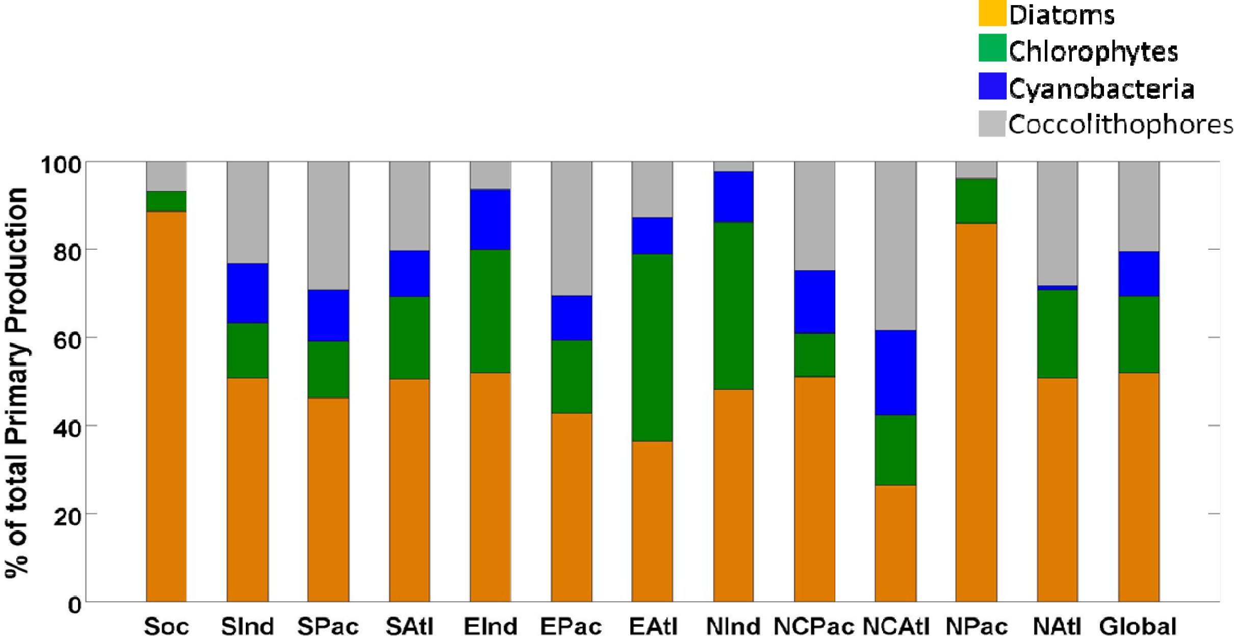
Figure 1. The 12 major oceanographic basins in the oceans.
Remotesensing 06 00001f1
Figure 2. Climatological map of primary production for (a) NOBM and (b) VGPM for the period from 1998 to 2011.
Remotesensing 06 00001f2
Figure 3. Difference between total primary production from NOBM and VGPM for the 12 basins and globally, averaged over the period from 1998 to 2011. See Table 1 for a list of abbreviations.
Remotesensing 06 00001f3
Figure 4. Global relative contributions of the four phytoplankton groups in NOBM to total primary production averaged over the period from 1998 to 2011. See Table 1 for a list of abbreviations.
Remotesensing 06 00001f4
Figure 5. Distribution of model class-specific primary production for the period from 1998 to 2011. (a–d) shows the primary production in absolute units. (e–h) shows the percent contribution of class-specific production to total primary production. Note the different scale for each plot.
Remotesensing 06 00001f5
Figure 6. Interannual variation of model class-specific primary production for diatoms, chlorophytes, cyanobacteria and coccolithophores in (a) North Pacific, (b) North Atlantic, (c) North Central Pacific, (d) North Central Atlantic, (e) Equatorial Pacific and (f) Equatorial Atlantic.
Remotesensing 06 00001f6
Table 1. Climatological primary production for the four phytoplankton groups in NOBM for 1998–2011, including relative contributions and total primary production.
DiatomsChlorophytesCyanobacteriaCoccolithophoresTotal
PgC·y−1%PgC·y−1%PgC·y−1%PgC·y−1%PgC·y−1
Southern Ocean (SOC)4.0890.250.000.374.5
South Indian (SIND)1.7510.4130.5130.8233.4
South Pacific (SPAC)2.2460.6130.6121.4294.7
South Atlantic (SATL)1.2510.4190.2100.5202.3
Equatorial Indian (EIND)1.9521.0280.5140.263.7
Equatorial Pacific (EPAC)2.8431.1160.7102.0316.5
Equatorial Atlantic (EATL)1.1361.2420.280.4132.9
North Indian (NIND)0.7480.6380.2120.021.5
North Central Pacific (NCPAC)2.4510.5100.7141.2254.7
North Central Atlantic (NCATL)0.6260.4160.5190.9392.4
North Pacific (NPAC)1.1860.1100.000.141.3
North Atlantic (NATL)0.6510.2200.010.3281.1
Global20.3526.8174.0108.02139.0
Table 2. Correlation coefficients between group-specific primary production and the Multivariate El Niño Index (MEI) in 12 major oceanographic basins. Bold and (*) indicates statistical significance (p < 0.05). See Table 1 for a list of abbreviations.
SOCSINDSPACSATLEINDEPACEATLNINDNCPACNCATLNPACNATL
Diatoms−0.12−0.14−0.10−0.17*−0.46*−0.68*−0.05−0.09*0.21*0.10*0.130.18*
Chlorophytes−0.13−0.09−0.06−0.17*−0.38*−0.28*−0.14−0.35*−0.18*0.06*0.010.00*
Cyanobacteria−0.050.00−0.070.33*0.13*0.61*0.100.18*0.03*−0.17*0.01−0.17*
Coccolithophores0.01−0.13−0.06−0.14*0.09*0.12*−0.140.18*0.08*0.23*0.120.15*
Table 3. Correlation coefficients between group-specific primary production and several region-specific climate indices: Antarctic Oscillation (AAO), North Atlantic Oscillation (NAO), and Pacific Decadal Oscillation (PDO). Bold and (*) indicates statistical significance (p < 0.05).
DiatomsChlorophytesCyanobacteriaCoccolithophores
AAOSouthern Ocean0.090.16*0.080.14
NAONorth Atlantic−0.11*−0.22*−0.09−0.25*
North Central Atlantic−0.17*−0.050.21*−0.12
Equatorial Atlantic−0.06−0.050.000.06
South Atlantic−0.020.12−0.22*0.14
PDONorth Pacific0.02−0.26*−0.19*−0.07
North Central Pacific0.40*−0.25*0.03−0.07
Equatorial Pacific−0.24*−0.130.45*0.17*
South Pacific−0.20*0.040.090.00

