Article

A New Approach for the Analysis of Hyperspectral Data: Theory and Sensitivity Analysis of the Moment Distance Method

by
Eric Ariel L. Salas
* and
Geoffrey M. Henebry
Geospatial Sciences Center of Excellence (GSCE), South Dakota State University, Brookings, SD 57007, USA
*
Author to whom correspondence should be addressed.
Remote Sens. 2014, 6(1), 20-41; https://doi.org/10.3390/rs6010020
Submission received: 1 November 2013 / Revised: 10 December 2013 / Accepted: 10 December 2013 / Published: 19 December 2013

Abstract

:
We present the Moment Distance (MD) method to advance spectral analysis in vegetation studies. It was developed to take advantage of the information latent in the shape of the reflectance curve that is not available from other spectral indices. Being mathematically simple but powerful, the approach does not require any curve transformation, such as smoothing or derivatives. Here, we show the formulation of the MD index (MDI) and demonstrate its potential for vegetation studies. We simulated leaf and canopy reflectance samples derived from the combination of the PROSPECT and SAIL models to understand the sensitivity of the new method to leaf and canopy parameters. We observed reasonable agreements between vegetation parameters and the MDI when using the 600 to 750 nm wavelength range, and we saw stronger agreements in the narrow red-edge region 720 to 730 nm. Results suggest that the MDI is more sensitive to the Chl content, especially at higher amounts (Chl > 40 μg/cm2) compared to other indices such as NDVI, EVI, and WDRVI. Finally, we found an indirect relationship of MDI against the changes of the magnitude of the reflectance around the red trough with differing values of LAI.

Graphical Abstract

1. Introduction

Over the past three decades, spectral indices have been devised to extract specific information for vegetation biophysical and biochemical properties. For instance, vegetation indices (VIs), usually formulated as a combinations of two or three spectral bands, use the concept of band ratio [14] and differences or weighted linear combinations [5,6] to make the most out of the contrasts in visible and NIR portions of the spectrum for measuring the photosynthetic activity of the plant [7,8] and exploring vegetation dynamics [913]. Studies have demonstrated that spectral VIs are correlated with vegetation parameters related to chlorophyll and biomass abundance [7,14,15].
The Normalized Difference Vegetation Index (NDVI) [4,16] exploits the strong differences in the red and NIR reflectances, where contrast in reflectance between vegetation and bare soil is maximal. It is calculated as the difference between the spectral reflectance measurements of the NIR and red bands divided by the sum of the same measurements. One drawback of the NDVI is its non-linear relationship with biophysical characteristics such as green Leaf Area Index (LAI) [17] and aboveground green biomass [18,19], and its sensitivity to soil background [2023]. Studies have shown the NDVI to asymptotically lose sensitivity under moderate to high biomass conditions and for certain ranges of LAI [2427]. This shortcoming of the NDVI had led to the development of derivatives and alternative indices. One example is the Wide Dynamic Range Vegetation Index (WDRVI) [6,28] that was initiated to enhance the dynamic range of the NDVI and later used for charactering vegetation dynamics [13,29,30] and estimating fractional vegetation cover [31].
We listed a number of VIs in Table 1. One apparent commonality among indices is their goal to minimize, if not diminish, the effects of external factors such as background and atmospheric conditions on spectral data [24]. Ratio-based indices, for instance the Modified Simple Ratio (MSR) [1] and the Transformed Vegetation Index (TVI) [32], are enhanced indices in terms of sensitivity to vegetation biophysical parameters. However, no technical distinction is seen between NDVI and TVI when it comes to detecting the active vegetation. In the TVI equation in Table 1, a ratio of less than 0.71 is deemed as non-vegetation and if it is greater than 0.7, it is considered vegetation.
In the soil-line-based VI category, the goal is to understand the behavior of indices [33]. Soil-distance-based VIs hope to cancel soil background effects [34], especially when vegetation cover is sparse [20]. The Perpendicular Vegetation Index (PVI) [35]; later modified as PVI1, PVI2 and PVI3 [36,37], was the first introduced VI based on the concept of the soil line. Other distance-based indices followed: the Difference Vegetation Index (DVI) [35], Green Vegetation Index (GVI) [38,39], and Weighted Difference Vegetation Index (WDVI) [5]. Gitelson et al. [40] looked into the two-dimensional spectral space defined by vegetation and soil lines and proposed indices to monitor vegetation fraction. The technique used focal points along the two lines to derive relationship ratios.
Optimized indices are combinations of concepts from slope-based and distance-based VIs. The Soil-Adjusted Vegetation Index (SAVI) [41], for instance, integrates the NDVI and the soil adjustment factor. Further enhancements resulted in a SAVI family of indices [36,42,43]. There have been remarkable inconsistencies in the logic with which the soil line has been utilized for specific vegetation indices. Bannari et al. ([44]) cited that the distance-based VIs are not consistent as to which band, red or NIR, is the independent variable in the regression equation.
Mathematical simplicity and ease of use are factors in choosing the vegetation index for a desired application. In this respect, ratio-based indices have an edge over their soil-distance-based VI counterparts. Although the optimized indices and distance-to-soil-line-based were successful in eliminating the atmospheric and soil background effects (e.g., WDVI [5]) or improving sensitivity to high biomass (e.g., [4547]), their application to monitoring vegetation at global scales is still disputed [48].
Limitations in the application of indices may include the choice of wavelength band positions and bandwidths [40]. Also, the indices are deficient in putting a focus on the shape of the curve. Whereas current indices incorporate two-band or three-band relations, no metric has dealt with the raw shape of the curve by featuring multiple bands that could carry additional spectral information useful for vegetation monitoring. In this era of spaceborne sensors such as the EO-1 Hyperion [49] and NASA’s Hyperspectral InfraRed Imager (HyspIRI) [5052] that may be launched in the future, VIs can be designed for optimal use of the spectrum by creating new indices that incorporate wavelengths not sampled by any broadband system [53]. Unlike broadband sensors such as the Landsat TM, ETM, and OLI that have few bands, both spaceborne sensors have many spectral channels that span from the visible to NIR—regions considered as essential for vegetation studies.
The shape of the reflectance spectrum can be exploited for assessing the vegetation condition or health (through its properties) without locating the red-edge position [54] and studying the shape (transformed) of the first derivative curve (e.g., [55]) or formulating derivative vegetation indices (e.g., [21]) or eliminating correlated bands (e.g., [56]). Here, we exploited the spectral curve by introducing a new metric for spectral analysis that could siphon the fine points of the curve, which we believe captures the diversity of biochemical and biophysical signatures of plant species. The chemical and physical differences in the configuration of vegetation are often exhibited as differences in their contiguous spectral signatures [57]. In this paper, we used an index to try to quantify the differences in spectral signatures through changes in shapes in a specific spectral region.
In a recent paper [58], we demonstrated the Moment Distance (MD) framework with laboratory spectra and their association with wet chemistry pigment measurements of chlorophyll and carotenoids contents in soybean and maize leaves. We compared the MD index to other spectral indices formulated to detect chlorophyll and carotenoid contents. The new approach performed better than conventional spectral indices in some cases. In this paper, however, we present a model-based sensitivity analysis and look into the behaviors of the MD index using simulated spectral signatures by focusing on the range of 600 to 750 nm. The range contains pronounced variability in leaf and canopy reflectance [34]. The red-edge region [54,59] from 720 to 730 nm [46,47] could also give specific details on leaf chlorophyll content [60,61]. We restricted the analysis within the red-edge to closely relate vegetation parameters to shape variations characterize by the values of the MDI. We discuss the methods we employed to derive information from the choice of range with special attention to the applicability and versatility of the MDI for vegetation studies. Lastly, we use a physically based method to extract leaf and canopy reflectance values in order to study the relationships of leaf and canopy variables against the new metric.

2. Materials and Methods

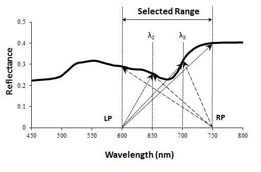
2.1. MD Applied to the Visible and NIR Range for Vegetation Research

The sensitivity analysis for the MD was conducted in the VIS to NIR regions of the spectrum through simulation of spectral reflectance of individual leaves as a function of leaf properties and canopy variables and used them to calculate the Moment Distance Index (MDI). The wavelengths of interest, between 600 and 750 nm represent more effective wavelengths for vegetation studies, notwithstanding the importance of the bands defining the peaks and trough [4] contained within the range.

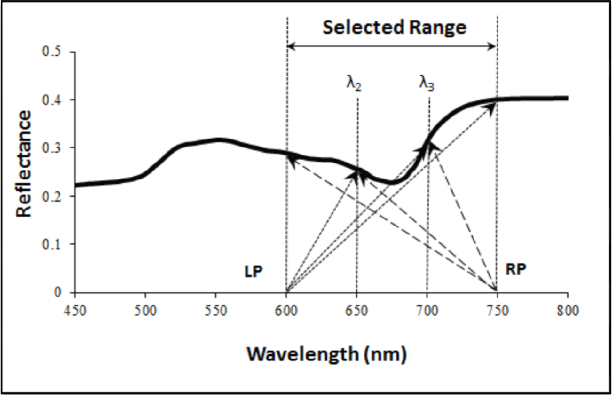
2.2. Definition and Formulation of the Moment Distance (MD)

The Moment Distance is a matrix of distances computed from two reference locations (pivots) to each spectral point within the selected range. Assume that a reflectance curve is displayed in Cartesian coordinates with the abscissa displaying the wavelength λ and the ordinate displaying the reflectance ρ (Figure 1). Let the subscript LP denote the left pivot (located in a shorter wavelength) and subscript RP denote the right pivot (located in a longer wavelength). Let λLP and λRP be the wavelength locations observed at the left and right pivots for a reflectance data, respectively, where left (right) indicates a shorter (longer) wavelength. The proposed MD approach can be described in a set of equations.
M D LP = i = λ LP λ RP ( ρ i 2 + ( i λ LP ) 2 ) 0.5
M D RP = i = λ RP λ LP ( ρ i 2 + ( λ RP i ) 2 ) 0.5
MDI = MD RP MD LP
Thus, the moment distance from the left pivot (MDLP) is the sum of the hypotenuses constructed from the left pivot to the value at successively longer wavelengths (index i from λLP to λRP); one base of the triangle is the difference from the left pivot (iλLP) along the abscissa and the other is simply the value at i (Equation (1)). Similarly, the moment distance from the right pivot (MDRP) is the sum of the hypotenuses constructed from the right pivot to the value at successively shorter wavelengths (index i from λRP to λLP); one base of the triangle is the difference from the left pivot (λRPi) along the abscissa and the other is simply the value at i (Equation (2)).
The MD Index (MDI) is an unbounded metric (Equation (3)). It increases or decreases as a nontrivial function of the number of spectral bands considered and the shape of the spectrum that spans those contiguous bands. Calculation of the MDs both from the left pivot to the right and from the right pivot to the left is necessary because the distance of a point on the curve from a reference pivot on the x-axis conveys the behavior of the curve, which is often asymmetric, from the pivot point of perspective. The more the number of points or bands considered between the pivots, the better the shape of the curve is resolved and the better the distances detect movements of trough and peak locations. The number of bands between the pivots is a function of the spectral resolution of the imaging spectrometer and the length of the selected range (i.e., full extent or subsets of the curve) being analyzed. Depending on the spectral resolution, the matrix resulting from the calculations of the MDs within a range of values could be very large. For example, a set of data having 50 bands from 400 to 900 nm could result in an initial matrix size of 51 by 51, with 2,601 entries. In hyperspectral data comprised of 1,000 bands, the matrix could contain more than one million entries. In cases with too many bands, decomposition to matrix subsets may be used to highlight specific pivot wavelength regions (PWR) [58] (e.g., 720–730 nm for vegetation red-edge; 900–980 nm for vegetation water absorption).
Figure 2 illustrates the approach. The entire Matrix 1 is a result of taking two pivots from bands λ1 to λ17. The actual matrix size is 17 by 17 with diagonals carrying the values of the reflectance equivalent to the wavelength positions. All m entries in Figure 2 represent the MD values at possible pivot pairings. Matrix 1 can be segregated into subsets with sizes that are dependent on the chosen LP and RP. Matrix 2 is a subset of Matrix 1, chosen from reference pivots λ5 and λ11. The smaller 7 by 7 matrix has five spectral bands (λ6, λ7, λ8, λ9 and λ10) in the PWR. Matrix 3 is another subset covering bands λ11 to λ16, with fours bands in another PWR. The PWR is user-selected. However, we suggest that it should be chosen according to the characterization of vegetation biophysical or biochemical property—wavelength regions that could facilitate in the detection and characterization of spectral differences, allowing separations based on the curve shapes. The same set of equations (Equations (13)) can be applied to calculate MDI for Matrices 1, 2, and 3.

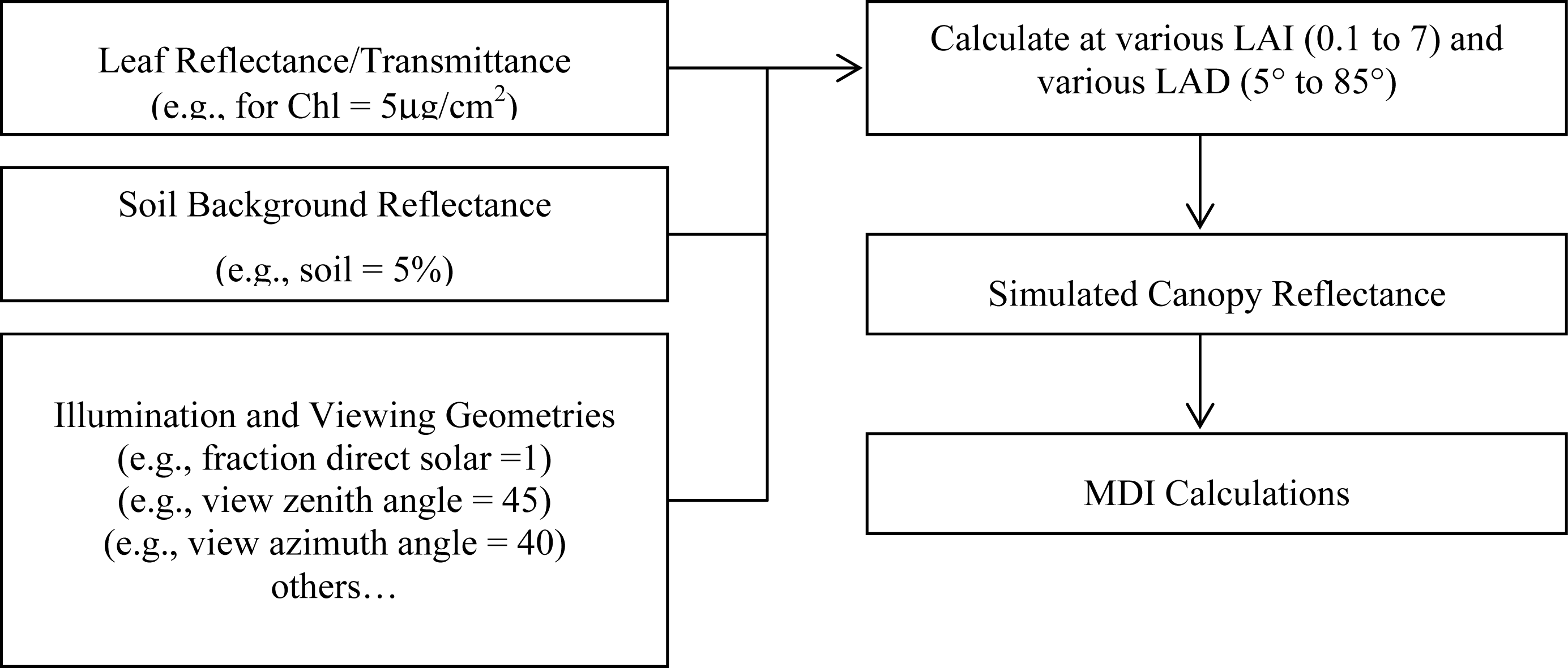
2.3. PROSPECT and SAIL Models

Physically based PROSPECT [62] and SAIL [63] models permit the extractions of major vegetation biophysical parameters and eventually provide a tool to designing algorithms for canopy biophysical and biochemical retrievals [6466]. The PROSPECT + SAIL model has been used to derive hyperspectral reflectance data and look at dynamics of vegetation indices spanning the visible and NIR regions of the spectrum [9,67]. The PROSPECT model is a simple radiative transfer model that allows the calculation of the leaf hemispherical reflectance and transmittance spectra of a leaf using only four main input parameters. Later versions of the PROSPECT have been used to evaluate the sensitivity of spectral indices to variation in soil reflectance [68].
Reflectance simulation included the range from 600 nm to 750 nm, using the PROSPECT 4 version that was developed at the USDA-ARS Hydrology and Remote Sensing Laboratory in Maryland. PROSPECT 4 combines the two absorption coefficients of total chlorophyll and total carotenoids as one [68]. The input model parameters include the leaf mesophyll structure index (n); chlorophyll content (Chl in μg/cm2); water content (wc in g/cm2), and dry matter content (dmc in g/cm2). Arbitrarily, a total of 77 leaf reflectance and transmittance spectra were simulated using the following parameters of a standard crop [62]: n = 1.83, wc = 0.0137, dmc = 0.005, and Chl ranging from 5 μg/cm2 to 80 μg/cm2 with 1 μg/cm2 increments. The output of the PROSPECT model was used as input parameters into the SAIL model.
The Scattering Arbitrary Inclined Leaves (SAIL) model is a one-dimensional, bidirectional, turbid medium radiative transfer model that simulates the reflectance and transmittance of vegetation canopies [63]. In our test, we used the SAIL model provided by the USDA Agricultural Research Service ( www.ars.usda.gov/services/software, verified 20 January 2010) that was developed in 2003 and updated in 2007. The SAIL model predicts the top-of-canopy reflectance at specific wavelengths. SAIL parameters include the controls on solar/view geometry, illumination parameters: fraction solar direct, solar declination angle, latitude, sun-view azimuth angle, view zenith angle, Leaf Angle Distribution (LAD), the Leaf Area Index (LAI), soil background reflectance and the leaf reflectance/transmittance (are importable from PROSPECT). We varied these parameters systematically to assess the sensitivity of the Moment Distance approach.
The online collection at the USGS Digital Spectral Library splib06a ( http://speclab.cr.usgs.gov; [69]) provides reflectance spectra from various types of soil and provided the range of plausible background reflectances for our simulations. We took zero as the minimum value and increased the influence to a maximum of 80% background reflectance (in steps of 5%) to cover the highest amount of soil effect to the top-of-canopy reflectance. Figure 3 shows a simple schematic diagram: from the simulations to the derivations of the MDI.

3. Results

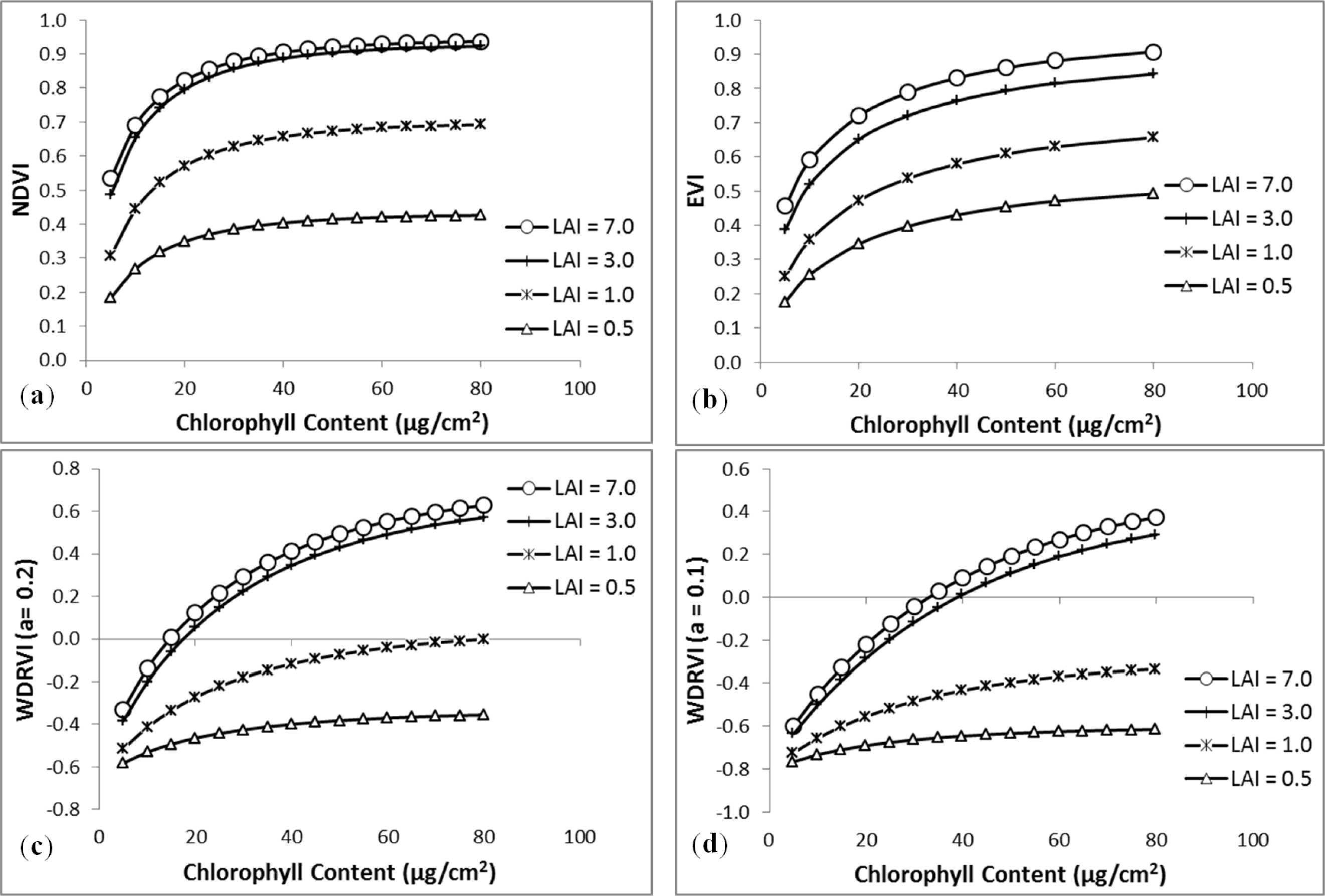
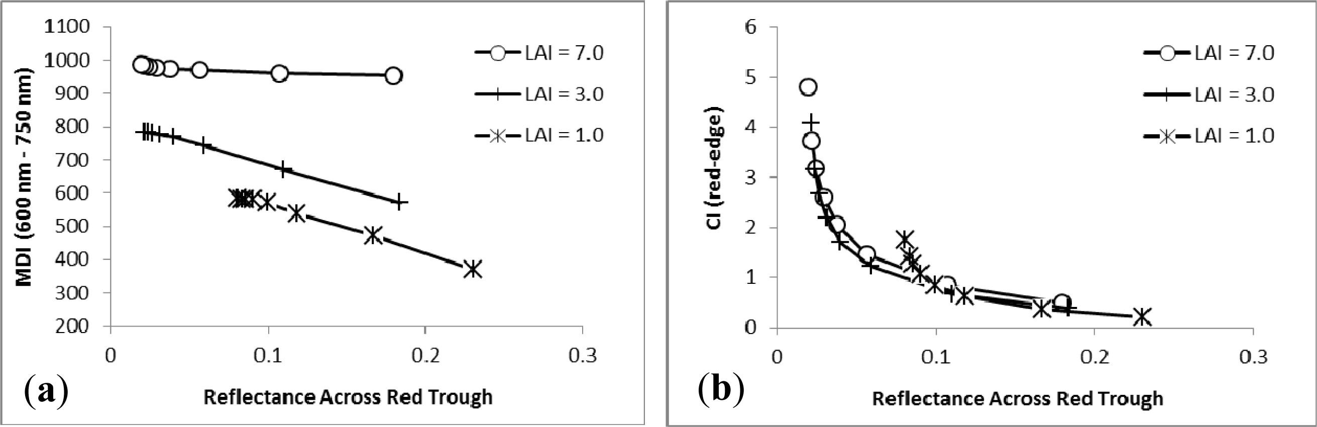
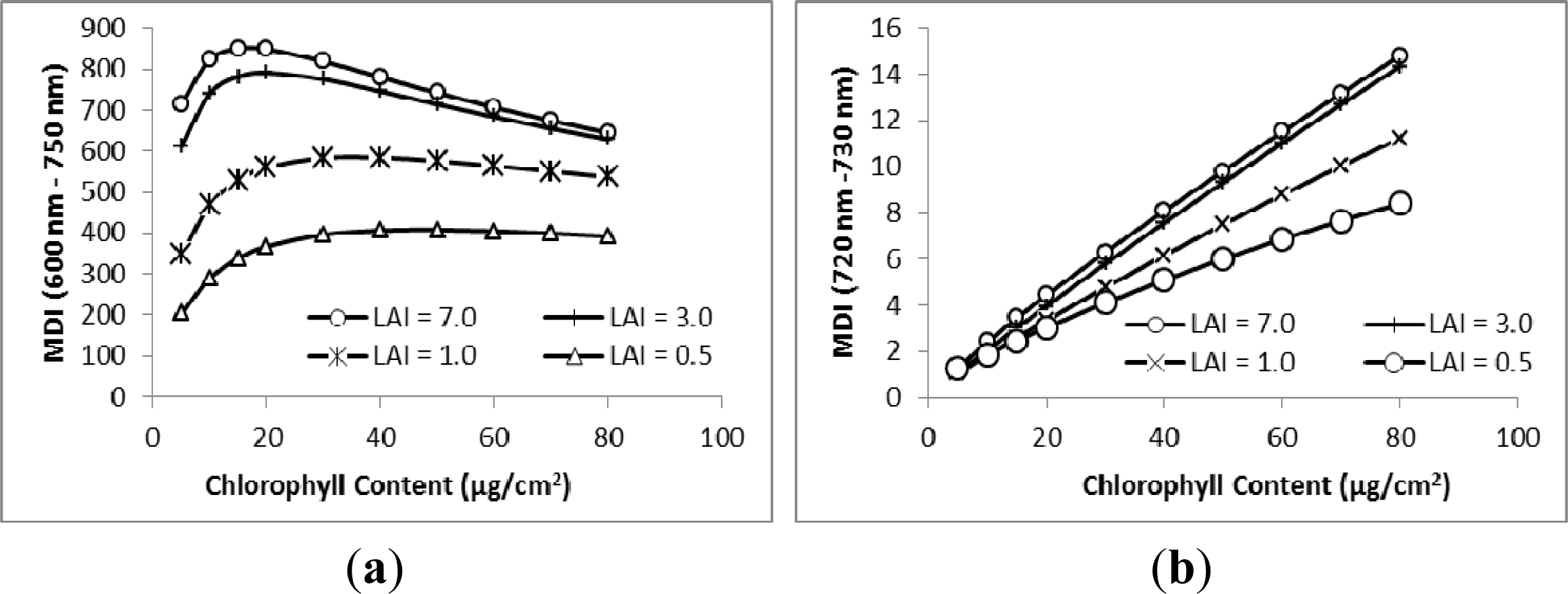
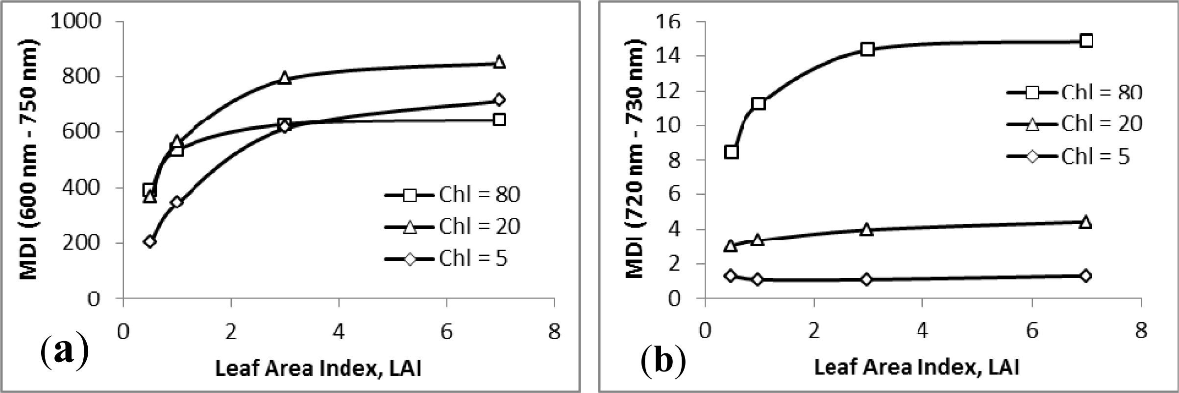
3.1. MDI on Simulated PROSECT/SAIL Reflectance Curves

The comparison between the MDI from 600 to 750 nm (MDI600–750 nm) and that from 720 to 730 nm (MDI720–730 nm) at increasing Chl is shown in Figure 4. Both show that at canopy level, small values of MDI are associated with small values of LAI. There is peaking of MDI observed in Figure 4a, at around Chl = 25 μg/cm2, before MDI decreases at increasing Chl. MDI(600–750 nm) tends to lose sensitivity at very high values of LAI and Chl. The peaking is not evident in the shorter, more specific red-edge region at 720 to 730 nm. Figure 4b shows a strong linear relationship between MDI and the Chl content at different levels of LAI. At low Chl content (e.g., Chl = 5μg/cm2), MDI values range from 1.27 to 1.31.
LAI has influence, at varying degrees, on both the MDI(600–750 nm) and MDI(720–730 nm) as shown in Figure 5a,b, respectively. The relationship between MDI and LAI is most distinct at low LAI values, with loss of sensitivity of MDI beginning at around LAI equal to 3. The trend observed between LAI and MDI when the former is below a value of about 3 may be viewed as being due to the variation in the bare soil component [70]. One interesting observation is the red-edge range (MDI720–730 nm) that tends to minimize the LAI influence (Figure 5b) even at low LAI levels.
Evident in Figure 6a,b are the differences in MDI trends in terms of the leaf inclination. Leaf angle affects the MDI at all degrees of leaf tilting for MDI(600–750 nm) (Figure 6a). MDI falls to smaller values at increasing angle. Figure 6b conveys a different story with the shorter PWR, MDI(720–730 nm), as being less affected by leaf inclination angles. Minimal effects are observed on planophile than erectophile leaves. The leaf inclination angles only began to have effects at 55° angle in low chlorophyll contents.
The PWR 600 to 750 nm is sensitive to solar zenith angle, especially at low angles (Figure 7a), with MDI leveling off at high degrees of zenith. For the 720 to 730 nm PWR, the red-edge MDI is minimally, if not affected, by zenith angle variations (Figure 7b).
Between the two diagrams in Figure 8, the fraction of direct solar irradiation (FDSI) is linearly related to the MDI(600–750 nm) (Figure 8a). The FDSI has minimal to no effects on the MDI at the red-edge feature of the spectrum (Figure 8b).
Figure 9 displays the behavior of the MDI with various percentages of soil reflectance. Soil brightness has minimal effect on the shape of the curve at range 600 to 750 nm (Figure 9a). There is significantly no effect of soil reflectance on the MDI at the strip of curve in the red-edge region. In all levels of chlorophyll content, the MDI(720–730 nm) is not associated with changes of soil reflectance (Figure 9b). The relationship between MDI and soil reflectance at varying levels of LAI is illustrated in Figure 10a,b. Both selected PWRs yielded similarities of trends—albeit MDI(720–730 nm) has a much lower LAI threshold than MDI(600–750 nm), with the latter still being sensitive at LAI greater than 3. Also, in Figure 10c,d, the proportion of soil background has clear effects on the spectral curves at varying levels of LAI.
For comparison, we used existing VIs such as the NDVI, EVI, WDRVI, CI, and CVI and checked their relationships against the chlorophyll content. We averaged spectral bands to represent NIR (750–850 nm), red (600–700 nm), blue (400–500 nm), and red-edge (690–725 nm). Figure 11 confirms the previous findings of NDVI losing sensitivity (Figure 11a) at high chlorophyll content [2]. The linear behavior of the CIred-edge and CVI against the Chl (Figure 11e,f), respectively) is similar to that in Figure 4b for MDI(720–730nm) vs. Chl. Akin to NDVI, WDRVI tended to lose sensitivity as well (Figures 11c,d), but at a much higher Chl content. EVI (Figure 11b) also lost its sensitivity at increasing Chl content. However, EVI exhibited a linear trend against Chl at a very low level of LAI (LAI = 0.5).
The result obtained when we put MDI(600–750 nm) against the magnitude of the reflectance at the trough is shown in Figure 12a. We observed indirect linear relationships, with low reflectance values relating to high MDIs. The linear trend is not manifested in CIred-edge vs. “reflectance at trough” in Figure 12b.

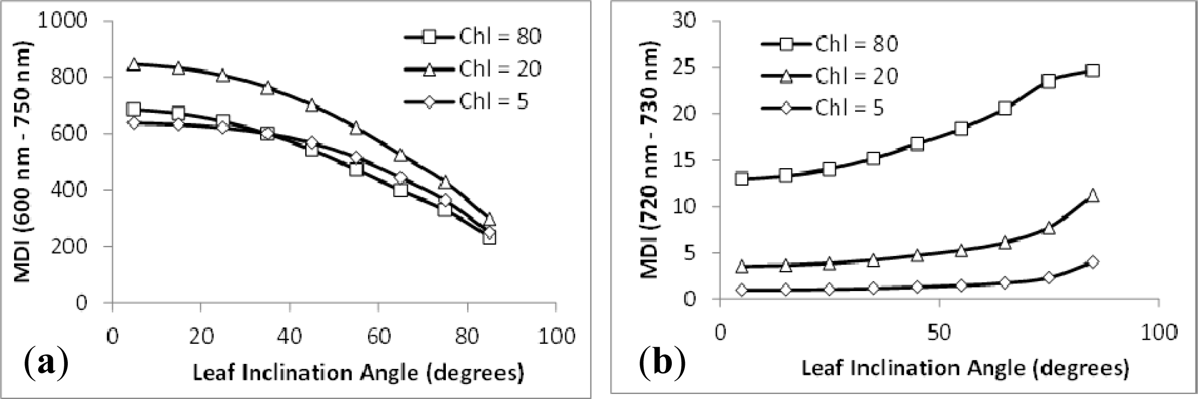
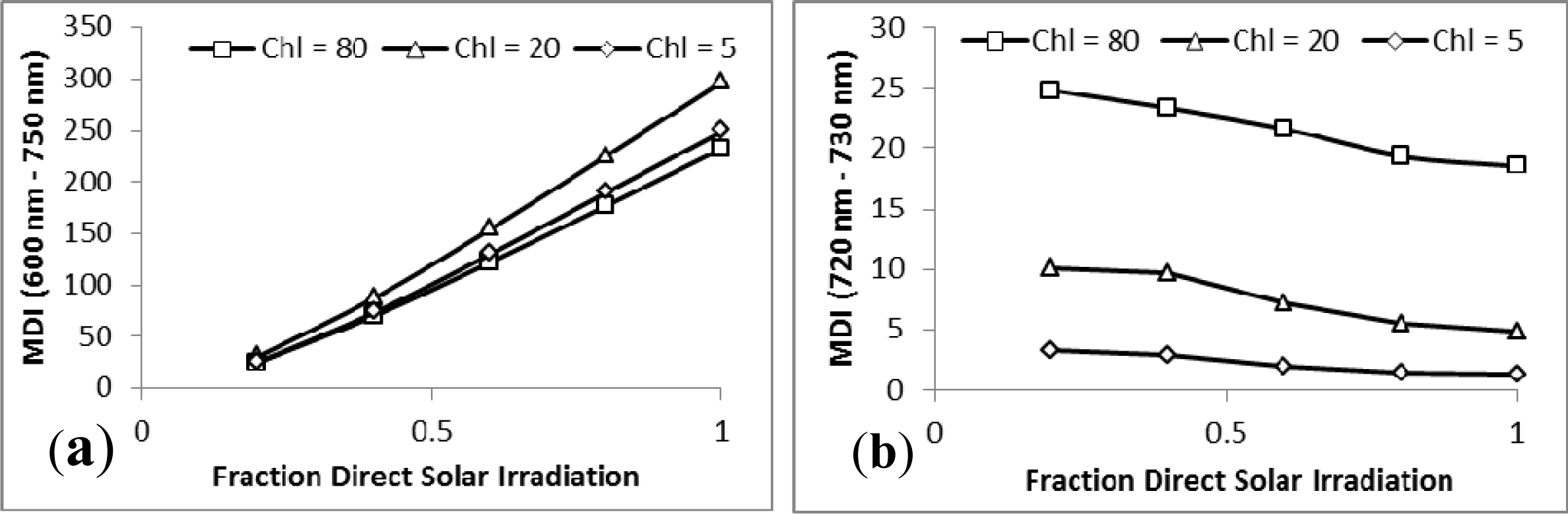
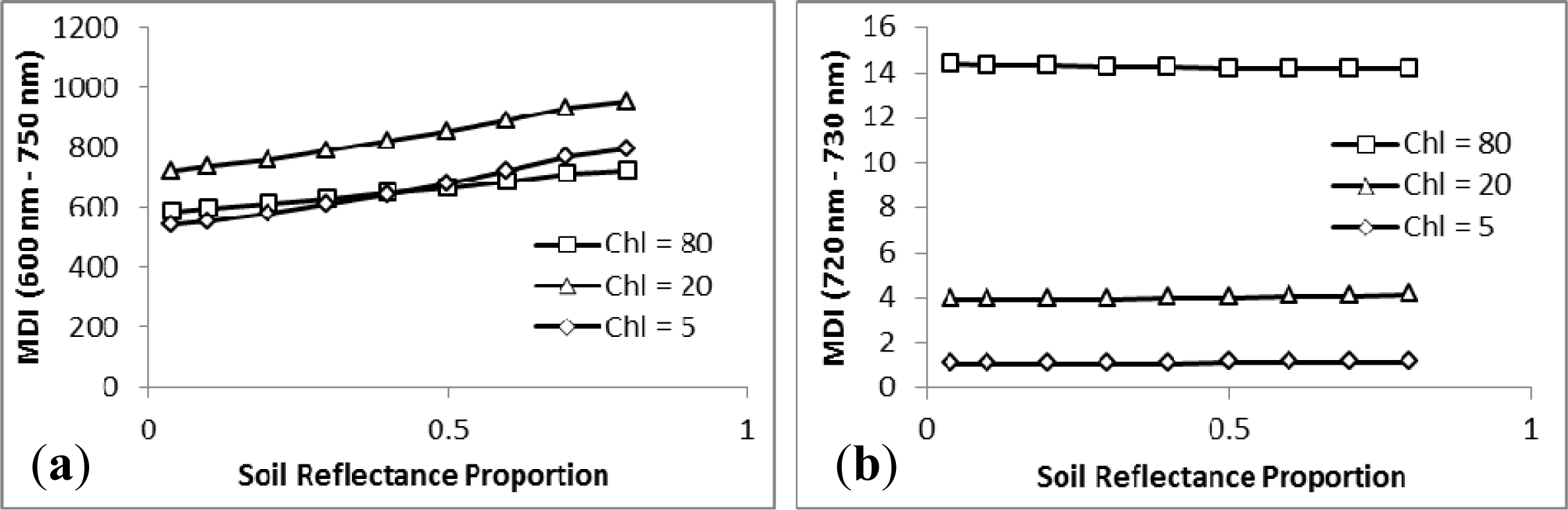
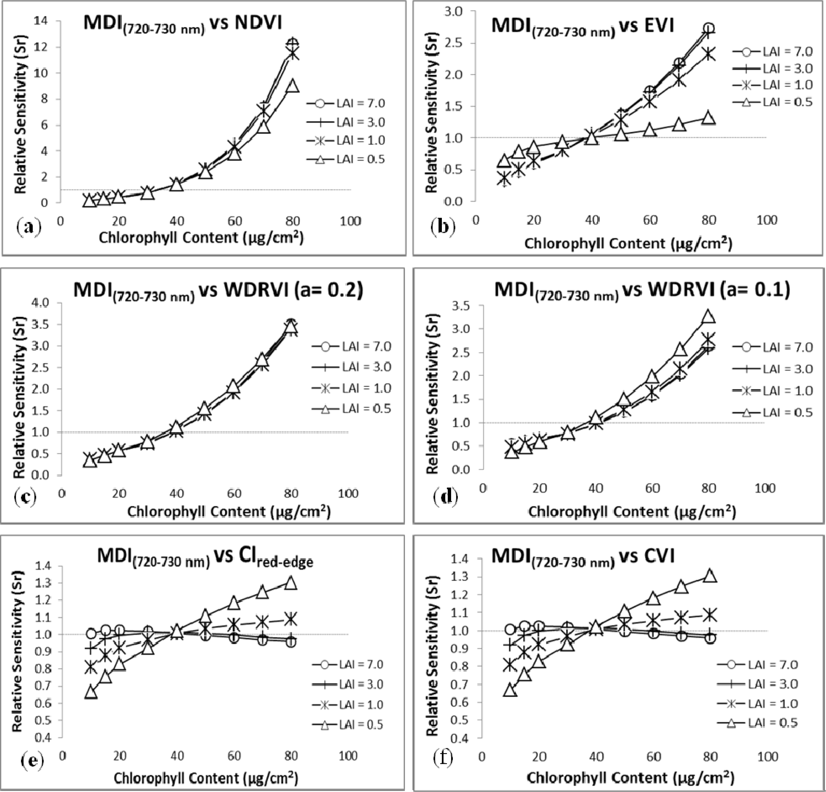
3.2. Sensitivity Analysis

The sensitivity analysis (Figure 13) complements the trends shown in Figure 11. MDI(720–730nm) is the best method in estimating Chl, especially at high Chl amounts (Chl > 40 μg/cm2). Also, MDI(720–730nm) is comparable with CVI and CIred-edge showing sensitivities of both indices to Chl interchanging at varying LAI.

4. Discussion

The MDI has three advantages compared to other existing indices. First, the MDI uses more than two or three spectral bands to infer information about vegetation properties. Its potential to utilize a number of bands at a time adds spectral information that may not be found when using reductive methods. While other studies use only a limited number of wavebands, MDI takes special attention not just on the choice of spectral bands but their positioning within an effective PWR. This leads to the second advantage: the MDI could be exploited to cover various specific PWRs as defined by pivot pairs. This characteristic enables analysis on a specialized wavelength window, e.g., red-edge region. Third, magnitude of reflectance of significant dips, such as the trough between the red and NIR bands of the spectrum, could be well detected by the MDI. A sample illustration of this observation is presented in Figure 12.
The Moment Distance metric takes advantage of the geometry of the curve. MDI detects variations of the shape or presence of significant dips and peaks due to the fixing of the two points that serve as pivots. The establishment of two pivots solidifies the MD algorithm as an approach for shape characterization by defining the structural behavior of the curve not only from a single point of perspective, but two. Movements of the key spectral landmarks, either to the shorter or longer wavelength, are manifested by change in the MD values. Equations 1 and 2, depending on the spectral resolution used, could identify the existence of changes, e.g., flattening to a rising curve, as partly illustrated by the sensitivity of MDI to the magnitude of the trough. The relation of the MDI to the changes of the spectral curve morphology is important in capturing the dynamics of the red-edge region. This paper presented results of the analysis for two sets of PWRs, the 600 to 750 nm and the much narrower spectral subset 720 to 730 nm [46]. The PWRs encompass the red and NIR and the important red-edge region [59,60,71,72] used for vegetation studies. The decomposition from full matrix to the two spectral subsets, 600 to 750 nm and 720 to 730 nm, allowed us to look at how the selected pivots define the strength of each point on the asymmetrical curve from their respective standpoint.
The high-resolution spectral data from the PROSPECT-SAIL simulations tested the sensitivity of the MDI against the vegetation properties and illumination/viewing geometries. Based on the simulation results, the MDI shows promise in detecting changes in leaf chlorophyll content at a specific PWR. While good correlations were found between the MDI and vegetation parameters at a wider LP-RP combination (600–750 nm), results show that in narrowing the PWR, a stronger and more significant relationship could be attained. Reasonable agreements depicted in the trends between MDI and other parameters (e.g., LAI, Leaf Angle Distribution) were obtained when using 600 to 750 nm. The observed trend is attributed to the entire range of variation of leaf reflectance at the 600 to 750 nm domain, where leaf reflectance increases from minimum to maximum value [73]. The MDI(600–750 nm) vs. FDSI indicated a high correlation, which could permit the MDI(600–750 nm) to be used in situations where only the spectral data is available. Figure 8 shows a strong linear trend for the MDI(600–750 nm) (larger PWR) against FDSI, something not manifested with the shorter PWR, MDI(720–730 nm). Daughtry et al. [74] also suggested a larger PWR, 500 nm to 1,100 nm.
The much narrower PWR, LP = 720 nm and RP = 730 nm, demonstrates the capability of the MDI for Chl estimation (with LAI influence minimized). MDI(720–730nm) results in a larger dynamic range against Chl than MDI(600–750 nm). In Figure 4b, increasing MDI is associated with increasing Chl, which is analogous to what is referred to as the red-shift [75], or movement of the red-edge inflection point (REIP) to longer wavelength at increasing Chl. MDI(720–730nm) detects the REIP shift when more moment distances are accumulated at the RP than the LP producing larger MDIs. RP accumulates more MD when the red trough deepens at increasing Chl producing shorter distances from the LP.
In contrast to NDVI (Figure 11a), EVI (Figure 11b), and WDRVI (Figure 11c,d)) that tend to lose sensitivity at higher chlorophyll contents, the MDI(720–730 nm) does not, as is illustrated in Figure 4. In Salas and Henebry [58], the narrow spectral range of 720 to 730 nm also performs well (r2 = 0.96) when MDI from laboratory spectra is linked to wet chemistry pigment measurements [76] such as Chl. Only the CIred-edge, which showed to be sensitive to changes in green biomass [27], and its closely related index CVI are comparable to the MDI(720–730 nm) in terms of the linear dependency to Chl content (Figure 11e,f). The CI and CVI could complement the MDI(720–730 nm) in the estimation of Chl content [58].
Since the formulation of the MD algorithm takes into account the shape of the curve, the saturation of the MDI (as shown in Figure 5 maintaining a constant value) at high LAI vindicates the unchanging shape of the curve at certain PWRs. Although red-edge indices may show the highest potential to accurately detect LAI values greater than 4 [26], our results show that it is necessary to experiment on the spectral domain for the MDI within the red-edge region. Further, the results of MDI(720–730 nm) vs. LAI suggests the possibility of looking at some other spectral PWRs for LAI estimation, or explore the sensitivities of other bands to LAI, such as the blue and green bands [77], without the MDI reaching saturation point.
There are two reasons for the reasonably good agreements of the MDI(720–730 nm) against the Chl. First, apart from the fact that the region lies in the essential vegetation spectral shift from red to NIR, the MD approach accounted for specific details of the curve at a high spectral resolution (simulating at 1 nm intervals). Second, the region is less sensitive to spectral noise caused by the soil background and by atmospheric effects [78,79]. In fact, the soil background has rather minor effects on MDI(720–730 nm). The utility of the 720–730 nm region may be compromised, however, by the effects of very low LAI and very high soil reflectance (Figure 10). Though it is shown that the influence of LAI is minimized even at low LAI values, the simulations indicate that MDI(720–730 nm) may work best for higher values of LAI, starting around LAI = 2 to 3, when the soil background reflectance becomes less significant.
Differences of the trends in the effects of the soil reflectance on the MDI in Figure 10 demonstrate the capability of the MD to detect movements of the curve shape that may be caused by soil background. Changes of the shape of the spectral curve, like the width of a trough, are shown in Figure 10c,d. Both diagrams in Figure 10a,b display the consequence of the flattening of the trough between the red and NIR as soil reflectance dominates at low LAIs.
Because most VIs lose sensitivity at very high green biomass, including NDVI, EVI, and WDRVI, it may be ideal to utilize MDI using the range 720 to 730 nm, or possibly another range within or near the red-edge region—perhaps 705 nm to 750 nm [80]—for effective Chl estimation, especially applicable at ground level where spectrometer datasets can have high spectral resolution.
The selection of pivot points is another advantage of the Moment Distance vis-à-vis other methods, as it highlights the framework as an index generation rather than a specific index. While the results show the Moment Distance being able to identify PWRs linked to vegetation properties and illumination/viewing geometries, a limitation is also exposed. The performance of the MDI is dependent on the availability of many spectral bands. For instance, the recently-launched Landsat 8 Operational Land Imager (OLI) has only nine relatively broad bands [81], which may be insufficient to detect curve changes. However, with the existence of Hyperion, a spaceborne imaging spectrometer launched in 2001 [49,67], the upcoming HyspIRI mission [50,51], airborne imaging spectrometers (e.g., AISA Eagle [82], MASTER [83], and AVIRIS [84,85]), and the advent of robust, affordable field spectrometers, fine spectral resolution datasets are increasingly available for MDI utilization.

5. Conclusions

This article has presented the definition and formulation of a new, computationally simple but powerful approach, the Moment Distance (MD), and a model-based sensitivity analysis of the Moment Distance Index (MDI) tuned to both broad and narrow spectral regions. Using the capability of the PROSPECT/SAIL to simulate a set of realistic hemispherical reflectance spectra from leaves, we have shown the potential of the Moment Distance to identify specific spectral locations linked to vegetation properties and illumination/viewing geometries. Moreover, we assessed the new algorithm against other existing indices, using subsets of wavelength regions, ensuring its sensitivity to the Chl pigment. Since the new index relies on the location of the two pivots and the number of spectral bands in between, it makes sense to explore other Moment Distance Indices defined by other PWRs not covered in this study. PWRs can be tuned in to different spectral regions for better detection of changes of shape related to pigment concentrations.
The shape of a spectral curve can be difficult to distinguish quantitatively among multiple instances of similar scenes. The MDI can be explored beyond the bands this paper has covered as its applicability to multiple bands can be perceived as more robust to fluctuations on the curve. We have seen this aspect of the MDI to be particularly important for spaceborne imaging spectrometers that may have noise or artifacts arise in particular bands, such as was experienced with Hyperion [86,87]. The Moment Distance has the potential to spread retrieval risk across several bands while retaining sensitivity.
In an attempt to define the shape of the curve and its benefits to vegetation spectral property estimation, we developed the algorithm with the assumption that specific spectral PWRs and the wavebands contained in it could define the curve and its movement. We conclude in our test that the MD approach has succeeded in at least three ways.
First, the approach allows the use of the reflectance data without having to go through any transformation method. It does not limit itself from two to three bands to infer spectral information; rather, it utilizes more bands through a simple algorithm. The method of considering more bands may be seen as an impediment to a swifter analysis. Nonetheless, this should not be considered a limitation, but an essential feature of the approach for analyzing shape and deriving additional information from the curve. Also, simplicity in the analysis is one of the highlights of the MD. In the development of the algorithm, the Pythagorean Theorem is introduced as its base concept, all for ease in the computation of the moment distances. The introduction of the PWR showed the possibility of looking at and analyzing hyperspectral dataset in a different way.
Second, the choice of the red and NIR bands for our testing not only confirms the importance of the red-edge region, as many previous studies have suggested, but also shows the MDI as a comparable, if not better, index for photosynthetic pigment estimation. For instance, the MDI performs well in our investigations against the Chl. In fact, in the sensitivity analysis, MDI is the best method in estimating Chl, especially at high Chl amounts. Also, contrasting trends found in both PWRs—720 to 730 nm and 600 to 750 nm—open doors for MD exploration over a wide range of spectral domains and endless decomposition of the curve—varying range locations, number of bands, and relating to various vegetation properties or parameters.
Third, MD demonstrates the possibility of looking at movements in spectral reflectance by constricting the shape within pivots. MD is sensitive to changes in the asymmetrical shape of the curve as shown in our results in Figure 10 when the spectral curves vary with differing proportion of soil background at various levels of LAI. The MDI responds to changes of shape in the spectral curve through the difference between the MD from the left pivot to the right from the MD calculated from the right pivot to the left. Such changes in the shape of a spectrum are difficult to observe using band ratios that emphasize differences in magnitude of just a few bands.
One of the important prospects for positions of our results is in the simulation of sensor bands. For example, spectral bands from imaging spectrometers, both airborne (e.g., AISA Eagle, AVIRIS, MASTER) and spaceborne (e.g., EO-1 Hyperion and HyspIRI), can be mimicked using the exact band centers in the PROSPECT/SAIL simulation. Utilizing various PWRs, we can look at relationships of the new algorithm against vegetation parameters, especially when enhancing the spectral resolution by adding new bands in between, or deleting existing ones, or averaging the bands. In addition, a study can be done to evaluate whether the results achieved using the simulated hyperspectral spectra will hold true with sensors with multispectral bands, such as the Landsat sensors (TM/ETM+/OLI).
Finally, our experimental results indicate that the new MD approach can specifically narrow pre-identified and wider wavelength regions, such as the red and NIR, that are important for vegetation studies by exploiting the concept of PWR. We hope that what we presented here could lead to improved hyperspectral analysis through acquiring a better understanding of the curve structure and gathering more information latent in the shape of the reflectance curve. Though our findings here are limited to shapes of spectral reflectance, we are certain that the method can be applied beneficially to other types of curves.

Acknowledgments

The research is supported in part by a GSCE graduate research fellowship and by NASA project NNX09AK23G.

Conflicts of Interest

The authors declare no conflict of interest.

References

  1. Chen, J.M.; Cihlar, J. Retrieving leaf area index of boreal conifer forests using Landsat TM images. Remote Sens. Environ 1996, 55, 153–162. [Google Scholar]
  2. Gitelson, A.A.; Merzlyak, M.N. Quantitative estimation of chlorophyll-a using reflectance spectra: Experiments with autumn chestnut and maple leaves. J. Photochem. Photobiol. B: Biol 1994, 22, 247–252. [Google Scholar]
  3. Skianis, G.; Vaiopoulos, D.; Nikolakopoulos, K. A Comparative Study of the Performance of the NDVI, the TVI and the SAVI Vegetation Indices over Burnt Areas, Using Probability Theory and Spatial Analysis Techniques. Proceedings of the 6th International Workshop of the EARSeL Special Interest Group on Forest Fires, Thessaloniki, Greece, 27–29 September 2007.
  4. Tucker, C.J. Red and photographic infrared linear combinations for monitoring vegetation. Remote Sens. Environ 1979, 8, 127–150. [Google Scholar]
  5. Clevers, J.G.P.W. Application of a vegetation index in correcting the infrared reflectance for soil background. Int. Arch. Photogramm. Remote Sens. Spat. Inf. Sci 1988, 16, 221–226. [Google Scholar]
  6. Gitelson, A.A. Wide Dynamic range vegetation index for remote quantification of biophysical characteristics of vegetation. J. Plant Physiol 2004, 161, 165–173. [Google Scholar]
  7. Steele, M.R.; Gitelson, A.A.; Rundquist, D.C. Nondestructive estimation of anthocyanin content in Grapevine leaves. Am. J. Enol. Vitic 2009, 60, 87–92. [Google Scholar]
  8. Salas, E.A.L.; Henebry, G.M. Area between peaks feature in the derivative reflectance curve as a sensitive indicator of change in chlorophyll concentration. GISci. Remote Sens 2009, 46, 315–328. [Google Scholar]
  9. Broge, N.H.; Leblanc, E. Comparing prediction power and stability of broadband and hyperspectral vegetation indices for estimation of green leaf area index and canopy chlorophyll density. Remote Sens. Environ 2001, 76, 156–172. [Google Scholar]
  10. Okin, G.S. The contribution of brown vegetation to vegetation dynamics. Ecology 2010, 91, 743–755. [Google Scholar]
  11. Pettorelli, N.; Vik, J.O.; Mysterud, A.; Gaillard, J.-M.; Tucker, C.J.; Stenseth, N.C. Using the satellite-derived NDVI to assess ecological responses to environmental change. Trends Ecol. Evol 2005, 20, 503–510. [Google Scholar]
  12. Townshend, J.R.G.; Justice, C.O. Analysis of the dynamics of African vegetation using the normalized difference vegetation index. Int. J. Remote Sens 1986, 7, 1435–1445. [Google Scholar]
  13. Viña, A.; Henebry, G.M.; Gitelson, A.A. Satellite monitoring of vegetation dynamics: Sensitivity enhancement by the Wide Dynamic Range Vegetation Index. Geophys. Res. Lett 2004. [Google Scholar] [CrossRef]
  14. Hurcom, S.J.; Harrison, A.R. The NDVI and spectral decomposition for semi-arid vegetation abundance estimation. Int. J. Remote Sens 1998, 19, 3109–3125. [Google Scholar]
  15. Simms, E.L.; Ward, H. Multisensor NDVI-based monitoring of the Tundra-Taiga interface (Mealy Mountains, Labrador, Canada). Remote Sens 2013, 5, 1066–1090. [Google Scholar]
  16. Rouse, J.W., Jr.; Haas, R.H.; Schell, J.A.; Deering, D.W. Monitoring Vegetation System in the Great Plains with ERTS. Proceedings of the Third Earth Resources Technology Satellite-1 Symposium, Greenbelt, MD, USA, 10–14 December 1974; pp. 309–317.
  17. Haboudane, D.; Miller, J.R.; Pattey, E.; Zarco-Tejada, P.J.; Strachan, I.B. Hyperspectral vegetation indices and novel algorithms for predicting green LAI of crop canopies: Modeling and validation in the context of precision agriculture. Remote Sens. Environ 2004, 90, 337–352. [Google Scholar]
  18. Myneni, R.B.; Hall, F.G.; Sellers, P.J.; Marshak, A.L. The interpretation of spectral vegetation indexes. IEEE Trans. Geosci. Remote Sens 1995, 33, 481–486. [Google Scholar]
  19. Zhao, X.; Tan, K.; Zhao, S.; Fang, J. Changing climate affects vegetation growth in the arid region of the northwestern China. J. Arid Environ 2011, 75, 946–952. [Google Scholar]
  20. Rondeaux, G.; Steven, M.; Baret, F. Optimization of soil-adjusted vegetation indices. Remote Sens. Environ 1996, 55, 95–107. [Google Scholar]
  21. Elvidge, C.D.; Chen, Z. Comparison of broad-band and narrow-band red and near-infrared vegetation indices. Remote Sens. Environ 1995, 54, 38–48. [Google Scholar]
  22. Jordan, C.F. Derivation of leaf area index from quality of light on the forest floor. Ecology 1969, 50, 663–666. [Google Scholar]
  23. Pearson, R.L.; Miller, L.D. Remote Mapping of Standing Crop Biomass for Estimation of the Productivity of the Short-Grass Prairie. Proceedings of the Eighth International Symposium on Remote Sensing of Environment, Pawnee National Grasslands, Colorado, Ann Arbor, MI, USA, 2–6 October 1972; pp. 357–1381.
  24. Baret, F.; Guyot, G. Potentials and limits of vegetation indices for LAI and APAR assessment. Remote Sens. Environ 1991, 35, 161–173. [Google Scholar]
  25. Gitelson, A.A.; Viña, A.; Arkebauer, T.J.; Rundquist, D.C.; Keydan, G.; Leavitt, B. Remote estimation of leaf area index and green leaf biomass in maize canopies. Geophys. Res. Lett 2003. [Google Scholar] [CrossRef]
  26. Brantley, S.T.; Zinnert, J.C.; Young, D.R. Application of hyperspectral vegetation indices to detect variations in high leaf area index temperate shrub thicket canopies. Remote Sens. Environ 2011, 115, 514–523. [Google Scholar]
  27. Viña, A. Evaluating vegetation indices for assessing productivity along a tropical rain forest chronosequence in Western Amazonia. Isr. J. Plant Sci 2012, 60, 123–133. [Google Scholar]
  28. Viña, A.; Gitelson, A.A. New developments in the remote estimation of the fraction of absorbed photosynthetically active radiation in crops. Geophys. Res. Lett 2005. [Google Scholar] [CrossRef]
  29. Aguilar-Amuchastegui, N.; Henebry, G.M. Characterizing tropical forest spatio-temporal heterogeneity using the Wide Dynamic Range Vegetation Index (WDRVI). Int. J. Remote Sens 2008, 29, 7285–7291. [Google Scholar]
  30. Aguilar-Amuchastegui, N.; Henebry, G.M. Monitoring sustainability in tropical forests: How changes in canopy spatial pattern can indicate forest stands for biodiversity surveys. IEEE Geosci. Remote Sens. Lett 2006, 3, 329–333. [Google Scholar]
  31. Gitelson, A.A. Remote estimation of crop fractional vegetation cover: The use of noise equivalent as an indicator of performance of vegetation indices. Int. J. Remote Sens 2013, 34, 6054–6066. [Google Scholar]
  32. Deering, D.W.; Rouse, J.W.; Haas, R.H.; Schell, J.A. Measuring Forage Production of Grazing Units from Landsat MSS Data. Processings of the 10th International Symposium on Remote Sensing of Environment, Ann Arbor, MI, USA, October 1975; pp. 1169–1178.
  33. Gilabert, M.A.; González-Piqueras, J.; Garcýìa-Haro, F.J.; Meliá, J. A generalized soil-adjusted vegetation index. Remote Sens. Environ 2002, 82, 303–310. [Google Scholar]
  34. Baret, F.; Jacquemoud, S.; Hanocq, J.F. About the soil line concept in remote sensing. Adv. Sp. Res 1993, 13, 281–284. [Google Scholar]
  35. Richardson, A.J.; Wiegand, C.L. Distinguishing vegetation from soil background information. Photogramm. Eng. Remote Sens 1977, 43, 1541–1552. [Google Scholar]
  36. Qi, J.; Chehbouni, A.; Huete, A.R.; Kerr, Y.H.; Sorooshian, S. A modified soil adjusted vegetation index. Remote Sens. Environ 1994, 48, 119–126. [Google Scholar]
  37. Perry, J.C.R.; Lautenschlager, L.F. Functional equivalence of spectral vegetation indices. Remote Sens. Environ 1984, 14, 169–182. [Google Scholar]
  38. Kauth, R.J.; Thomas, G.S. The Tasseled Cap—A Graphic Description of the Spectral-Temporal Development of Agricultural Crops as Seen in Landsat. Proceedings of the Symposium on Machine Processing of Remotely Sensed Data, West Lafayette, IN, USA, 29 June–1 July 1976; pp. 41–51.
  39. Crist, E.P.; Cicone, R.C. A physically-based transformation of thematic mapper data: The TM Tassed Cap. IEEE. Trans. Geosci. Remote Sens 1984, 22, 256–263. [Google Scholar]
  40. Gitelson, A.A.; Stark, R.; Grits, U.; Rundquist, D.; Kaufman, Y.; Derry, D. Vegetation and soil lines in visible spectral space: A concept and technique for remote estimation of vegetation fraction. Int. J. Remote Sens 2002, 23, 2537–2562. [Google Scholar]
  41. Huete, A.R. A soil-adjusted vegetation index (SAVI). Remote Sens. Environ 1988, 25, 295–309. [Google Scholar]
  42. Baret, F.; Guyot, G.; Major, D.J. TSAVI: A Vegetation Index which Minimizes Soil Brightness Effects on LAI and APAR Estimation. Proceedings of the 12th Canadian Symposium on Remote Sensing, Vancouver, BC, Canada, 10–14 July 1989; pp. 1355–1358.
  43. Major, D.J.; Baret, F.; Guyot, G. A ratio vegetation index adjusted for soil brightness. Int. J. Remote Sens 1990, 11, 727–740. [Google Scholar]
  44. Bannari, A.; Huete, A.R.; Morin, D.; Zagolski, F. Effects of soil colour and brightness on vegetation index. Int. J. Remote Sens 1996, 17, 1885–1906. [Google Scholar]
  45. Liu, H.Q.; Huete, A.R. A feedback based modification of the NDVI to minimize canopy background and atmospheric noise. IEEE Trans. Geosci. Remote Sens 1995, 33, 457–465. [Google Scholar]
  46. Gitelson, A.A.; Keydan, G.P.; Merzlyak, M.N. Three-band model for noninvasive estimation of chlorophyll, carotenoids, and anthocyanin contents in higher plant leaves. Geophys. Res. Lett 2006. [Google Scholar] [CrossRef]
  47. Nguy-Robertson, A.; Gitelson, A.; Peng, Y.; Vina, A.; Arkebauer, T.; Rundquist, D. Green leaf area index estimation in maize and soybean: Combining vegetation indices to achieve maximal sensitivity. Agron. J 2012, 104, 1336–1347. [Google Scholar]
  48. Yoshioka, H.; Miura, T.; Demattê, J.A.M.; Batchily, K.; Huete, A.R. Derivation of soil line influence on two-band vegetation indices and vegetation isolines. Remote Sens 2009, 1, 842–857. [Google Scholar]
  49. Pearlman, J.S.; Barry, P.S.; Segal, C.C.; Shepanski, J.; Beiso, D.; Carman, S.L. Hyperion, a space-based imaging spectrometer. IEEE Trans. Geosci. Remote Sens 2003, 41, 1160–1173. [Google Scholar]
  50. Kruse, F.A.; Taranik, J.V.; Coolbaugh, M.; Michaels, J.; Littlefield, E.F.; Calvin, W.M.; Martini, B.A. Effect of reduced spatial resolution on mineral mapping using imaging spectrometry—Examples using Hyperspectral Infrared Imager (HyspIRI)-simulated data. Remote Sens 2011, 3, 1584–1602. [Google Scholar]
  51. Mariotto, I.; Thenkabail, P.S.; Huete, A. R.; Slonecker, E.T.; Platonov, A. Hyperspectral vs. multispectral crop-productivity modeling and type discrimination for the HyspIRI mission. Remote Sens. Environ 2013, 139, 291–305. [Google Scholar]
  52. Wang, L.; Hunt, E.R.; Qu, J.J.; Hao, X.; Daughtry, C.S.T. Towards estimation of canopy foliar biomass with spectral reflectance measurements. Remote Sens. Environ 2011, 115, 836–840. [Google Scholar]
  53. Roberts, D.A.; Roth, K.L.; Perroy, R.L. Hyperspectral Vegetation Indices. In Hyperspectral Remote Sensing of Vegetation; Thenkabail, P.S., Lyon, J.G., Huete, A.R., Eds.; CRC Press: Boca Raton, FL, USA, 2012. [Google Scholar]
  54. Cho, M.A.; Skidmore, A.K.; Atzberger, C. Towards red-edge positions less sensitive to canopy biophysical parameters for leaf chlorophyll estimation using properties optique spectrales des feuilles (PROSPECT) and scattering by arbitrarily inclined leaves (SAILH) simulated data. Int. J. Remote Sens 2008, 29, 2241–2255. [Google Scholar]
  55. Filella, I.; Peñuelas, J. The red edge position and shape as indicators of plant chlorophyll content, biomass and hydric status. Int. J. Remote Sens 1994, 15, 1459–1470. [Google Scholar]
  56. Banskota, A.; Wynne, R.H.; Thomas, V.A.; Serbin, S.P.; Kayastha, N.; Gastellu-Etchegorry, J.P.; Townsend, P.A. Investigating the utility of wavelet transforms for inverting a 3-D radiative transfer model using hyperspectral data to retrieve forest LAI. Remote Sens 2013, 5, 2639–2659. [Google Scholar]
  57. Gitelson, A.A.; Merzlyak, M.N. Signature analysis of leaf reflectance spectra: Algorithm development for remote sensing of chlorophyll. J. Plant Physiol 1996, 148, 494–500. [Google Scholar]
  58. Salas, E.A.L.; Henebry, G.M. Separability of maize and soybean in the spectral regions of chlorophyll and carotenoids using the Moment Distance Index. Isr. J. Plant Sci 2012, 60, 65–76. [Google Scholar]
  59. Horler, D.N.H.; Dockray, M.; Barber, J. The red-edge of plant leaf reflectance. Int. J. Remote Sens 1983, 4, 273–288. [Google Scholar]
  60. Liao, Q.; Wang, J.; Yang, G.; Zhang, D.; Li, H.; Fu, Y.; Li, Z. Comparison of spectral indices and wavelet transform for estimating chlorophyll content of maize from hyperspectral reflectance. J. App. Remote Sens 2013, 7. [Google Scholar] [CrossRef]
  61. Gitelson, A.A. Nondestructive Estimation of Foliar Pigment (Chlorophylls, Carotenoids, and Anthocyanins) Contents: Evaluating a Semianalytical Three-Band Model. In Hyperspectral Remote Sensing of Vegetation; Thenkabail, P.S., Lyon, J.G., Huete, A.R., Eds.; CRC Press: Boca Raton, FL, USA, 2011. [Google Scholar]
  62. Jacquemoud, S.; Baret, F. PROSPECT: A model of leaf optical properties spectra. Remote Sens. Environ 1990, 34, 75–91. [Google Scholar]
  63. Verhoef, W. Light scattering by leaf layers with application to canopy reflectance modeling: The SAIL model. Remote Sens. Environ 1984, 16, 125–141. [Google Scholar]
  64. Atzberger, C.; Darvishzadeh, R.; Schlerf, M.; Le Maire, G. Suitability and adaptation of PROSAIL radiative transfer model for hyperspectral grassland studies. Remote Sens. Lett 2013, 4, 55–64. [Google Scholar]
  65. Uto, K.; Kosugi, Y. Leaf parameter estimation based on leaf scale hyperspectral imagery. IEEE J. Sel. Top. Appl. Earth Obs. Remote Sens 2013, 6, 699–707. [Google Scholar]
  66. Croft, H.; Chen, J.M.; Zhang, Y.; Simic, A. Modelling Leaf Chlorophyll Content in Broadleaf and Needle Leaf Canopies from Ground, CASI, Landsat TM 5 and MERIS Reflectance Data. Remote Sens. Environ 2013, 133, 128–140. [Google Scholar]
  67. Navarro-Cerrillo, R.M.; Trujillo, J.; Sanchez de la Orden, M.; Hernandez-Clemente, R. Hyperspectral and multispectral satellite sensors for mapping chlorophyll content in a Mediterranean pinus sylvestris L. plantation. Int. J. Appl. Earth Obs. Geoinf 2014, 26, 88–96. [Google Scholar]
  68. Feret, J.-B.; François, C.; Asner, G.P.; Gitelson, A.A.; Martin, R.E.; Bidel, L.P.R.; Ustin, S.L.; le Maire, G.; Jacquemoud, S. PROSPECT-4 and 5: Advances in the leaf optical properties model separating photosynthetic pigments. Remote Sens. Environ 2008, 112, 3030–3043. [Google Scholar]
  69. Clark, R.N.; Swayze, G.A.; Wise, R.; Livo, E.; Hoefen, T.; Kokaly, R.; Sutley, S.J. USGS Digital Spectral Library Splib06a. Available online: http://speclab.cr.usgs.gov/spectral.lib06 (accessed on 10 March 2010).
  70. Carlson, T.N.; Ripley, D.A. On the relation between NDVI, fractional vegetation cover, and leaf area index. Remote Sens. Environ 1997, 62, 241–252. [Google Scholar]
  71. Ahern, F.J. The effects of bark beetle stress on the foliar spectral reflectance of Lodgepole Pine. Int. J. Remote Sens 1988, 9, 1451–1468. [Google Scholar]
  72. Curran, P.J.; Dungan, J.L.; Gholz, H.L. Exploring the relationship between reflectance red edge and chlorophyll content in slash pine. Tree Physiol 1991, 7, 33–48. [Google Scholar]
  73. Baret, F.; Vanderbilt, V.C.; Steven, M.D.; Jacquemoud, S. Use of spectral analogy to evaluate canopy reflectance sensitivity to leaf optical properties. Remote Sens. Environ 1994, 48, 253–260. [Google Scholar]
  74. Daughtry, C.S.T.; Gallo, K.P.; Bauer, M.E. Spectral estimates of solar radiation intercepted by corn canopies. Agron. J 1983, 75, 527–531. [Google Scholar]
  75. Clevers, J.G.P.W.; Kooistra, L.; Salas, E.A.L. Study of heavy metal contamination in river floodplains using the red-edge position in spectroscopic data. Int. J. Remote Sens 2004, 25, 3883–3895. [Google Scholar]
  76. Gitelson, A.A.; Vina, A.; Rundquist, D.C.; Ciganda, V.; Arkebauer, T.J. Remote estimation of canopy chlorophyll content in crops. Geophys. Res. Lett 2005. [Google Scholar] [CrossRef]
  77. Wang, F.-M.; Huang, J.-F; Tang, Y.-L; Wang, X.-Z. New vegetation index and its application in estimating leaf area index of rice. Rice Sci 2007, 14, 195–203. [Google Scholar]
  78. Demetriades-Shah, T.H.; Steven, M.D.; Clark, J.A. High resolution derivative spectra in remote sensing. Remote Sens. Environ 1990, 33, 55–64. [Google Scholar]
  79. Baret, F.; Jacquemoud, S.; Guyot, G.; Leprieur, C. Modeled analysis of the biophysical nature of spectral shifts and comparison with information content of broad bands. Remote Sens. Environ 1992, 41, 133–142. [Google Scholar]
  80. Wu, C.; Niu, Z.; Tang, Q.; Huang, W. Estimating chlorophyll content from hyperspectral vegetation indices: Modeling and validation. Agric. For. Meteorol 2008, 148, 1230–1241. [Google Scholar]
  81. Irons, J.R.; Dwyer, J.L.; Barsi, J.A. The next Landsat satellite: The Landsat Data Continuity Mission. Remote Sens. Environ 2012, 122, 11–21. [Google Scholar]
  82. Mishra, D.R.; Narumalani, S.; Rundquist, D.; Lawson, M.; Perk, R. Enhancing the detection and classification of coral reef and associated benthic habitats: A hyperspectral remote sensing approach. J. Geophys. Res 2007, 112. [Google Scholar] [CrossRef]
  83. Hook, S.J.; Myers, J.E.J.; Thome, K.J.; Fitzgerald, M.; Kahle, A.B. The MODIS/ASTER airborne simulator (MASTER)—A new instrument for earth science studies. Remote Sens. Environ 2001, 76, 93–102. [Google Scholar]
  84. Miller, J.R.; Freemantle, J.R.; Belanger, M.J.; Elvidge, C.D.; Boyer, M.G. Potential for Determination of Leaf Chlorophyll Content Using AVIRIS. Proceedings of the Second Airborne Visible/Infrared Imaging Spectrometer (AVIRIS) Workshop, Pasadena, CA, USA, 4–5 June 1990; pp. 72–77.
  85. Green, R.O.; Eastwood, M.L.; Sarture, C.M.; Chrien, T.G.; Aronsson, M.; Chippendale, B.J.; Faust, J.A.; Pavri, B.E.; Chovit, C.J.; Solis, M.; et al. Imaging spectroscopy and the Airborne Visible/Infrared Imaging Spectrometer (AVIRIS). Remote Sens. Environ 1998, 65, 227–248. [Google Scholar]
  86. Liao, L.; Jarecke, P.; Gleichauf, D.; Hedman, T. Performance characterization of the Hyperion imaging spectrometer instrument. Proc. SPIE 2000, 4135. [Google Scholar] [CrossRef]
  87. Chen, W.; Henebry, G.M. Spatio-spectral heterogeneity analysis using EO-1 Hyperion imagery. Comput. Geosci 2010, 36, 167–170. [Google Scholar]
Figure 1. MD Index schematic diagram for spectral reflectance curve. Note that the number of points between LP and RP pivots can vary depending on the spectral resolution and the width of the selected range.
Remotesensing 06 00020f1
Figure 2. Components of the initial MD matrix and its subsets: Wavelength component, λ, in the first column; reflectance, R, on the diagonal; other entries represent individual moment distances, m, from reference points.
Remotesensing 06 00020f2
Figure 3. Example schematic diagram of how parameters are varied in the simulation. The process can be repeated at other values of Chl, background reflectance, and illumination and viewing geometries to produce simulated canopy reflectance.
Remotesensing 06 00020f3
Figure 4. Relationships of MDI against Chl for PWR (a) 600 to 750 nm and (b) 720 to 730 nm. Take note of the linearity shown by the spectral range 720 to 730 nm against Chl, suggesting that it may be a better range for Chl estimation.
Remotesensing 06 00020f4
Figure 5. Relationships of MDI against LAI for PWR (a) 600 to 750 nm and (b) 720 to 730 nm. Note how the MDI computed from 600 to 750 nm PWR loses sensitivity around LAI = 3. The range 720 to 730 nm, however, tends to minimize the LAI influence.
Remotesensing 06 00020f5
Figure 6. Relationships of MDI against leaf inclination angle for PWR (a) 600 to 750 nm and (b) 720 to 730 nm. The MDI from 600 to 750 nm range is sensitive to leaf inclination at almost all angles. Leaf angle has minimal effects on MDI(720–730 nm).
Remotesensing 06 00020f6
Figure 7. Relationships of MDI against solar zenith angle for PWR (a) 600 to 750 nm and (b) 720 to 730 nm. Note that the MDI from 720 to 730 nm is minimally affected by solar zenith angle.
Remotesensing 06 00020f7
Figure 8. Relationships of MDI against fraction of direct solar irradiation for PWR (a) 600 to 750 nm and (b) 720 to 730 nm. The larger PWR is more sensitive to FDSI.
Remotesensing 06 00020f8
Figure 9. Relationships of MDI against soil background reflectance for PWR (a) 600 to 750 nm and (b) 720 to 730 nm. Very minimal background effect has been observed using the shorter range.
Remotesensing 06 00020f9
Figure 10. Relationships of MDI against soil background reflectance in varying levels of LAI for PWR (a) 600 to 750 nm and (b) 720 to 730 nm. No background effect has been observed using the red-edge spectral range, especially for LAI equal to 2 and higher. (c,d) spectral curves are affected by proportions of soil background at varying levels of LAI.
Remotesensing 06 00020f10
Figure 11. Chl content vs. (a) NDVI (b) EVI (c) WDRVI with a = 0.2 (d) WDRVI with a = 0.1 (e) CIred-edge (f) CVI. Note how the NDVI loses sensitivity at smaller quantity of Chl content. Also, CIred-edge and CVI show clear linear trends comparable with MDI(720–730nm).
Remotesensing 06 00020f11aRemotesensing 06 00020f11b
Figure 12. Magnitude of the reflectance across the red trough falling between the 600 nm to 750 nm against (a) MDI(600–750 nm) (b) CIred-edge. CIred-edge loses sensitivity at higher trough reflectance.
Remotesensing 06 00020f12
Figure 13. Relative sensitivity (Sr) of MDI(720–730nm) to chlorophyll. Sr < 1 means that (a) NDVI or (b) EVI or (c) WRDVI (a = 0.2) or (d) WRDVI (a = 0.1) or (e) CIred-edge or (f) CVI is more sensitive than MDI to changes in Chl contents. Sr > 1 indicates MDI being more sensitive than the tested indices.
Remotesensing 06 00020f13
Table 1. List of few existing vegetation indices.
Vegetation IndexEquationReferenceRemarks
Difference Vegetation Index (DVI)NIRredJordan (1969) [22]Sensitive to soil background
Ratio Vegetation Index (RVI)NIR/redPearson and Miller (1972) [23]Sensitive to soil background
Normalized Difference Vegetation Index (NDVI) NIR red NIR + redRouse et al. (1974) [16]Enhances contrast between soil and vegetation
Modified Simple Ratio (MSR) ( NIR red 1 ) ( NIR red + 1 )Chen and Cihlar (1996) [1]Improves vegetation sensitivity
Transformed Vegetation Index (TVI) ( NIR red NIR + red ) + 0.5Deering et al. (1975) [32]Modifies NDVI with only positive values; <0.71 as non-vegetation and >0.71 as vegetation
Modified Transformed Vegetation Index (MTVI) ( c * NIR red c * NIR + red ) where c is a weighing factorSkianis et al. (2007) [3]Used with poor vegetation
Perpendicular Vegetation Index (PVI)sin (a)*NIR – cos (a)*red where a is a weighing factorRichardson and Wiegand (1977) [35]Utilizes soil line in red-NIR space
Green Vegetation Index (GVI)−0.29*MSS4 −0.56*MSS5 +0.60*MSS6 +0.49*MSS7Kauth and Thomas (1976) [38]4-band version for MSS
−0.2848*TM1−0.2435*TM2−0.5436*TM3
+0.7243*TM4+ 0.0840*TM5−0.1800*TM7
Crist and Cicone (1984) [39]6-band version for TM
Weighted Difference Vegetation Index (WDVI) NIR [ ( NIR soil red soil ) 2 * red ]Clevers (1988) [5]Specifically for soil moisture influences
Soil Adjusted Vegetation Index (SAVI) ( NIR red NIR + red + L ) ( 1 + L ) where L is a correction factorHuete (1988) [41]Combines NDVI and soil factor
Transformed Soil Adjusted Vegetation Index (TSAVI) ( s ( ( NIR s ) ( red a ) ) a * NIR + red a * s + x * ( 1 + s * s ) ) where a is the soil line intercept, s is the soil line slope, and x is an adjustment factorBaret et al. (1989) [42]Assumes soil line has arbitrary slope and intercept
Soil Adjusted Vegetation Index2 (SAVI2) NIR red + b / aMajor et al. (1990) [43]Ratio b/a as the soil-adjustment factor
Enhanced Vegetation Index (EVI) 2.5 [ NIR Red NIR + 6 ( Red ) 7.5 ( Blue ) + 1 ]Liu and Huete (1995) [45]Modified NDVI with improved sensitivity to high biomass
Wide Dynamic Range Vegetation Index (WDRVI) ( a * NIR red a * NIR + red ) where a is a weighing coefficientGitelson et al. (2004) [6]Enhances dynamic range of NDVI
Chlorophyll Index Red-edge (CIred-edge) ( NIR red edge ) 1 where red-edge covers 690 to 725 nm and NIR spans the 760 to 800 nmGitelson et al. (2006) [46]Uses a range of bands
Combined Vegetation Index (CVI) ( CI red edge 0.63 0.95 )Nguy-Robertson et al. (2012) [47]For moderate to high LAI

