Phenological Metrics Derived over the European Continent from NDVI3g Data and MODIS Time Series


Abstract
:
1. Introduction
- data (frequency) distribution of vegetation density information (NDVI);
- agreement/disagreement and correlation of NDVI;
- timing of major phenological events (here start and maximum of season).
2. Data and Methods
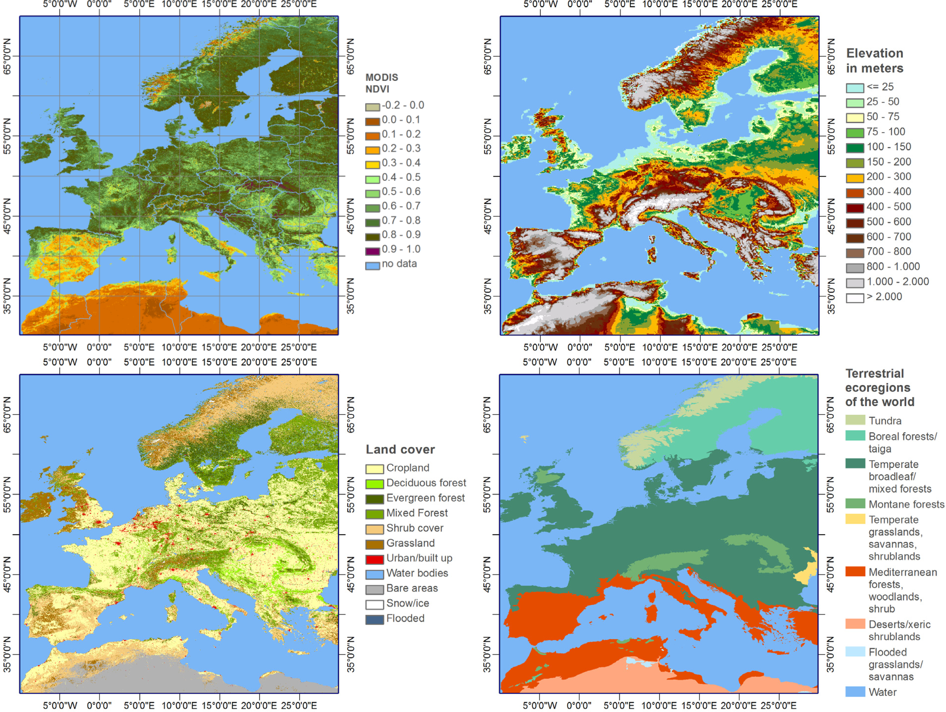
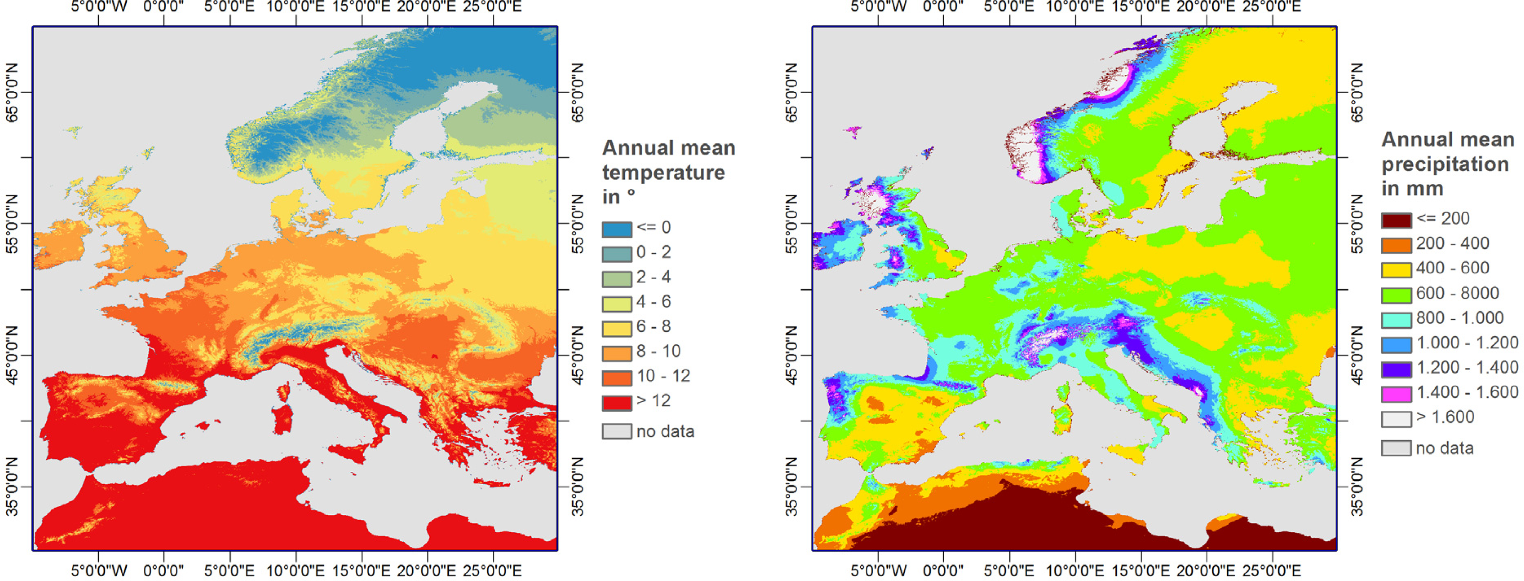
2.1. Study Area
2.2. MODIS Dataset and Temporal Smoothing
2.3. Spatial Degradation of MODIS Data
2.4. GIMMS Dataset
2.5. Temporal Smoothing of GIMMS
2.6. Extraction of Start (SOS) and Maximum of Season (MOS)
- (1)
- Detecting the number of cycles by means of auto-correlation information (e.g., [69]): The number of lags was chosen to be little less than two years. Next the algorithm was searching for maxima and minima on the auto-correlation function (ACF). Two cycles were detected, if a second distinct maximum in the ACF before the end of the year appeared. The maximum was accepted, if the increase before the maximum and decrease after the maximum in the ACF was more than 0.1.
- (2)
- Focus on the first season in case of multiple cycles: If in either of the time series two growing seasons were identified, the algorithm searched for two starts and two maxima each year, while only the first start and maximum was included in the subsequent comparison of the time series.
- (3)
- Defining a temporal search window for each growing season: In a first step the algorithm was searching for the maximum NDVI of each season. The growing season was considered to be centered around the maximum, while the size of the range depends on the number of detected cycles. The start (SOS) will be found between the moment of minimum and the moment of maximum. Even if filtered NDVI curves were used, there might be still several preceding minima. To identify a reasonable and reproducible minimum, the steepest preceding increase was chosen as a criterion. This criterion accounts for the number of increasing time steps and the NDVI difference.
- (4)
3. Results
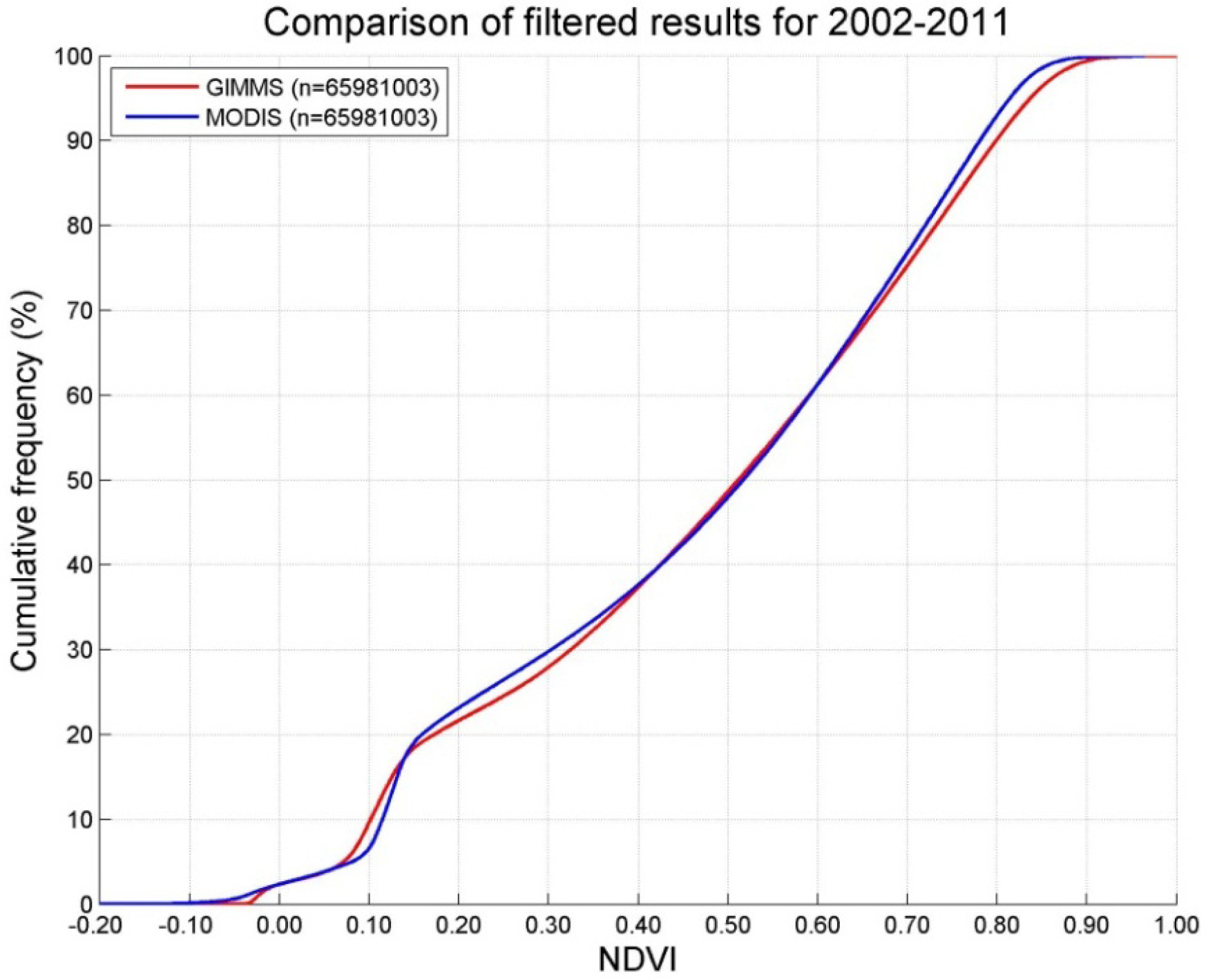
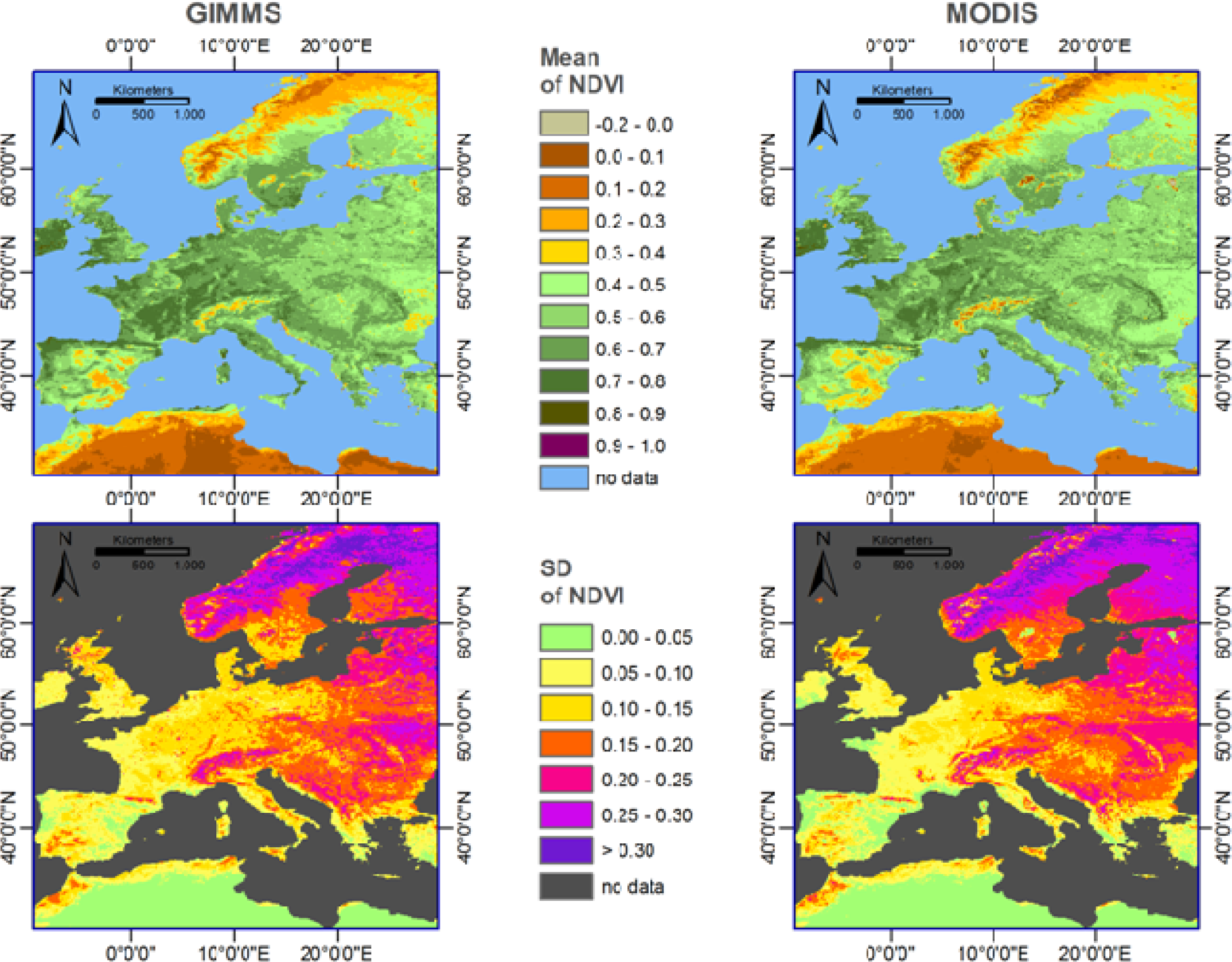
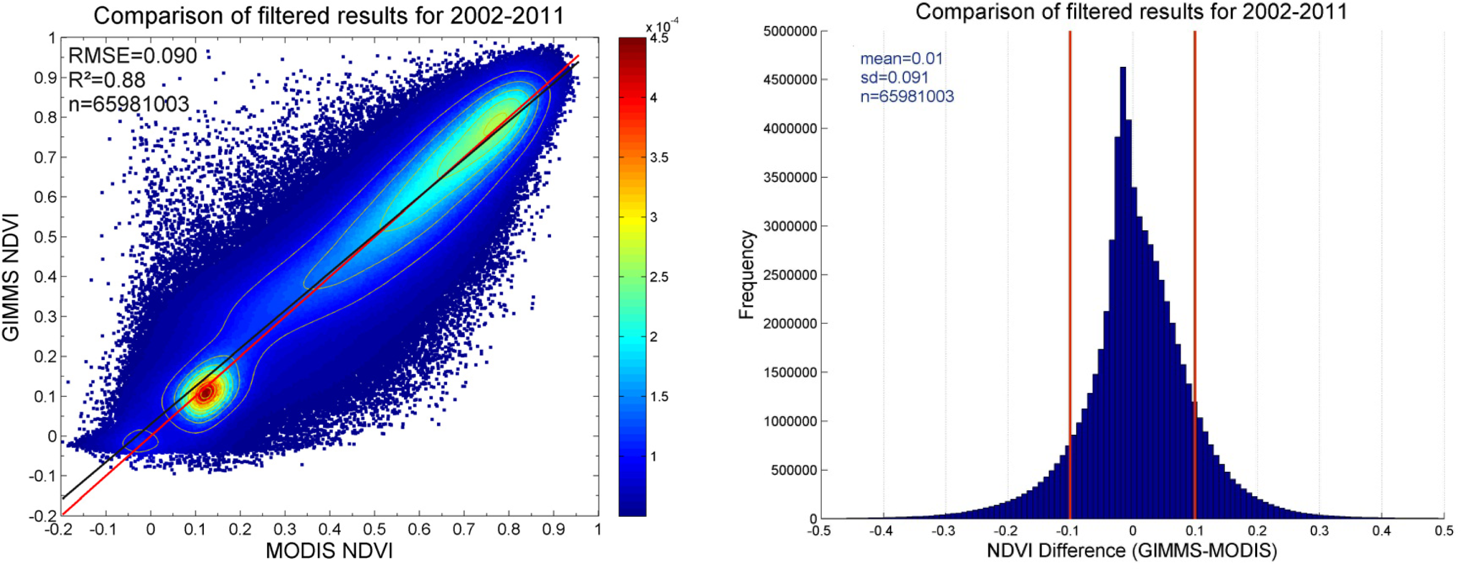
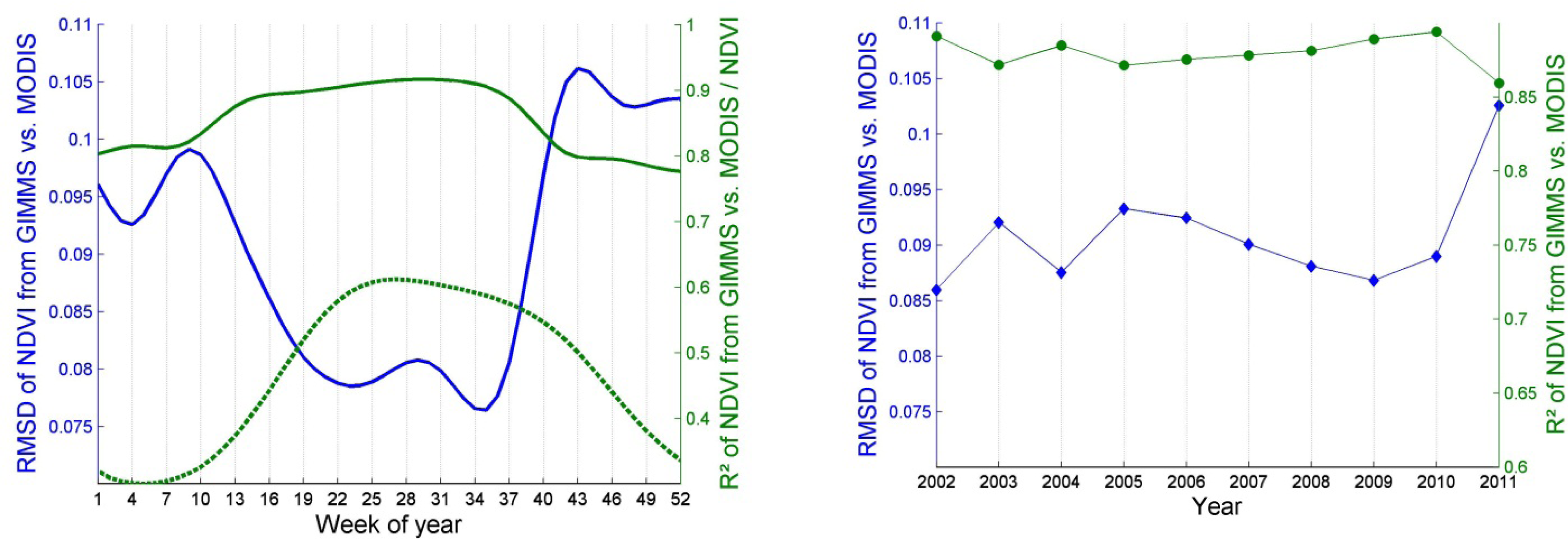
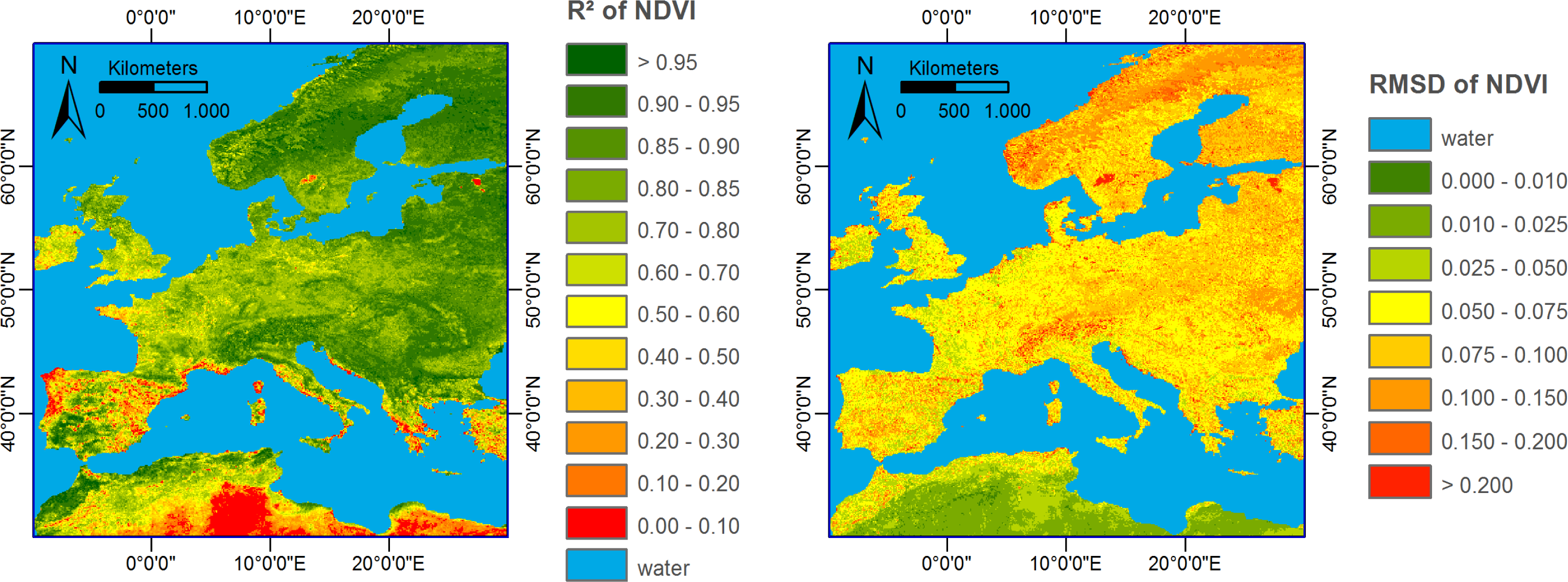
3.1. Data Distribution and Correlation
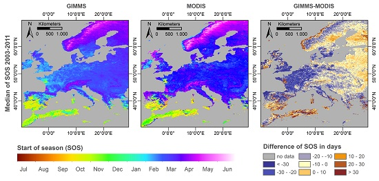
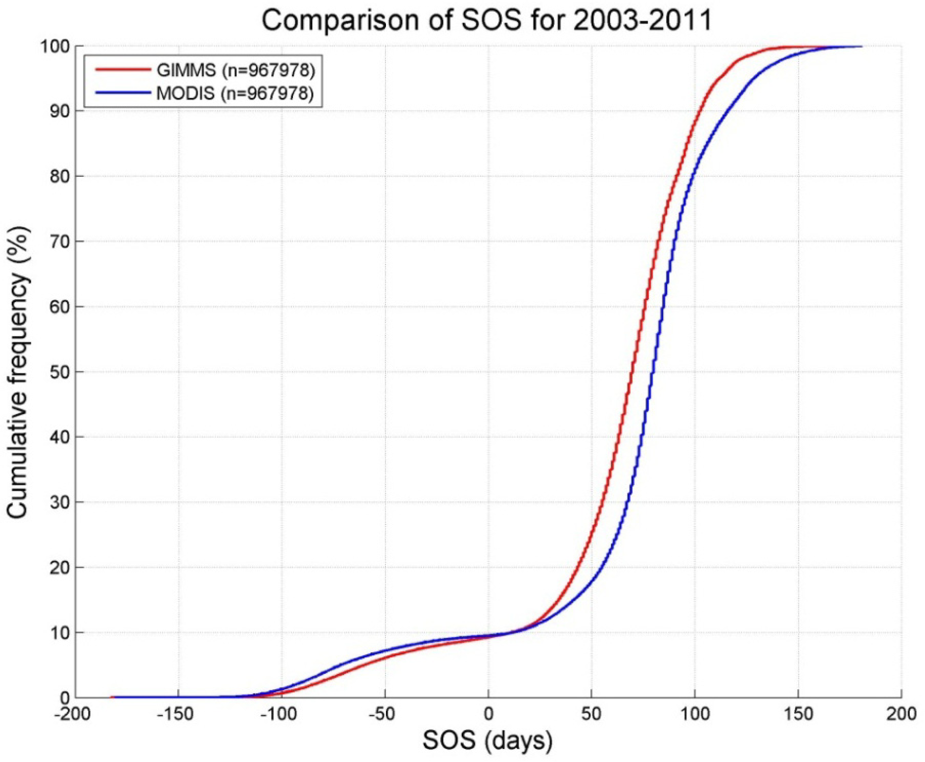
3.2. Phenology: Start of Season (SOS)
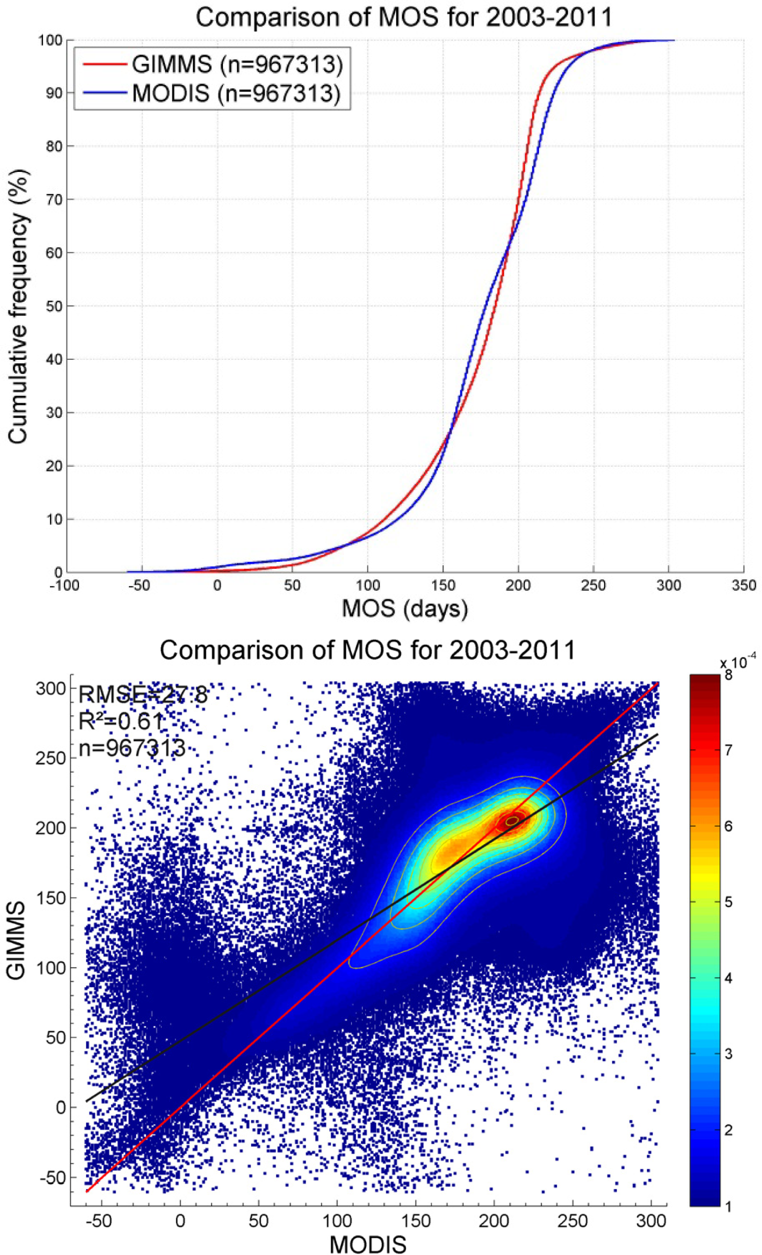
3.3. Phenology: Maximum of Season (MOS)
4. Discussions
5. Conclusions
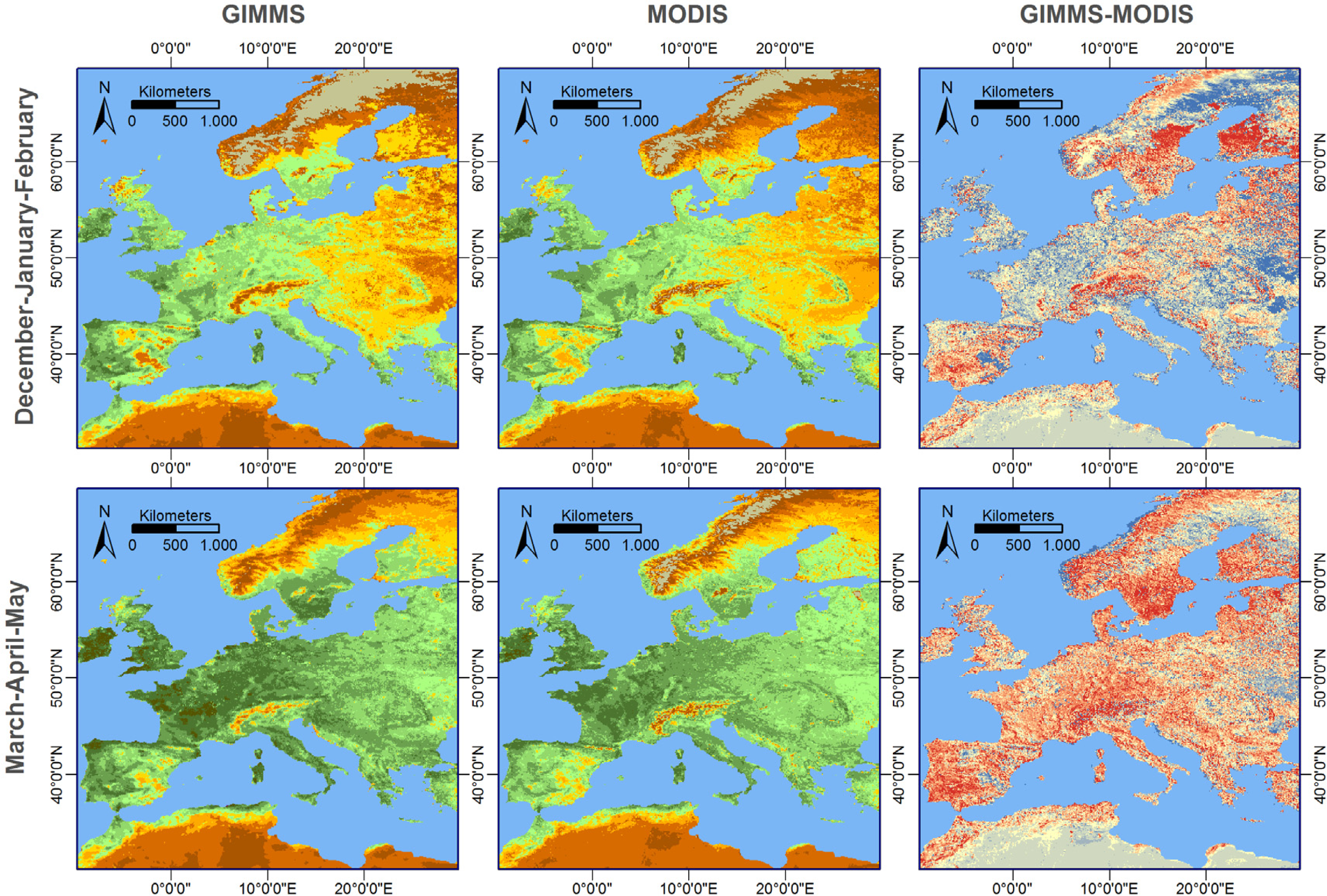
- Overall, the NDVI data sets from GIMMS and MODIS show only a moderately good agreement. Differences in observed vegetation density (NDVI) are largest in winter, followed by autumn. The best agreement is observed during summer. This highlights the need to carefully inter-calibrate the two data sets, giving special attention to autumn and winter. Without such an inter-calibration, the two data sets cannot be analyzed concurrently.
- The maximum of season (MOS) extracted from the two time series shows a good agreement with respect to the observed spatial pattern and its inter-annual variability. However, more research is necessary to explain the observed differences in the timing of vegetation onset (start of season—SOS). GIMMS consistently shows higher vegetation densities during spring. Its temporal NDVI profiles therefore start rising very early in the year and earlier than those of MODIS. This leads to, sometimes, very large differences in the mapped SOS of both data sets. Without removing these differences, the two data sets cannot be combined for phenological studies.
- Regarding the start of season (SOS), differences were observed regarding spatial pattern and inter-annual variation. Only a part of these differences are of systematic nature and could therefore be corrected a posteriori. This again clearly highlights the need of a well-done cross-sensor inter-calibration.
- Future studies should focus on validating phenological indicators. At least for some countries of Europe, long lasting and relative dense phenological networks exist (e.g., Germany and Austria). This permits comparing the remotely sensed indicators against field observations as already shown by e.g., [76–78].
Acknowledgments
Conflicts of Interest
References
- Reed, B.C.; Brown, J.F.; VanderZee, D.; Loveland, T.R.; Merchant, J.W.; Ohlen, D.O. Measuring phenological variability from satellite imagery. J. Veg. Sci 1994, 5, 703–714. [Google Scholar]
- Beck, P.S.A.; Atzberger, C.; Høgda, K.A.; Johansen, B.; Skidmore, A.K. Improved monitoring of vegetation dynamics at very high latitudes: A new method using MODIS NDVI. Remote Sens. Environ 2006, 100, 321–334. [Google Scholar]
- White, M.A.; de Beurs, K.M.; Didan, K.; Inouyes, D.W.; Richardson, A.D.; Jensen, O.P.; O’Keefe, J.; Zhang, G.; Neman, R.R.; van Leeuwen, W.J.D.; et al. Intercomparison, interpretation, and assessment of spring phenology in North America estimated from remote sensing for 1982–2006. Glob. Chang. Biol 2009, 15, 2335–2359. [Google Scholar]
- Tucker, C.J.; Vanpraet, C.; Sharman, M.; van Ittersum, G. Satellite remote sensing of total herbaceous biomass production in the Senegalese Sahel: 1980–1984. Remote Sens. Environ 1985, 17, 233–249. [Google Scholar]
- Atzberger, C. Advances in remote sensing of agriculture: Context description, existing operational monitoring systems and major information needs. Remote Sens 2013, 5, 649–981. [Google Scholar]
- Rembold, F.; Atzberger, C.; Savin, I.; Rojas, O. Using low resolution satellite imagery for yield prediction and yield anomaly detection. Remote Sens 2013, 5, 1704–1733. [Google Scholar]
- Kerr, J.T.; Ostrovsky, M. From space to species: Ecological applications for remote sensing. Trends Ecol. Evol 2003, 18, 299–305. [Google Scholar]
- Anyamba, A.; Eastman, R. Interannual variability of NDVI over Africa and its relation to El Niño/Southern Oscillation. Int. J. Remote Sens 1996, 17, 2533–2548. [Google Scholar]
- Herrmann, S.M.; Anyamba, A. Recent trends in vegetation dynamics in the African Sahel and their relationship to climate. Glob. Environ. Chang 2005, 15, 394–404. [Google Scholar]
- Ji, L.; Peters, A.J. Assessing vegetation response to drought in the northern Great Plains using vegetation and drought indices. Remote Sens. Environ. 2003, 87, 85–98. [Google Scholar]
- Moulin, S.; Kergoat, L.; Viovy, N.; Dedieu, G. Global-scale assessment of vegetation phenology using NOAA/AVHRR satellite measurements. J. Clim 1997, 10, 1154–1170. [Google Scholar]
- Jönsson, P.K.; Eklundh, L. Seasonality extraction by function fitting to time series of satellite sensor data. IEEE Trans. Geosci. Remote Sens 2002, 40, 1824–1832. [Google Scholar]
- Stöckli, R.; Vidale, P. European plant phenology and climate as seen in a 20-year AVHRR land-surface parameter dataset. Int. J. Remote Sens 2004, 25, 3303–3330. [Google Scholar]
- Li, Z.; Kafatos, M. Interannual variability of vegetation in the United States and its relation to El Niño/Southern Oscillation. Remote Sens. Environ 2000, 41, 239–247. [Google Scholar]
- Tucker, C.J.; Slayback, D.A.; Pinson, J.E.; Los, S.O.; Myneni, R.B.; Taylor, M.G. Higher northern latitude normalized difference vegetation index and growing season trends from 1982 to 1999. Int. J. Biometeorol 2001, 45, 184–190. [Google Scholar]
- Shabanov, N.V.; Zhou, L.; Knyazikhin, Y.; Myneni, R.B.; Tucker, C.J. Analysis of interannual changes in northern vegetation activity observed in AVHRR data from 1981 to 1994. IEEE Trans. Geosci. Remote Sens 2002, 40, 115–130. [Google Scholar]
- Piao, S.; Fang, J.; Zhou, L.; Ciais, P.; Zhu, B. Variations in satellite-derived phenology of China’s temperate vegetation. Glob. Chang. Biol 2006, 12, 672–685. [Google Scholar]
- Friedl, M.A.; Brodley, C.E.; Strahler, A.H.; R, I.N. Maximizing land cover classification accuracies produced by decision trees at continental to global scales. IEEE Trans. Geosci. Remote Sens 1999, 3, 969–977. [Google Scholar]
- Hansen, M.C.; Defries, R.S.; Townshend, J.R.G.; Sohlberg, R. Global land cover classification at 1 km spatial resolution using a classification tree approach. Int. J. Remote Sens 2000, 21, 1331–1364. [Google Scholar]
- Xiao, X.; Bolesa, S.; Liub, J.; Zhuangb, D.; Frolkinga, S.; Lia, C.; Salasc, W.; Moore, B. Mapping paddy rice agriculture in southern China using multi-temporal MODIS images. Remote Sens. Environ 2005, 95, 480–492. [Google Scholar]
- Xavier, A.C.; Rudorff, B.F.T.; Shimabukuro, Y.E.; Berka, L.M.S.; Moreira, M.A. Multi-temporal analysis of MODIS data to classify sugarcane crop. Int. J. Remote Sens 2006, 27, 755–768. [Google Scholar]
- Wardlow, B.; Egbert, S.; Kastens, J. Analysis of time-series MODIS 250 m vegetation index data for crop classification in the U.S. Central Great Plains. Remote Sens. Environ 2007, 108, 290–310. [Google Scholar]
- Vuolo, F.; Atzberger, C. Exploiting the classification performance of support vector machines with multi-temporal Moderate-Resolution Imaging Spectroradiometer (MODIS) data in areas of agreement and disagreement of existing land cover products. Remote Sens 2012, 4, 3143–3167. [Google Scholar]
- Eastman, R.J.; Fulk, M. Long sequence time series evaluation using standardized principal components. Photogramm. Eng. Remote Sens 1993, 59, 991–996. [Google Scholar]
- Azzali, S.; Menenti, M. Mapping vegetation-soil-climate complexes in southern Africa using temporal Fourier analysis of NOAA-AVHRR NDVI data. Int. J. Remote Sens 2000, 21, 973–996. [Google Scholar]
- Paruelo, J.M.; Burke, I.C.; Lauenroth, W.K. Land-use impact on ecosystem functioning in eastern Colorado, USA. Glob. Chang. Biol 2001, 7, 631–639. [Google Scholar]
- Martínez, B.; Gilabert, M.A. Vegetation dynamics from NDVI time series analysis using the wavelet transform. Remote Sens. Environ 2009, 113, 1823–1842. [Google Scholar]
- Atzberger, C.; Eilers, P.H.C. A time series for monitoring vegetation activity and phenology at 10-daily time steps covering large parts of South America. Int. J. Digit. Earth 2011, 4, 365–386. [Google Scholar]
- Geerken, R.A. An algorithm to classify and monitor seasonal variations in vegetation phenologies and their inter-annual change. ISPRS J. Photogramm. Remote Sens 2009, 64, 422–431. [Google Scholar]
- Hurlbert, A.H.; Haskell, J.P. The effect of energy and seasonality on avian species richness and community composition. Am. Nat 2003, 161, 83–97. [Google Scholar]
- Pettorelli, N.; F. Pelletier, A.; von Hardenberg, M.F.B.; CôTé, S.D. Early onset of vegetation growth vs. rapid green-up: Impacts on juvenile mountain ungulates. Ecology 2007, 88, 381–390. [Google Scholar]
- Scharlemann, J.P.W.; Benz, D.; Hay, S.I.; Purse, B.V.; Tatem, A.J.; Wint, G.R.W.; Rogers, D.J. Global data for ecology and epidemiology: A novel algorithm for temporal Fourier processing MODIS data. PLoS ONE 2008, 3, e1408. [Google Scholar]
- Coops, N.; Wulder, M.; Iwanicka, D. An environmental domain classification of Canada using earth observation data for biodiversity assessment. Ecol. Inform 2009, 4, 8–22. [Google Scholar]
- Fuller, D. Trends in NDVI time series and their relation to rangeland and crop production in Senegal, 1987–1993. Int. J. Remote Sens 1998, 19, 2013–2018. [Google Scholar]
- Zhang, P.; Anderson, B.; Tan, B.; Huang, D.; Myneni, R. Potential monitoring of crop production using a satellite-based Climate-Variability Impact Index. Agric. For. Meteorol 2005, 132, 344–358. [Google Scholar]
- McVicar, T.R.; Jupp, D.L. The current and potential operational uses of remote sensing to aid decisions on drought exceptional circumstances in Australia: A review. Agric. Syst 1998, 57, 399–468. [Google Scholar]
- Barbosa, P.; Stroppiana, D.; Pereira, J. An algorithm for extracting burned areas from time series of AVHRR GAC data applied at a continental scale. Remote Sens. Environ 1999, 69, 38–49. [Google Scholar]
- Fraser, R.H.; Li, Z.; Cihlar, J. Hotspot and NDVI Differencing Synergy (HANDS): A new technique for burned area mapping over boreal forest. Remote Sens. Environ 2000, 74, 362–376. [Google Scholar]
- Coops, N.C.; Wulder, M.A.; Iwanicka, D. Large area monitoring with a MODIS-based Disturbance Index (DI) sensitive to annual and seasonal variations. Remote Sens. Environ 2009, 113, 1250–1261. [Google Scholar]
- Spanner, M.; Pierce, L.; Running, S.; D.L., P. The seasonality of AVHRR data of temperate coniferous forests: Relationship with leaf area index. Remote Sens. Environ 1990, 33, 97–112. [Google Scholar]
- Sellers, P.J.; Tucker, C.J.; Collatz, G.J.; Los, S.O.; Justice, C.O.; Dazlich, D.A.; Randall, D.A. A global 1° by 1° NDVI data set for climate studies. Part 2: The generation of global fields of terrestrial biophysical parameters from the NDVI. Int. J. Remote Sens 1994, 15, 3519–3545. [Google Scholar]
- Huete, A.; Didan, K.; Miura, T.; Rodriguez, E.P.; Gao, X.; Ferreira, L.G. Overview of the radiometric and biophysical performance of the MODIS vegetation indices. Remote Sens. Environ 2002, 83, 195–213. [Google Scholar]
- Wang, Q.; Adiku, S.; Tenhunen, J.; Granier, A. On the relationship of NDVI with leaf area index in a deciduous forest site. Remote Sens. Environ 2005, 94, 244–255. [Google Scholar]
- Pinzón, J. Revisiting error, precision and uncertainty in NDVI AVHRR data: Development of a consistent NDVI3g time series. Remote Sens 2013. under review.. [Google Scholar]
- Van Leeuwen, W.J.D.; Orr, B.J.; Marsh, S.E.; Herrmann, S.M. Multi-sensor NDVI data continuity: Uncertainties and implications for vegetation monitoring applications. Remote Sens. Environ 2006, 100, 67–81. [Google Scholar]
- Meroni, M.; Atzberger, C.; Vancutsem, C.; Gobron, N.; Baret, F.; Lacaze, R.; Eerens, H.; Leo, O. Evaluation of agreement between space remote sensing SPOT-VEGETATION fAPAR time series. IEEE Trans. Geosci. Remote Sens 2013, 51, 1951–1962. [Google Scholar]
- Mao, J.; Shi, X.; Thornton, P.E.; Hoffman, F.M.; Zhu, Z.; Myneni, R.B. Global latitudinal-asymmetric vegetation growth trends and their driving mechanisms: 1982–2009. Remote Sens 2013, 5, 1484–1497. [Google Scholar]
- De Jong, R.; Verbesselt, J.; Zeileis, A.; Schaepman, M.E. Shifts in global vegetation activity trends. Remote Sens 2013, 5, 1117–1133. [Google Scholar]
- Vrieling, A.; de Leeuw, J.; Said, M.Y. Length of growing period over Africa: Variability and trends from 30 Years of NDVI time series. Remote Sens 2013, 5, 982–1000. [Google Scholar]
- Brown, M.E.; Pinzon, J.E.; Didan, K.; Morisette, J.T.; Tucker, C.J. Evaluation of the consistency of long-term NDVI time series derived from AVHRR, SPOT-Vegetation, Sea WiFS, MODIS, and LandSAT ETM+ sensors. IEEE Trans. Geosci. Remote Sens 2006, 44, 1787–1793. [Google Scholar]
- Justice, C.; Belward, A.; Morisette, J.; Lewis, P.; Privette, J.; Baret, F. Developments in the ‘validation’ of satellite sensor products for the study of the land surface. Int. J. Remote Sens 2000, 51, 3383–3390. [Google Scholar]
- Garrigues, S.; Lacaze, R.; Baret, F.; Morisette, J.T.; Weiss, M.; Nickeson, J.E.; Fernandes, R.; Plummer, S.; Shabanov, N.V.; Myneni, R.B.; et al. Validation and intercomparison of global Leaf Area Index products derived from remote sensing data. J. Geophys. Res 2008, 113, G02028. [Google Scholar]
- Baret, F.; Morissette, J.; Fernandes, R.; Champeaux, J.; Myneni, R.; Chen, J.; Plummer, S.; Weiss, M.; Bacour, C.; Garrigues, S.; et al. Evaluation of the representativeness of networks of sites for the global validation and intercomparison of land biophysical products: proposition of the CEOS-BELMANIP. IEEE Trans. Geosci. Remote Sens 2006, 44, 1794–1803. [Google Scholar]
- Morisette, J.T.; Baret, F.; Privette, J.L.; Myneni, R.B.; Nickeson, J.E.; Garrigues, S.; Shabanov, N.V.; Weiss, M.; Fernandes, R.; Leblanc, S.G.; et al. Validation of global moderate-resolution LAI products: A framework proposed within the CEOS land product validation subgroup. IEEE Trans. Geosci. Remote Sens 2006, 44, 1804–1818. [Google Scholar]
- Weiss, M.; Baret, F.; Garrigues, S.; Lacaze, R. LAI and fAPAR CYCLOPES global products derived from VEGETATION. Part 2: Validation and comparison with MODIS collection 4 products. Remote Sens. Environ 2007, 110, 317–331. [Google Scholar]
- NOAA. Data Announcement 88-MGG-02, Digital Relief of the Surface of the Earth; National Geophysical Data Center, NOAA: Boulder, CO, USA, 1988. [Google Scholar]
- Olson, D.; Dinerstein, E.; Wikramanayake, E.; Burgess, N.; Powell, G.; Underwood, E.; D’Amico, J.; Itoua, I.; Strand, H.; Morrison, J.; et al. Terrestrial Ecoregions of the World: A New Map of Life on Earth. BioScience 2001, 51, 933–938. [Google Scholar]
- Hijmans, R.; Cameron, S.; Parra, J.; Jones, P.; Jarvis, A. Very high resolution interpolated climate surfaces for global land areas. Int. J. Clim 2005, 25, 1965–1978. [Google Scholar]
- Kottek, M.; Grieser, J.; Beck, C.; Rudolf, B.; Rubel, F. World map of Köppen-Geiger climate classification updated. Meteorol. Z 2006, 15, 259–263. [Google Scholar]
- Friedl, M.A.; Sulla-Menashe, D.; Tan, B.; Schneider, A.; Ramankutty, N.; Sibley, A.; Huang, X. MODIS Collection 5 global land cover: Algorithm refinements and characterization of new datasets. Remote Sens. Environ 2010, 114, 168–182. [Google Scholar]
- Solano, R.; Didan, K.; Jacobson, A.; Huete, A. MODIS Vegetation Index User’s Guide (MOD13 Series); Version 2.00, May 2010 (Collection 5); The University of Arizona: Tucson, AZ, USA, 2010. [Google Scholar]
- Mattiuzzi, M.; Verbesselt, J.; Hengl, T.; Klisch, A.; Evans, B.; Lobo, A. MODIS Multi-Temporal Data Retrieval and Processing Toolbox. Processing of First International Workshop on “Temporal Analysis of Satellite Images”, Mykonos Island, Greece, 23–25 May 2012.
- Vuolo, F.; Mattiuzzi, M.; Klisch, A.; Atzberger, C. Data service platform for MODIS vegetation indices time series processing at BOKU Vienna: Current status and future perspectives. Proc. SPIE 2012, 8538. [Google Scholar] [CrossRef]
- Atzberger, C.; Eilers, P.H.C. Evaluating the effectiveness of smoothing algorithms in the absence of ground reference measurements. Int. J. Remote Sens 2011, 32, 3689–3709. [Google Scholar]
- Eilers, P.H.C. A perfect smoother. Anal. Chem 2003, 75, 3631–3636. [Google Scholar]
- Atkinson, P.M.; Jeganathan, C.; Dash, J.; Atzberger, C. Intercomparison of four models for smoothing satellite sensor time-series data to estimate vegetation phenology. Remote Sens. Environ 2012, 123, 400–417. [Google Scholar]
- Fensholt, R.; Proud, S.R. Evaluation of Earth Observation based global long term vegetation trends—Comparing GIMMS and MODIS global NDVI time series. Remote Sens. Environ 2012, 119, 131–147. [Google Scholar]
- Tucker, C.; Pinzon, J.; Brown, M.; Slayback, D.; Pak, E.; Mahoney, R.; Vermote, E.; Saleous, E. An extended AVHRR 8-km NDVI dataset compatible with MODIS and SPOT vegetation NDVI data. Int. J. Remote Sens 2005, 26, 4485–4498. [Google Scholar]
- Verstraete, M.M.; Gobron, N.; Aussedat, O.; Robustelli, M.; Pinty, B.; Widlowski, J.L.; Taberner, M. An automatic procedure to identify key vegetation phenology events using the JRC-FAPAR products. Adv. Space Res 2008, 41, 1773–1783. [Google Scholar]
- Delbart, N.; Le Toan, L.; Kergoat, L.; Fedotova, V. Remote sensing of spring phenology in boreal regions: A free of snow-effect method using NOAA-AVHRR and SPOT-VGT data (1982–2004). Remote Sens. Environ 2006, 101, 52–62. [Google Scholar]
- Van Leeuwen, W.J.D. Monitoring the effects of forest restoration treatments on post-fire vegetation recovery with MODIS multitemporal data. Sensors 2008, 8, 2017–2042. [Google Scholar]
- De Beurs, K.; Henebry, G. Spatio-Temporal Statistical Methods for Modeling Land Surface Phenology. In Phenological Research: Methods for Environmental and Climate Change Analysis; Hudson, I.L., Keatley, M.R., Eds.; Springer: Berlin, Germany, 2010; pp. 177–208. [Google Scholar]
- Karlsen, S.R.; Høgda, K.; Johansen, B.; Elvebakk, A.; Tømmervik, H. Use of AVHRR NDVI Data to Map Vegetation Zones in North-Western Europe. Proceedings of the 29th International Symposium on Remote Sensing Environment (ISRSE), Buenos Aires, Argentina, 8–12 April 2002.
- Karlsen, S.R.; Ramfjord, H.; Høgda, K.A.; Johansen, B.; Danks, F.S.; Brobakk, T.E. A satellite-based map of onset of birch (Betula) flowering in Norway. Aerobiologica 2009, 25, 15–25. [Google Scholar]
- Beck, P.S.A.; Jönsson, P.; Høgda, K.A.; Karlsen, S.R.; Eklundh, L.; Skidmore, A.K. A ground-validated NDVI dataset for monitoring vegetation dynamics and mapping phenology in Fennoscandia and the Kola Peninsula. Int. J. Remote Sens 2007, 28, 4311–4330. [Google Scholar]
- Soudani, K.; le Maire, G.; Dufrêne, E.; Francois, C.; Delpierre, N.; Ulrich, E.; Cecchini, S. Evaluation of the onset of green-up in temperate deciduous broadleaf forests derived from Moderate Resolution Imaging Spectroradiometer (MODIS) data. Remote Sens. Environ 2008, 112, 2643–2655. [Google Scholar]
- Bradley, C.; Schwartz, M.; Xiao, X. Remote Sensing Phenology: Status and Way forward. In Phenology of Ecosystem Processes—Applications in Global Change Research; Springer: Berlin, Germany, 2009; pp. 231–246. [Google Scholar]
- Liang, L.; Schwartz, M.D.; Fei, S. Validating satellite phenology through intensive ground observation and landscape scaling in a mixed seasonal forest. Remote Sens. Environ 2011, 115, 143–157. [Google Scholar]


| Type of Application | Reference |
|---|---|
| Seasonality extraction and vegetation dynamics | [1–3,11–13] |
| Environmental monitoring and climate change | [8,9,14–17] |
| Land use and land cover mapping | [18–23] |
| Vegetation and landscape characterization | [24–29] |
| Biodiversity and wildlife distribution | [4,7,30–33] |
| Primary production and yield/production estimates | [4,6,34,35] |
| Drought monitoring and food security | [10,36] |
| Change detection (incl. natural disasters, forest fires) | [37–39] |
| Characterizing vegetation’s biophysical variables | [40–43] |
| Parameterization of the Whittaker Smoother for Providing Smoothed Weekly Data | Spatial Resampling | Land/Water Masking | |||||
|---|---|---|---|---|---|---|---|
| λ ×103 | Degree | n° of Iterations | Compositing Day | Quality Flags | |||
| GIMMS | 30 | 2nd | 1 | Not available | Not considered | Original sampling at 1/12 degrees is kept | Common masks applied to both data sets |
| MODIS | 30 | 2nd | 3 | True DOY considered | Considered | Average resampling to 1/12 degrees | |
© 2014 by the authors; licensee MDPI, Basel, Switzerland This article is an open access article distributed under the terms and conditions of the Creative Commons Attribution license ( http://creativecommons.org/licenses/by/3.0/).
Share and Cite
Atzberger, C.; Klisch, A.; Mattiuzzi, M.; Vuolo, F. Phenological Metrics Derived over the European Continent from NDVI3g Data and MODIS Time Series. Remote Sens. 2014, 6, 257-284. https://doi.org/10.3390/rs6010257
Atzberger C, Klisch A, Mattiuzzi M, Vuolo F. Phenological Metrics Derived over the European Continent from NDVI3g Data and MODIS Time Series. Remote Sensing. 2014; 6(1):257-284. https://doi.org/10.3390/rs6010257
Chicago/Turabian StyleAtzberger, Clement, Anja Klisch, Matteo Mattiuzzi, and Francesco Vuolo. 2014. "Phenological Metrics Derived over the European Continent from NDVI3g Data and MODIS Time Series" Remote Sensing 6, no. 1: 257-284. https://doi.org/10.3390/rs6010257