Training Area Concept in a Two-Phase Biomass Inventory Using Airborne Laser Scanning and RapidEye Satellite Data

Abstract

This study evaluated the accuracy of boreal forest above-ground biomass (AGB) and volume estimates obtained using airborne laser scanning (ALS) and RapidEye data in a two-phase sampling method. Linear regression-based estimation was employed using an independent validation dataset and the performance was evaluated by assessing the bias and the root mean square error (RMSE). In the phase I, ALS data from 50 field plots were used to predict AGB and volume for the 200 surrogate plots. In the phase II, the ALS-simulated surrogate plots were used as a ground-truth to estimate AGB and volume from the RapidEye data for the study area. The resulting RapidEye models were validated against a separate set of 28 plots. The RapidEye models showed a promising accuracy with a relative RMSE of 19%–20% for both volume and AGB. The evaluated concept of biomass inventory would be useful to support future forest monitoring and decision making for sustainable use of forest resources.

1. Introduction

Forests play an important role in global carbon cycling, since the world’s forests sequestrate and conserve more carbon than all other terrestrial ecosystems, and account for 90% of the annual carbon flux between the atmosphere and the Earth’s land surface [1]. Accurate estimation of forest biomass is required for countries ratifying the Kyoto Protocol to the United Nations Framework Convention on Climate change [2]. Assessment of biomass within all compartments of forest ecosystems can be achieved by choosing the appropriate scientific techniques. The combination of remote sensing with ground surveys potentially offers way to guarantee accurate monitoring, reporting and verification of terrestrial forest biomass [3–5]. Southworth and Gibbes [6] reviewed the past, present and future directions of remote sensing applications in the forestry sector. They concluded that the fusion of different remote sensing techniques is promising for the monitoring and assessing of forest ecosystems.

The estimation of forest carbon is still relatively uncertain considering the errors in regional carbon stock estimates. Houghton [7] mentioned that 89% of the carbon losses are due to the loss of living biomass; therefore, attempts have been centered on estimating the above-ground biomass (AGB) of vegetation [8]. Accurate large-scale estimation of AGB using active or passive remote sensing has been a significant challenge to forest scientists; however, it is crucial for future implementation of carbon credit verification in the Land-Use Change and Forestry (LUCF) sector [9]. The purpose of verifying forest biomass inventory is to establish their reliability and to monitor the accuracy of the numbers reported by independent means.

Finland, the northernmost European country, has 73% of its land area forested [10]. In Finnish boreal forests, coniferous trees represent over 80% of the growing stock. Globally, boreal forests are of particular interest because among all the biomes, they may undergo the greatest climatically induced changes during the 21st century [11]. Boreal coniferous forests are the largest terrestrial biome on Earth and store 31 × 10¹² kg of carbon in the trees alone [12]. Research indicates that the boreal forests are more significant as carbon sinks than has been thought previously [12,13].

A wide range of approaches have been proposed for quantifying forest biomass using active and passive remote sensing systems. Although many alternative remote sensing techniques have been suggested for the estimation of forest attributes such as AGB, the most promising one seems to be the airborne laser scanning (ALS) [14]. ALS sensors provide accurate information on the 3D structure of the vegetation, as they directly measure distances to the targets below. ALS has potential to increase accuracy and reduce costs in large-scale forest inventories [13–17]. The two established approaches for predicting forest biomass using ALS are the area-based method (ABM) and the individual tree delineation (ITD). Both approaches have been proven to provide competent results, but large-scale applications are usually conducted using the ABM [18]. In this approach, field-measured data and ALS metrics are used to make statistical models that describe the relationship between ALS metrics (used as predictors) and field-measured forest properties (e.g., AGB).

The RapidEye is a multispectral satellite sensor launched on 2008 with an ability to acquire images with high spatial resolution (5 m) on five spectral bands. The RapidEye images have been used in several forestry operations, including cost-effective monitoring, harvesting and mapping [19,20]. The RapidEye data might be easier to obtain in many countries than other remotely sensed data, such as ALS data. The drawback of all optical satellite images in the estimation of biomass is the saturation of predicted values at dense leaf canopies, which restricts the estimates to low biomass levels [21,22].

The most commonly used features derived from the optical data to predict forest attributes are the spectral and textural features. Spectral features describe the tonal variation in portions of the electromagnetic spectrum. Textural features contain information about the spatial distribution of tonal variations within an image. Texture has qualities such as periodicity and scale; it can therefore describe, for example, the direction, coarseness, and contrast of image components [23]. The combination of spectral and textural features has provided better accuracy in the estimation of forest attributes than the use of any feature alone. Haralick et al. [24] presented the use of grey-level co-occurrence matrices in quantifying the texture. Their method has been widely used in remote sensing-based forestry applications [25,26].

Albeit the costs of ALS data have decreased considerably, it has relatively high cost compared to the optical sensors. Decreasing the number of field reference plots to minimize the costs of data collection is desirable, as the cost of field measurements was estimated to be around 100 € per sample plots (9 m radius) in Finland [27]. Tegel [28] mentioned that if the number of field reference plots is not sufficient, the accuracy of large-sale inventory results can be improved by combining satellite imagery with ALS data and field measurements, instead of using just the field plots.

The objective of this study was to assess the AGB and volume using ALS data and RapidEye satellite data in a two-phase sampling procedure. ALS-estimated sample plots (called surrogate plots) were used as a simulated ground-truth instead of more expensive field sample plots. A small number of field sample plots were collected to create ALS-based models, which were applied to predict the AGB and volume for the surrogate plots. Finally, RapidEye image and the surrogate plots were used to generalize the predictions for the study area.

The accuracy of the predictions was evaluated by means of root mean square error (RMSE) and bias. To our knowledge, there are few studies focused on using ALS data as a simulated ground-truth for the satellite-based forest inventory (e.g., [22]). This study is aimed at obtaining an overall view on the accuracy of two-phase biomass inventory using ALS and RapidEye satellite data.

2. Materials

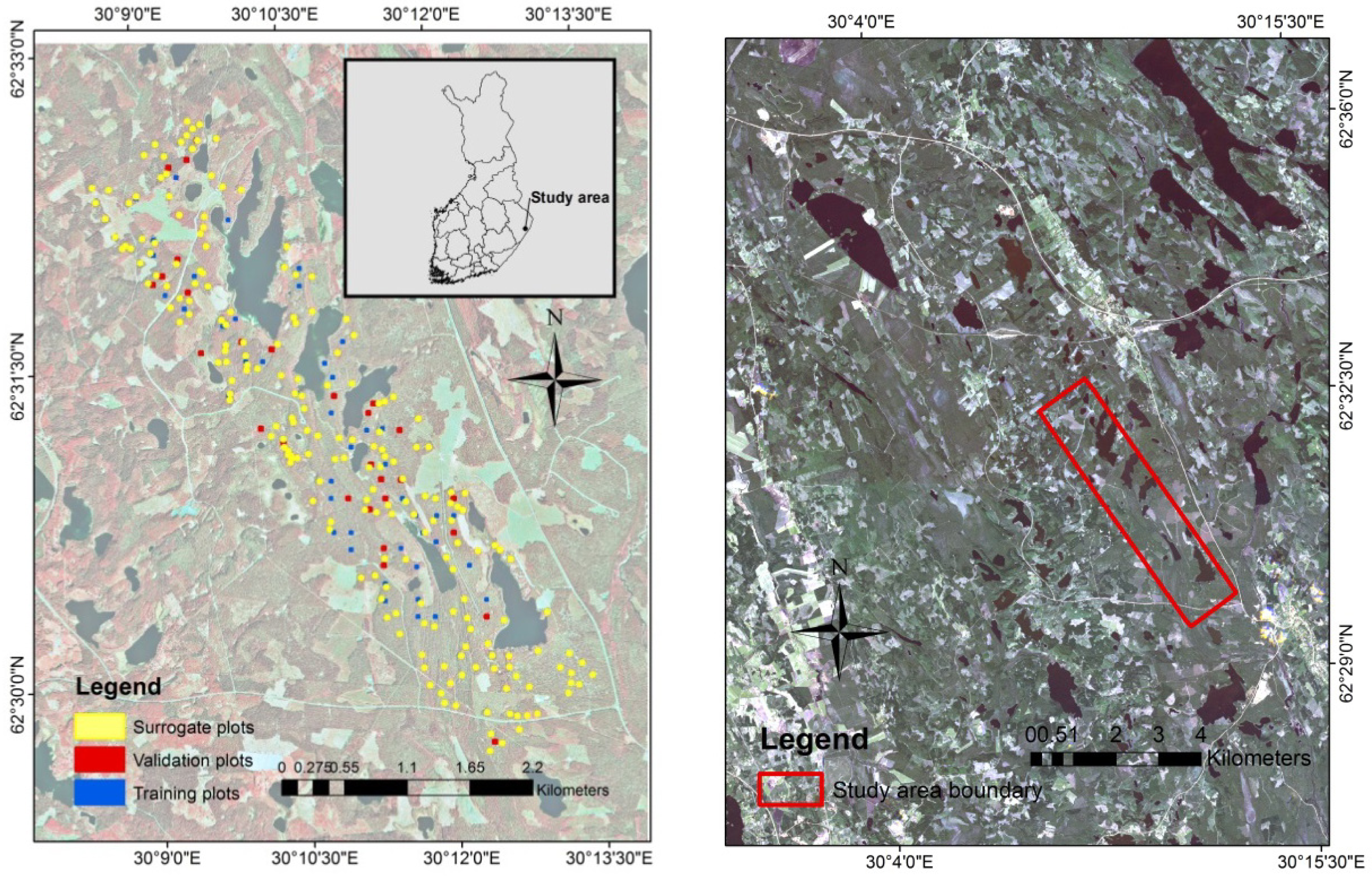
2.1. Study Area and Field Data

The study area is located in eastern Finland (62°31′N, 30°10′E) (Figure 1). The boreal forests of the area are managed for timber production and ecological sustainability. Scots pine (Pinus sylvestris L.) is the dominant tree species, representing 73% of the volume. Norway spruce (Picea abies L.) represents 16% of the volume, and rest come from deciduous trees such as downy birch (Betula pubescens Ehrh.) and silver birch (Betula pendula Roth.), which usually occur as minor species.

The field measurements were carried out in May to June 2010. Altogether, 78 field plots were placed subjectively into different stands in an attempt to record the species and size variation over the area. The field plots were placed into the area subjectively based on the development class and dominant tree species. The sizes of the field plots ranged from 20 × 20 to 30 × 30 m. Field sample plots were divided into training (n = 50) (phase I) and validation (n = 28) data sets; the training set comprised the plots whose size was 25 × 25 m (0.065 ha). The other plots with varying sizes were used for validation. It is worth noting that the larger sample plots maintain a greater amount of spatial overlap, minimize the edge effects, and increase the sample variances [29].

A total of 200 surrogate plots (35 × 35 m) were placed to cover the study area using an ortho-rectified aerial photograph with the green, red and near-infrared portions of the spectrum. These plots were used as a simulated ground-truth and while training the RapidEye models in the phase II (described in Section 3.4). We used visual interpretation of aerial photographs in the placement of the surrogate plots. The idea was that the surrogate plots should cover all the variation (i.e., vegetation type, geographic location, species composition) in the study area.

All trees with either diameter at breast height (DHB) ≥ 4 cm or height ≥ 4 m were measured in the field. The volumes of the individual trees were calculated as a function of diameter at breast height (DBH) and tree height using species-specific models [30]. The AGB of individuals trees was calculated by using the biomass Equations (1–3) developed by Repola [31,32], respectively, for Scots pine, Norway spruce and deciduous. Repola [31,32] applied a multivariate mixed linear model in biomass predictions and the equations are as follows:

$$\text{ln}(y_{\mathit{ki}})=b_0+b_1\frac{d_{\mathit{ski}}}{(d_{\mathit{ski}}+12)}+b_2\frac{h_{\mathit{ki}}}{(h_{\mathit{ki}}+20)}+u_k+e_{\mathit{ki}}$$

(1)

$$\text{ln}(y_{\mathit{ki}})=b_0+b_1\frac{d_{\mathit{ski}}}{(d_{\mathit{ski}}+20)}+b_2\text{ln}(h_{\mathit{ki}})+u_k+e_{\mathit{ki}}$$

(2)

$$\text{ln}(y_{\mathit{ki}})=b_0+b_1\frac{d_{\mathit{ski}}}{(d_{\mathit{ski}}+12)}+b_2\frac{h_{\mathit{ki}}}{(h_{\mathit{ki}}+22)}+u_k+e_{\mathit{ki}}$$

(3)

where y_ki is the total AGB (kg) of tree i in stand k, b₀, b₁ and b₂ are the vectors of fixed effects parameters, d_ski is (2 + 1.25 × DBH), h_ki is the height (m) of tree, u_k is the variance of random parameters, and e_ki is the residual error.

Table 1. Estimates of multivariate model fixed parameters, and variances of random stand parameters (u_k) and residual errors (e_ki) [31,32].

Parameters	Scots Pine	Norway Spruce	Deciduous
Fixed effects
b0	−3.1	−1.8	−3.6
b1	9.5	9.4	10.5
b2	3.2	0.4	3.0
Random effects
uk	0.009	0.006	0.00068
eki	0.010	0.013	0.000727

shows the multivariate model fixed parameters and residual errors values. Finally, total volume and AGB were calculated for each plot and stands per hectare. The characteristics of the training plots and validation stands are presented in

Table 2. The mean characteristics of the training plots and validation plots.

	Minimum	Maximum	Mean	SD
Training plots, n = 50
Total volume (m3/ha)	96.1	433.8	209.3	74.9
AGB (ton/ha)	51.5	226.6	113.0	39.7
Validation plots, n = 28
Total volume (m3/ha)	103.6	382.5	219.1	69.0
AGB (ton/ha)	55.9	182.2	115.7	31.5

.

2.2. Remote Sensing Data

The ALS data was collected on 18 July 2009 using an Optech ALTM Gemini laser scanning system. The nominal pulse density was about 0.65 per square meter. The test site was scanned from an altitude that is approximately 2000 m above ground level with a field view of 30 degrees and side overlap between transects of 20%. Pulse repetition frequency was set to 50 kHz. The swath width was approximately 1,050 m.

The RapidEye satellite images were collected on 19 May 2012 for the test area. The RapidEye image index numbers were 2012-05-19T102327_RE5_3C-N05_9429301_137127 and 2012-05-19T102330_RE5_3C-N05_9429336_137127. RapidEye imagery provides multispectral optical imagery of five bands (blue 440–510 nm, green 520–590 nm, red 630–685 nm, red-edge 690–730 nm, and near infrared 760–850 nm). A total of two RapidEye images were collected with spatial resolution of five meters to cover the study area. All the RapidEye images were radiometrically and geometrically corrected (overall standard error was 0.53 m) according to the standard of RapidEye [33] and aligned to a cartographic map projection. The RapidEye satellite orbit altitude was 630 km in sun-synchronous orbit with a swath width of 77 km.

3. Methods

3.1. Preprocessing and Estimation of ALS Predictors

First points were classified as ground and non-ground hits according to the approach described by Axelsson [34]. The height (z) values of the laser echoes were changed to the altitude above the DTM (Digital Terrain Model) surface instead of the altitude from the base geoid of the projection. A raster DTM was then obtained by interpolation using Delaunay triangulation. The spatial resolution of the DTM was 0.5 m. Corresponding DTM elevations were subtracted from the ellipsoidal heights of the ALS points to scale their elevations to the above ground heights used for analysis.

The area-based method was used to model the relationships between field-measured variables (e.g., AGB) and canopy height/density metrics from the ALS data [35]. The first echo data included first-of-many and single echoes whereas the last echo data included last-of-many and single echoes, while all intermediate echoes were ignored. A total of 46 ALS explanatory variables were extracted based on ALS variables defined by Junttila et al. [36] and Næsset [37] with slight modification and are described in

Table 3. List of airborne laser scanning (ALS) explanatory predictors.

Predictors Number	ALS Predictors	Description
1...10	Hfp10–100	Height for which the cumulative sum of ordered first and single echo heights is closest to 10%, 20%, 30%...100% of the total height sum.
11...20	Hlp10–100	Height for which the cumulative sum of ordered last and single echo heights is closest to 10%, 20%, 30%...100% of the total height sum.
21...23	Ifp30–90	Intensity for which the cumulative sum of ordered first and single echo intensities is closest to 30%, 60% and 90% of the total intensity sum.
24...26	Ilp30–90	Intensity for which the cumulative sum of ordered last and single echo intensities is closest to 30%, 60% and 90% of the total intensity sum.
27	Hmean	Mean height of first and single echo vegetation points (points over high vegetation threshold 5 m).
28	Hstd	Standard deviation of first and single echo heights.
29	Dfp	Ratio of the number of first and single echoes below 5 m (low vegetation) and the total number of first and single echoes.
30	Dlp	Ratio of the number of last and single echoes below 5 m (low vegetation) and the total number of last and single echoes.
31...38	Dhlp0–7	Ratio of last and single echoes with height lower than 1.5 m + i × 3 m for i = 0.7 and the total number of last and single echoes.
39...41	Dfp10,30,50	Ratio of first and single echoes with intensity I ≤ 0.5+i for i = 10, 30, 50 and the total number of first and single echoes.
42...44	Dlp10,30,50	Ratio of last and single echoes with intensity I ≤ 0.5+i for i = 10, 30, 50 and the total number of last and single echoes.
45	Dflog	Logarithm of the ratio of the number of first and single echoes below 5 m (low vegetation) and the total number of first and single echoes.
46	Hf3mean	Mean of the largest three heights within first and single echoes.

.

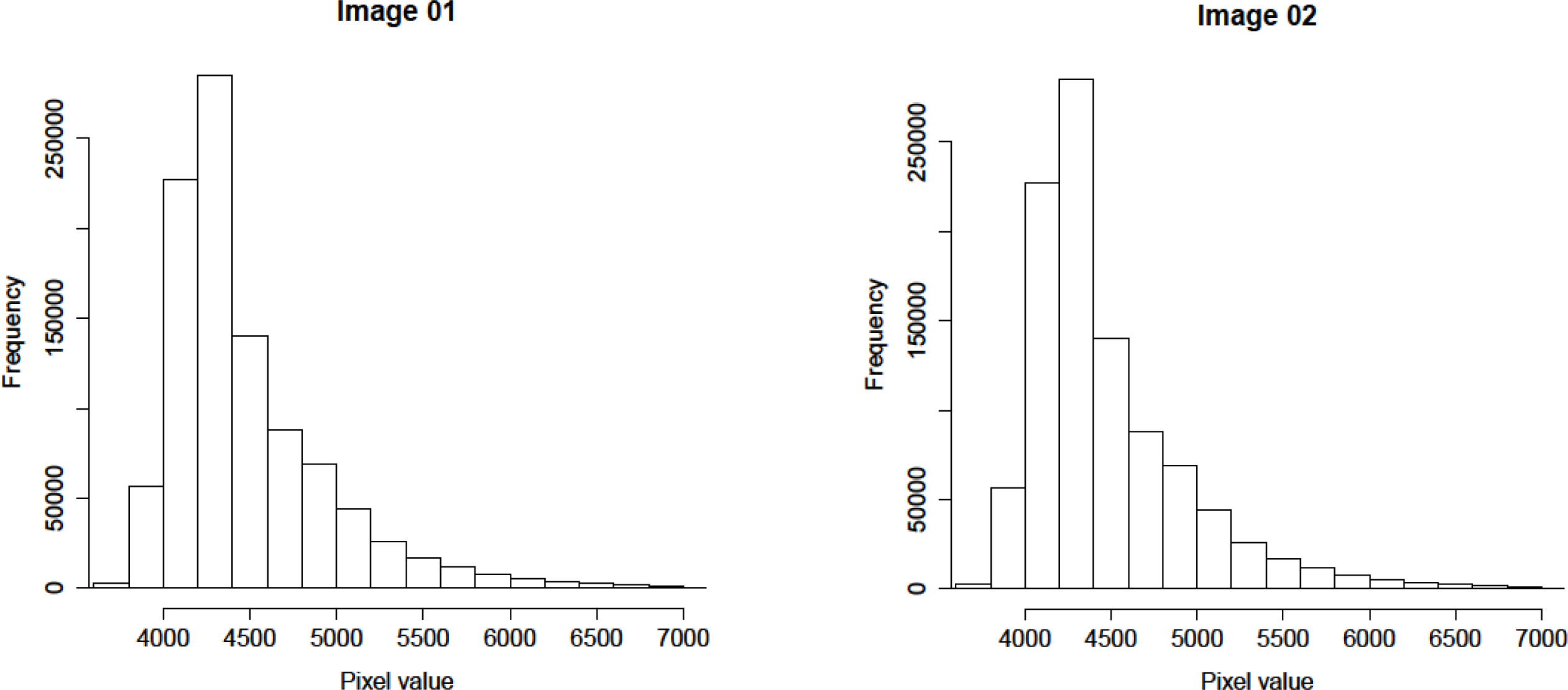
3.2. RapidEye Image Preprocessing

Before using the RapidEye images in the final calculation, the necessity of radiometric correction was examined according to the Ridge method [38]. The main idea is the linear relationship of the digital numbers (DNs) over pseudo-invariant features (PIFs) across these two images [39,40]. We made five feature space (for five RapidEye bands) images within these two images in the overlapping area. We used one band as the X axis and the same band in the other image as a Y axis to create the feature space image using the ERDAS IMAGINE software (version 10.1) and with the different colors representing histogram frequencies. We found that the slope and intercepts in the resulting feature space images (Figure 2a–e) were always one and zero, respectively. So, we determined that the radiometric correction was unnecessary. We also created the histograms and found a similar distribution in the overlapping area of these two images, which confirmed our previous results from the feature space images (e.g., blue band, Figure 3).

3.3. Estimation of RapidEye predictors

The spectral and textural features were calculated from the RapidEye images and used as predictors for modelling. The extraction was done based on the field plot size and RapidEye image pixel size so that the extracted image value could properly represent the forest attributes (e.g., AGB) at the plot level. The spectral predictors were derived from each band of RapidEye image by taking the mean DN values based on the plot size. Three spectral vegetation indexes were computed from the RapidEye images. Normalized Difference Vegetation Index (NDVI) (Equation (4)) is strongly related to the photo-synthetically active radiation intercepted by live vegetation, and is thus a robust method to identify live canopies in multispectral images [41]. NDVI has been widely used for estimating forest biomass [17]. NDVI is calculated from the visible (red) and near-infrared (NIR) bands of the RapidEye sensor (Equation (4));

$${\mathit{NDVI}}_{\mathit{1}}=(\mathit{NIR}-\mathit{Red})/(\mathit{NIR}+\mathit{Red})$$

(4)

NDVI thus varies between −1.0 and +1.0, i.e., green vegetation gives a positive value, snow and clouds tends to give negative values, whereas water and soil give values close to zero.

Also, the red-edge and green band ratio in the RapidEye images has a good response to forest biomass. Thus, the second NDVI [42] was calculated from these individual measurements (Equation (5)). In addition, the third NDVI [43] was calculated from the red-edge and red channel of the RapidEye image (Equation (6)) and is well-known as Normalized Difference Red Edge Index (NDRE). Given the sensitivity of the NDRE, this index is used for a variety of forest applications including biomass mapping and forest health.

$${\mathit{NDVI}}_{\mathit{2}}=(\mathit{Red}\hspace{0.17em}\mathit{edge}-\mathit{Green})/(\mathit{Red}\hspace{0.17em}\mathit{edge}+\mathit{Green})$$

(5)

$${\mathit{NDVI}}_{\mathit{3}}=(\mathit{Red}\hspace{0.17em}\mathit{edge}-\mathit{Red})/(\mathit{Red}\hspace{0.17em}\mathit{edge}+\mathit{Red})$$

(6)

We ran the Pearson correlation test to confirm which NDVI has the better correlation with AGB and volume. The Pearson correlation showed that the first NDVI and third NDVI had better correlations (r = −0.32 and −0.34, respectively) compared to the second NDVI (r = −0.12). A total of 14 textural features [24] were computed from the first and the third NDVI, separately.

The Haralick textural features were derived from the RapidEye images by considering the mean DNs based on the plot size. The co-occurrence matrix was used as an input to compute the Haralick’s features. We used single spectral bands (mean), three vegetation indices (e.g., normalized difference vegetation index) and Haralick textural features from RapidEye satellite data. Finally, a total of 36 RapidEye explanatory predictors (

Table 4. List of RapidEye explanatory predictors.

RapidEye Predictors	Description
B1	Blue (mean)
B2	Green (mean)
B3	Red (mean)
B4	Red-edge (mean)
B5	NIR (mean)
NDVI1	First NDVI (mean)
NDVI2	Second NDVI (mean)
NDVI3	Third NDVI (mean)
HR1	Angular second moment
HR2	Contrast
HR3	Correlation
HR4	Sum of squares
HR5	Inverse difference moment
HR6	Sum average
HR7	Sum variance
HR8	Sum entropy
HR9	Entropy
HR10	Difference variance
HR11	Difference entropy
HR12	Information measures of correlation
HR13	Information measures of correlation
HR14	Maximum correlation coefficient

) including both spectral and textural features were available for the prediction of the volume and AGB.

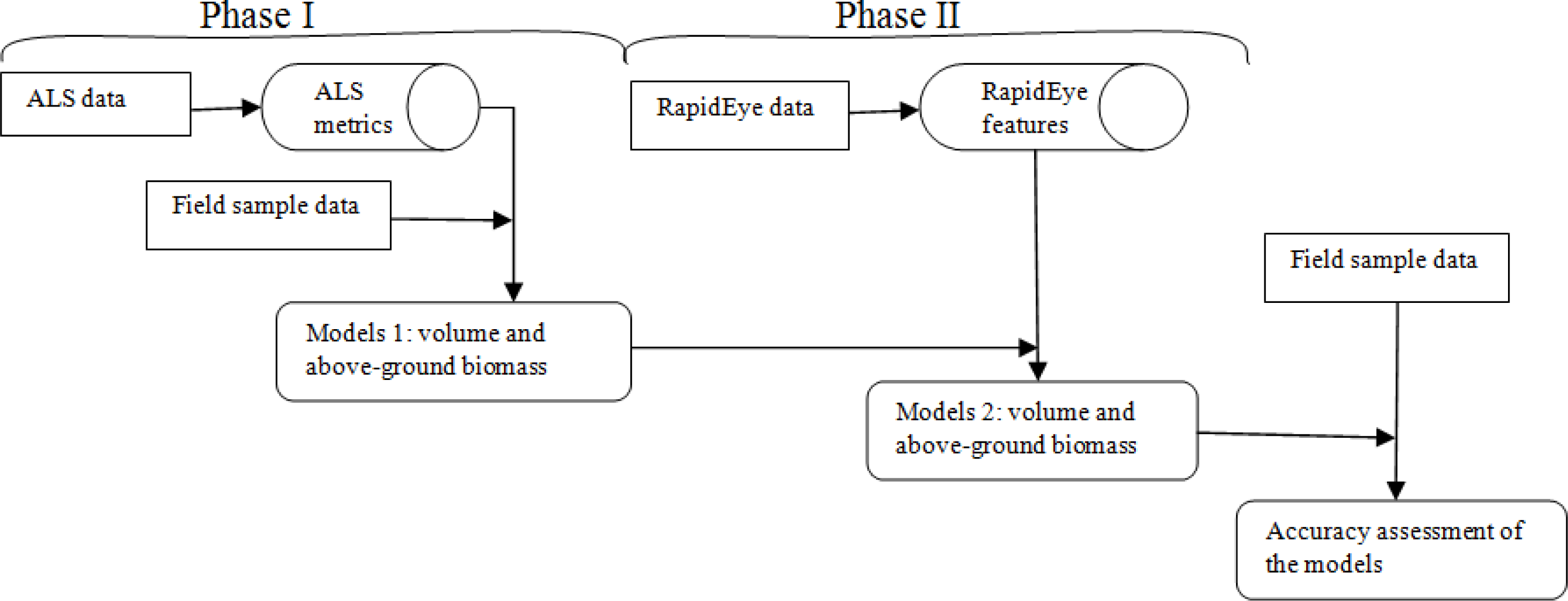
3.4. Two-Phase Sampling Method

Figure 4 shows the flowchart of the two-phase sampling method. In the first phase of this approach, a regression model is generated based on the relationship between ALS-metrics and field-measured sample plots. In the second phase, the forest characteristics that are estimated for the “surrogate plots” from ALS data are applied as simulated ground-truth to generate a regression model between forest parameters (e.g., AGB) and features derived from RapidEye satellite imagery.

3.5. Statistical Modeling

Ordinary least squares (OLS) is the most commonly employed method for estimating the unknown parameters of a linear regression model. The OLS can be written as follows in Equation (7);

$$Y_i=X_i^{\prime }\beta +{\epsilon }_i$$

(7)

where Y_i = field values of volume/AGB, β is a vector of regression coefficients; X′_i is a matrix of the explanatory variables from ALS data as well as from RapidEye data; ε_i is an unobserved error which account for the difference between the actually observed responses Y_i and the predicted values X′_iβ. We did not employ non-parametric method due to the insufficient number of training plots.

As we had a large number of predictors, we used the leaps package (regsubsets algorithm) in R (Version 2.15.2) environment to select the best combination of predictors for the models [44]. It performs an exhaustive search for the best subsets of the explanatory variables in X for predicting Y (dependent variable) in linear regression, using an efficient branch-and-bound algorithm. The selection criteria in the algorithm were Bayesian Information Criterion (BIC) and adjusted R² (coefficient of determination) value. Since the algorithm returns the best model of each size (number of predictors), the results do not depend on a penalty model for model size. In addition to stepwise variable selection, we used the Pearson correlation techniques and the maximum R² improvement variable selection techniques to select ALS/RapidEye-derived variables to be included in the models. During the variable selection, no explanatory variable was left in the models with a partial F statistic with a significance level greater than 0.05. It is worth noting that regsubsets algorithms might have many independent variables that could introduce multicollinearity problems, i.e., one independent variable is a linear combination of the other independent variables. The problem is that, as the independent variables (e.g., ALS height percentiles) become more highly correlated to the dependent variables (e.g., AGB), it becomes more and more difficult to determine which independent variable is actually producing the effect on the dependent variables. In this circumstance, we used maximum R² improvement techniques to search for the “best” one-variable model, the “best” two-variable model, and so forth, although it is not guaranteed that in finds the model with the highest R² for each size. We repeated the selection 10 times by randomly selecting 50% of the observations for each repetition to produce stable models for our final regression models. Our final models contained the most frequently occurring ALS/RapidEye-derived variables. Næsset et al. [45] and Latifi et al. [46] used similar predictor selection techniques for model building to predict forest biomass and volume.

3.6. Model Accuracy Assessment

The RMSE and relative RMSE (Equation (8)) have been widely used for validating the accuracy of forest parameters estimation. The accuracy of fitted models was measured by using leave-one-out validation (LOOV) techniques. Bias is the mean residual error between predicted and estimated model values (Equation (9)). Relative bias gives the percentage of mean residual error (Equation (9)).

$$\mathit{RMSE}=\sqrt{\frac{{\sum }_{i=1}^n{(y_i-{\widehat{y}}_i)}^2}{\text{n}}};{\mathit{RMSE}}_{\%}=100\times \frac{\text{RMSE}}{\overline{y}}$$

(8)

$$\mathit{Bias}=\frac{{\sum }_{i=1}^n(y_i-{\widehat{y}}_i)}{n};\hspace{0.17em}\hspace{0.17em}{\mathit{Bias}}_{\%}=100\times \frac{\text{bias}}{\overline{y}}$$

(9)

where y_i is the predicted value for sample plot i; ŷ_i is the observed value for sample plot i; ȳ is the average value of measured sample plots, and n is the total number of plots. The statistical significance of the bias was estimated by the t-test (Equation (10)).

$$t=\frac{\mathit{Bias}}{\raisebox{1ex}{$\mathrm{SD}$}\!\left/ \!\raisebox{-1ex}{$\sqrt{n}$}\right.}$$

(10)

where SD is the standard deviation of the residuals (y − ŷ_i). The bias was considered to be significant if the absolute value of the t was greater than t corresponding with a probability of 0.05 [47]. The coefficients of determination (R² and adjusted R²) describe the model fit. A higher adjusted R² indicates a better model. The equation of adjusted R² is following (Equation (11));

$$R^2\mathit{adjusted}=1-(1-R^2)\frac{(n-1)}{n-k-1}$$

(11)

where, n is the sample size and k is total number of regressors in the linear model (not counting the constant term).

4. Results

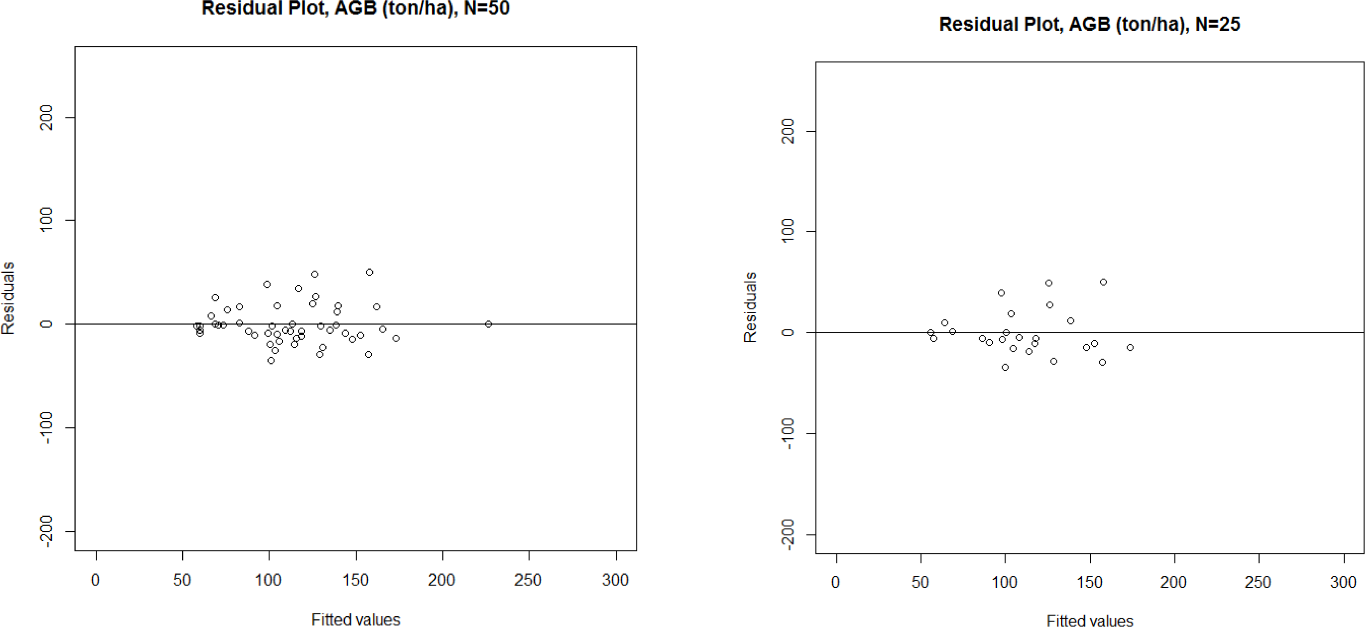
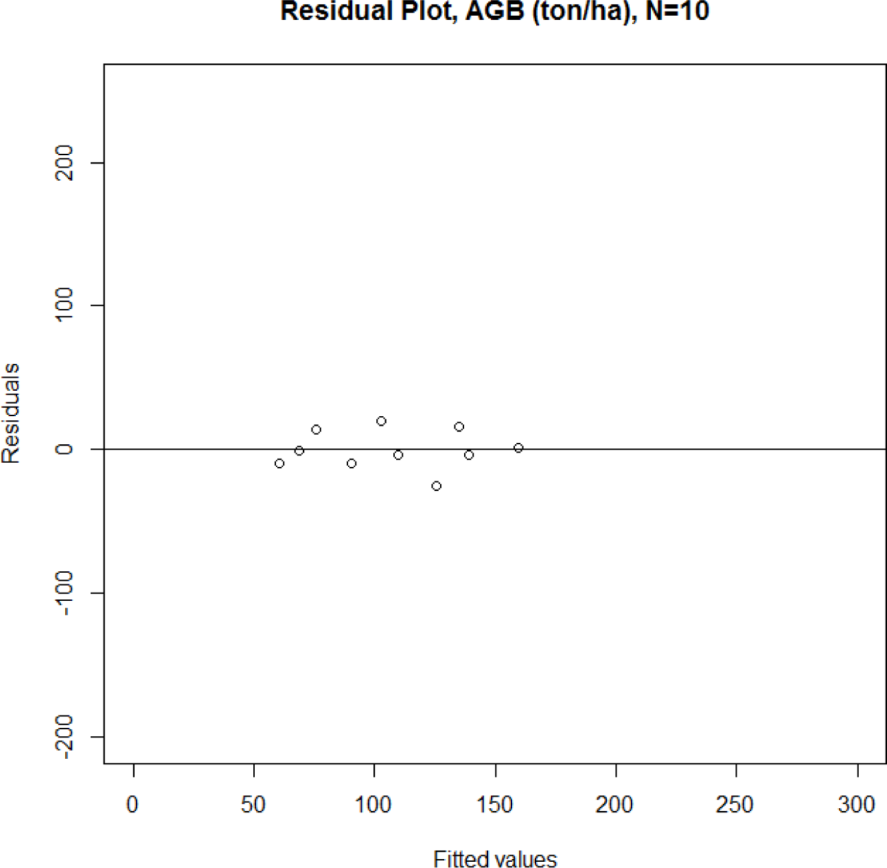
4.1. Model Building and Accuracy at Phase I (ALS data)

The precisions of the ALS models are detailed in

Table 5. Accuracy of the ALS prediction against field estimation.

Parameter	Number of Training Plots (n)	Mean of Estimates	Standard Deviation of Estimates	RMSE	RMSE %	Bias	Bias %	R2 Adj.
AGB *, ton/ha	50	112.9	34.8	18.7	16.6	0.0	0.0	76.6
Volume, m3/ha		209.2	66.2	34.5	16.5	0.0	0.0	77.7
AGB *, ton/ha	25	111.5	31.9	22.0	19.7	0.0	0.0	65.3
Volume, m3/ha		204.1	56.2	41.7	20.4	0.0	0.0	61.9
AGB *, ton/ha	10	106.6	32.9	13.0	12.2	0.0	0.0	83.2
Volume, m3/ha		198.8	67.7	25.1	12.6	0.0	0.0	85.0

^{AGB *:}above ground biomass. R² Adj: R² adjusted.

. Table A1 shows the model parameters and their statistical significance. Scatter plots are presented in Figure 5 to illustrate the residual plots for AGB. Although, we had a total of 46 ALS predictors initially in the set, the final AGB and volume models include only one ALS predictor. We also tested the transformation of the ALS predictors instead of the original value but it did not improve our model accuracy. The ratio of last and single echoes with height lower than 13.5 m and the total number of last and single echoes constituted the best model for AGB and volume.

Table 5 shows the accuracy of the ALS prediction against field estimation using three combinations of training plots (50, 25 and 10 training plots). We reduced the number of training plots from 50 to 25 and 10 training plots (phase I) to assess the prediction accuracy after reducing the number of training plots. After sorting the training plots based on the tree height and AGB distribution, we selected every second plot to obtain 25 training plots, and every fifth plot to obtain 10 training plots out of 50 plots. The results in Table 5 proved that the models based on all three combinations of training plots had promising prediction accuracy. The linear model that was calibrated to estimate AGB showed high correlation when validated against field estimation using LOOV. A lowest RMSE value of 13 tons/ha (12%) was observed for AGB, while volume had similar RMSE value of 25 m³/ha (12%) for the models based on 10 training plots. In contrary, the highest 20% RMSE of AGB was employed for the models based on 25 training plots. In addition, the R² of the model was 0.83 based on 10 training plots. A slightly better R² value (0.85) was observed for volume. However, the models based on 25 training plots had a lowest R² value for both AGB (0.65) and volume (0.61). The statistical outliers were not frequent in the each residual plot (Figure 5). Although our final AGB and volume models each contain one ALS predictor, tests were also conducted by adding more ALS height and density predictors to the models. However, this did not improve the model accuracy significantly. For instance, we added the 80% ALS height percentile in the AGB model in addition to the used ALS predictor. However, the R² value dropped from 0.83 to 0.50. Similarly, we added the ratio of the number of last and single echoes below 5 m (low vegetation) and the total number of last and single echoes in the AGB model. Similarly, the R² value dropped to 0.66. Besides, the Pearson correlation between the used density metric and tree AGB, volume, tree height, basal area were respectively 0.84, 0.85, 0.82, 0.75, which confirms that this density metric explained very well the structure of study area. In contrast, the correlations between the ALS height percentiles of 60%, 70%, 80%, 90% and AGB were 0.60, 0.61, 0.62, and 0.64, respectively. In the case of volume, the correlations were higher for the ALS height percentiles and were respectively 0.68, 0.68, 0.69 and 0.70, which indicates that the ALS height percentiles correlate better with volume than AGB. The key of the used density metric must be the 13.5 m height threshold; it is much higher than what is typically used. 13.5 m seems to be close to the smallest mean height at the plots. We think that it is a combination of a small variation in the plot data and the unusually high threshold which somehow makes this variable special for this particular data set. It might also be possible to achieve these results in a managed commercial forest, where an increase in height would also result in an increase in density, so one density variable would be enough.

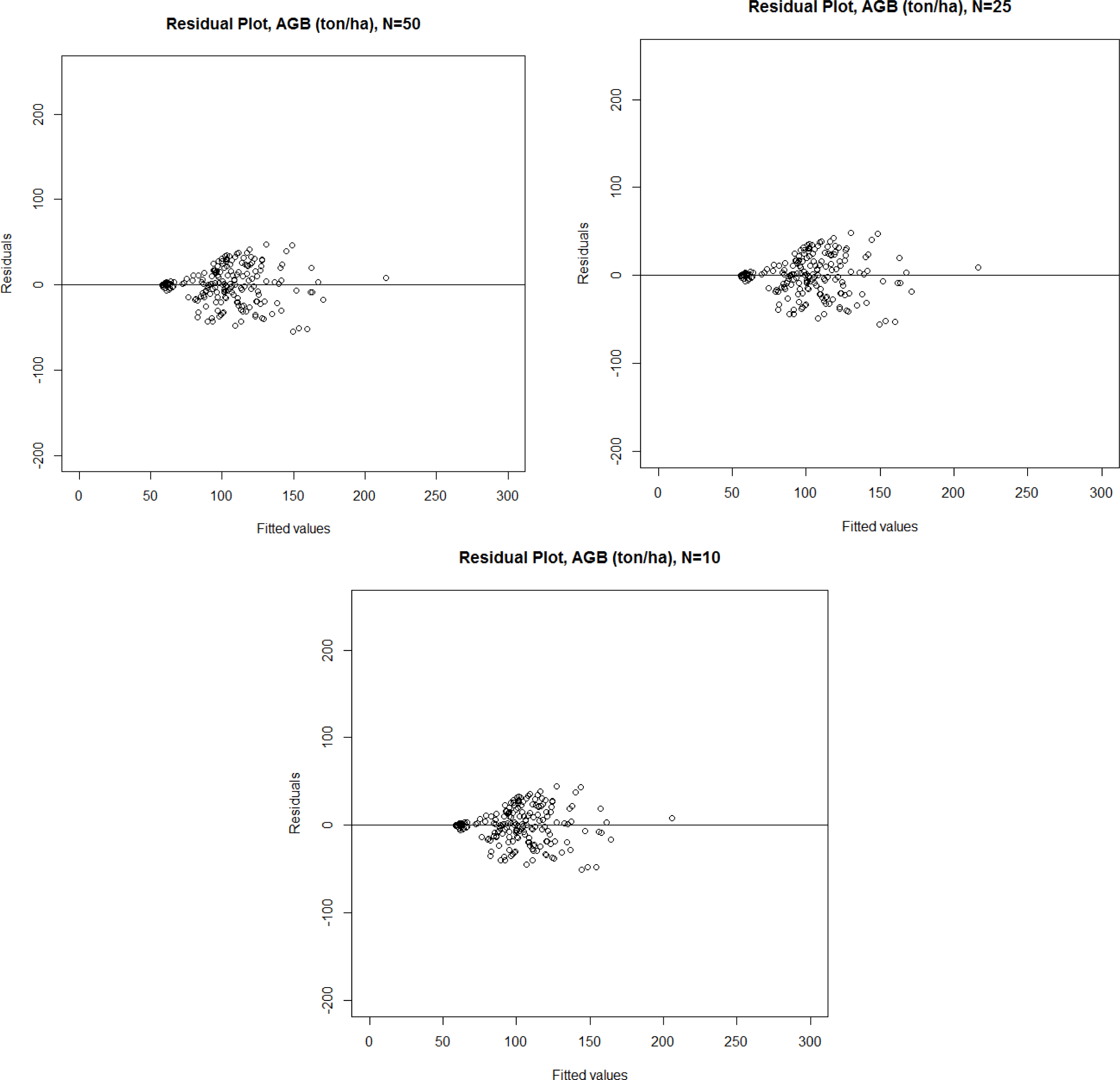
4.2. Model Building and Accuracy at Phase II (RapidEye Data)

The error statistics of the linear models are given in

Table 6. Accuracy of RapidEye prediction against ALS estimation at phase II.

Parameter	Number of Training Plots (n) ǂ	Number of Surrogate Plots	Mean of Estimates	Standard Deviation of Estimates	RMSE	RMSE %	Bias	Bias %	R2 Adj.
AGB *, ton/ha	50	200	102.7	26.2	21.0	20.4	0.0	0.0	59.5
Volume, m3/ha			189.7	49.3	40.6	21.3	0.0	0.0	58.4
AGB *, ton/ha	25		101.4	26.8	21.5	21.2	0.0	0.0	59.5
Volume, m3/ha			186.3	46.8	38.5	20.6	0.0	0.0	58.4
AGB *, ton/ha	10		100.8	24.5	19.6	19.5	0.0	0.0	59.5
Volume, m3/ha			186.8	49.9	41.0	21.9	0.0	0.0	58.4

^{AGB *:}above ground biomass;

^ǂThe number of training plots from phase I used in the estimation of 200 ALS surrogate plots for phase II. R² Adj: R² adjusted.

. Table A1 shows the details of the regression models for RapidEye data. Figure 6 shows the residual plots for AGB. The predictor selection techniques picked up six and five predictors, respectively, for AGB and volume from a set of 36 independent RapidEye predictors. The best model for AGB constitute with the mean of four RapidEye spectral bands (green, red, red-edge, NIR), mean NDVI (based on red-edge and green) and the Haralick feature of inverse difference moment (HR5). Volume model consist of all AGB predictors except red band (mean). The mean NDVI and inverse difference moment accounted for much more of the variability in biomass and volume than the individual RapidEye bands. Notably, the RapidEye spectral bands were very helpful in increasing the variance explained.

We calibrated the RapidEye models against ALS-trained set of surrogate plots using LOOV. The mean and standard deviation of AGB for the ALS-trained set of surrogate plots were 103 tons/ha and 34 tons/ha, respectively. We had a similar accuracy for all the combination of training plots number (10, 25, and 50). However, RapidEye prediction based on the 10 training plots against ALS estimation gave a lowest RMSE of 19 tons/ha (19%) for AGB. In addition, volume had a similar RMSE 38–41 m³/ha (20%–21%) value from all the combination of training plots (Table 6). The RapidEye predicted value showed a high correlation against the ALS estimates. The model for AGB explained 59% of the variability whereas the model for volume explained 58% (Table 6). The RapidEye model was not affected by the saturation effect (suppression of variance). Albeit, the AGB model did not show any heteroscedasticity in the model, the volume model had some affect but was not statistically significant. We used the logarithmic and quadratic transformation in an attempt to minimize this problem but they did not improve the model significantly.

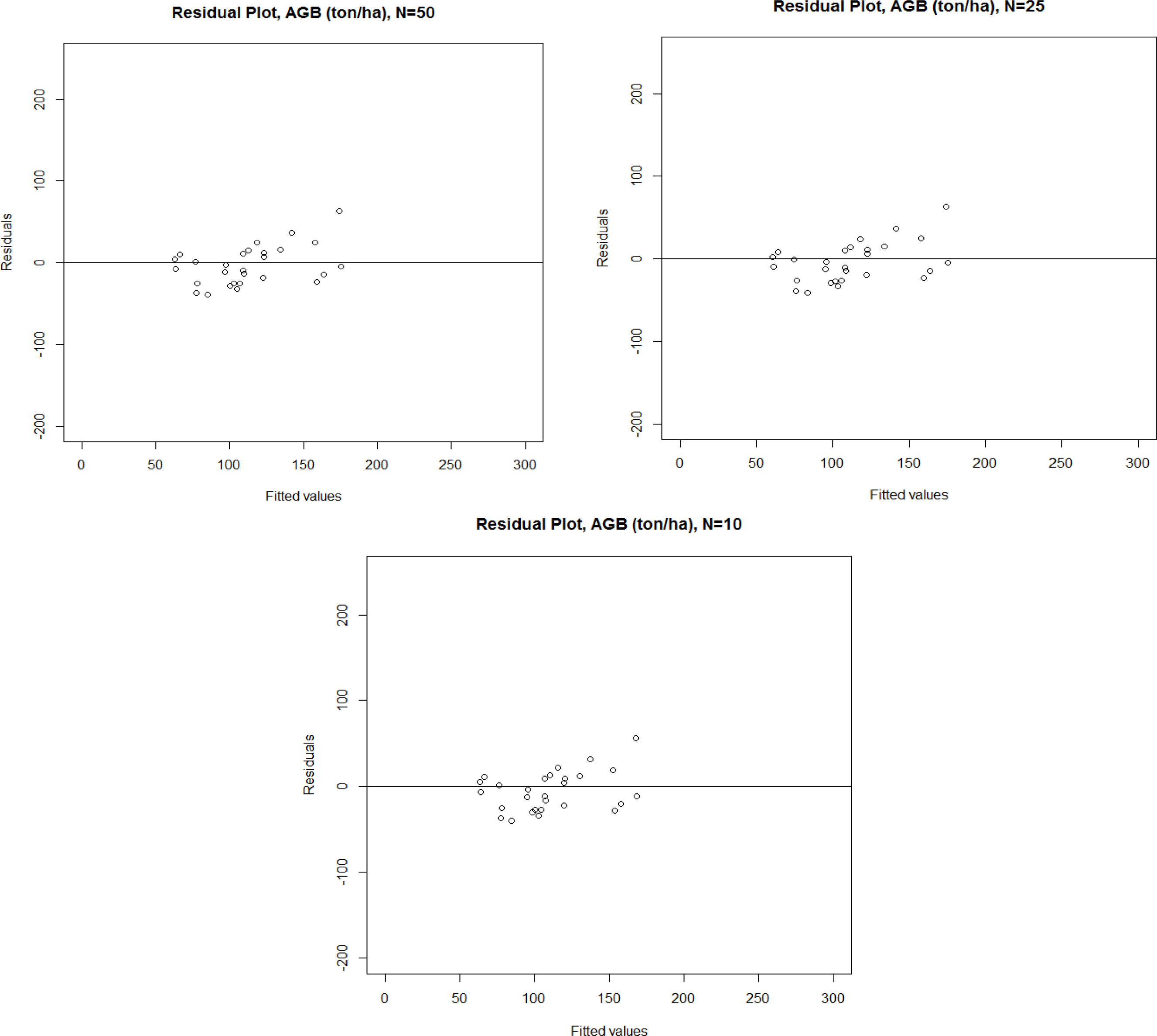
4.3. Accuracy at the Independent Validation Plots

The accuracies at the validation plots are shown in

Table 7. Accuracy of AGB and volume obtained from RapidEye at validation plots.

Parameter	Number of Training Plots (n) ǂ	Number of Validation Plots (n)	Mean of Estimates	Standard Deviation of Estimates	RMSE	RMSE %	Bias	Bias %	R2 Adj.
AGB *, ton/ha	50	28	112.5	32.5	23.6	20.4	−3.1	−2.7	50.7
Volume, m3/ha			207.5	59.4	43.2	19.7	−11.4	−5.2	54.0
AGB *, ton/ha	25		111.5	33.3	24.1	20.8	−4.1	−3.5	50.7
Volume, m3/ha			203.2	56.4	44.3	20.2	−15.7	−7.1	54.0
AGB *, ton/ha	10		110.0	30.4	23.3	20.2	−5.6	−4.8	50.7
Volume, m3/ha			204.9	60.1	44.3	20.1	−14.1	−6.4	54.0

^{AGB *:}above ground biomass;

^ǂThe number of training plots used in the estimation of 200 ALS surrogate plots at phase II. R² Adj: R² adjusted.

. Figure 7 shows the residual plots comparing the RapidEye prediction against field estimation for AGB. The residual plots for AGB are reasonably good (Figure 7) despite a slight non-linearity in the case of volume. Table 7 shows that there was relatively similar accuracy for the validation plots using three combinations of training plots. However, the models based on the 10 training plots had slightly better accuracy for AGB, while volume prediction accuracy was highest in the models based on 50 training plots. A RMSE value of 23–24 tons/ha (20%) was observed AGB, while volume had a RMSE value of 43–44 m³/ha (19%–20%). We found that these accuracies at the independent validation plots can be considered acceptable and are even better than in studies concerning conventional compartments-based field inventory in Finland [48,49]. All the biases were insignificant at the independent validation plots. It is worth noting that due to the small number of independent validation plots (n = 28), the imprecision in terms of the relative bias is no longer observed when predictions are plotted versus measured observations because the absolute scatter is approximately the same. In contrast, we also fitted the RapidEye model directly using 50 field plots, and used it to predict 28 validation plots. We found that the accuracy was slightly lower compared to the prediction with the use of surrogate plots (phase II). The relative RMSE and the adjusted R² were 21% and 44%, respectively, for AGB.

5. Discussion and Conclusion

This paper presented and tested forest AGB and volume estimation using ALS and RapidEye sensor data in a mixed-species boreal forest of eastern Finland. We found that the outcomes of the study were encouraging and we felt that they need further validation in other forest types along with development of the methodology. The overall strength of the ALS–RapidEye fusion revealed here is a promising accuracy to characterize biomass accounting in the coniferous forest ecosystems. The analysis of linear regression showed that the ALS data had good prediction accuracy at phase I. It was promising that the ALS models explained 83% (R² value of 83%) of the variability for AGB. Furthermore, the RapidEye models provided a relatively good accuracy at phase II for AGB and as well as for volume. RapidEye data had a relative RMSE of 20% at independent validation plots. Such accuracy indicates that the combination of ALS and RapidEye would be a promising fusion for the estimation of boreal forest attributes. Nevertheless, more testing and validation should be done in different forest landscapes at large-scale.

5.1. Statistical Modelling

We used the simple linear regression to predict biomass and volume which is one of the most commonly used methods in remote sensing-based regression modeling (e.g., [17,50–52]). Næsset et al. [53] made a conclusion that employing a multivariate (multi-variable) method would not have had any significant impact on the biomass and volume estimation among the tested OLS regression analysis, seemingly unrelated regression (SUR), and partial least-squares (PLS) regression from two different inventories using ALS data.

Though we used regression subset selection techniques (leaps package) using an efficient branch-and-bound algorithm in R statistics, Packalén et al. [54] mentioned that different predictor variables were identified during different runs of the automated variable selection method. For instance, Latifi et al. [46], Packalén et al. [55] reported that genetic algorithm (GA) and simulated annealing (SA) were also superior variable selection methods. These algorithms should nevertheless be tested as alternatives to see whether a different explanatory variable selection method would improve the result or at least make the search for an eventual solution more effective. Nevertheless, the ALS predictor (density metric) that we employed in the biomass and volume models was closely matched to the predictors selected in other studies (e.g., Rana [56]). The RapidEye spectral and textural features used in this study are also closely matched with other studies (e.g., Packalén et al. [26] and Latifi et al. [46]).

5.2. Method Pros and Cons

Our presented forest biomass inventory method naturally places some advantages and constraints on the applicability of the method. Albeit, it involves a sample ALS data at phase I and requires only a few sample plots for model calibration (fitting). In addition, the surrogate plots (phase II) could be placed systematically in the whole area based on vegetation types, geographic location, climatic condition and tree species compositions. Therefore, our calibrated models at phase II represent the whole study area and have less chance of missing the vegetation types and tree species’ compositions. The surrogate plots should be placed so that they reflect the full range of variation in biomass over the study area. In addition, the surrogate plots should cover also the rare forest types. Systematic selection or selection based on predicted AGB would be a natural choice. The locations of the surrogate plots could be selected through weighted random sampling or stratified sampling. Traditional forest inventory depends on a large set of ground-truth data for model calibration. However, this study showed a promising outcome where a sample ALS data was employed as a ground-truth data for model calibration with the satellite image for mapping the whole area of interest.

Another issue is that the satellite image acquisition dates may be different, introducing seasonal effects. Therefore, it would require the DN (digital number) values to be comparable between datasets which in turn would require the use of absolute reflectance instead of relative DN values. It would be recommended to use the same season for image acquisition. The result from Figures 2 and 3 confirmed that we did not need image normalization here. However, image normalization would be required for all satellite images relative to each other. In addition, the field data should always be collected at the same time period/season. In our study, the RapidEye images were collected almost two years after the field and ALS data acquisitions. However, it is acceptable in our study because there was no harvesting and logging activities and no significant naturally occurring changes within that time period.

Our study showed that ALS-based forest inventory have produced very accurate estimates (phase I). ALS data have high accuracy to predict forest biomass when regressing ALS height/density metrics with data from field measured plots [57]. Subsequently, ALS estimates for the surrogate plots were used as simulated ground-truth (phase II) for the interpretation of optical satellite images, which improved the results compared with using models that were directly based on the field plots. Covering the whole area of interest with ALS is relatively expensive, thus we used a two-phase estimation approach that requires ALS data only from a sample of the study area. This is known as the ALS-assisted multi-source programme that combines ALS information with field plots and satellite data to develop a forest biomass map [58].

Reducing the number of training plots is of great importance to minimize field inventory cost. Our findings show that a reduced number of sample plots provides similar accuracy compared to the full dataset. When we reduced the sample plot from 50 to 10, there was no significant reduction in the prediction accuracy of AGB and volume (Table 7). Junttila et al. [59] reported similar performances in the boreal managed forest area, Finland. They concluded that the effect of a reduction in sample-plot number had only a slight decrease in accuracy and a reduction of 2.9% RMSE for the reduced sample-plot number compared to the full dataset. Latifi and Koch [60] thoroughly studied the integration of off-site samples into small-scale forest inventory in central Europe, in which they reported the substantial effectiveness of low-to-medium sampling intensity on improving forest structure models by means of ALS and multispectral aerial images. Dalponte et al. [61] concluded that it is possible to reduce the number of field sample plots without losing model accuracy. A bottleneck of their approach was that ALS data is necessary as prior information before collection of field reference data. They reduced the number of sample plots based on genetic algorithms, whereas our selections were based on tree height and AGB distribution.

5.3. Model Calibration and Validation

The ALS models were calibrated against the field sample plots in phase I of the model building. The R² value of our predicted forest AGB is close to the others studies ranged between 0.74 and 0.88 in the studies by Hall et al. [62], Bright et al. [63], Fu et al. [64], Gobakken et al. [65], Næsset and Gobakken [45], Hawbaker et al. [66] and Ferster et al. [67]. Subsequently, in the phase II, we calibrated the RapidEye models against the ALS-simulated estimation. When the resulting models at phase II were tested against an independent dataset, the error statistics of testing were similar to those of the model fitting (Tables 6 and 7). Our models are stable and more promising considering the error statistics. Næsset [68], Gómez et al. [69], Eckert [70], and Gautam [22] mentioned that optical imagery based estimation may lead to significant underestimation of biomass stock in areas with high (>200 ton/ha) AGB concentrations. In western Finland, Muukkonen and Heiskanen [71] had faced a similar problem in mixed special boreal forest employing optical sensor alone where biomass was underestimated above 200 ton/ha. Our models and vegetation index were not affected by the saturation problem (underestimation of variance) because the biomass stock at the study area is mostly less than 200 ton/ha, although many authors have reported this problem for optical sensors. However, it would be interesting to explore the accuracy of our presented approach in other landscapes for wider acceptance based on the geographic variation and different forest types and environments.

The RMSE at the independent validation plots was lower than in most previous studies of boreal coniferous and mixed forest. Our study had a relative RMSE of 19%–20% for volume, whereas previous studies using the optical sensor had a relative RMSE of 42%–82% for volume, for instance, studies by Tokola and Heikkilä [72] (82%), Tomppo et al. [73] (59%), Kilpeläinen and Tokola [74] (56%), Hyyppä et al. [75] (50%), Mäkelä and Pekkarinen [76] (47%), and Hyvönen [77] (42%). Similar to the volume, the relative RMSE (20%) for AGB was also noticeably lower in the present study than the corresponding statistics of Tomppo et al. [73] (36%), and Muukkonen and Heiskanen [71] (41%). It is worth noting that the above studies did not follow exactly the same approach of our study but are the closest available comparison. The biases were considerably higher for testing datasets compared to the model fitting, though the biases were not statistically significant. Due to the small number of testing plots we could not make a clear conclusion about biases here.

5.4. Sensor Pros and Cons

The relatively small errors in this study are probably due to the type of biomass being measured and the relatively good spatial and spectral resolution of the RapidEye data with high geometric accuracy. Hyyppä et al. [75] also mentioned that the estimation error of the forest characteristics were smaller for higher resolution data compared to the lower resolution data. Good spatial resolution of the RapidEye bands makes it is a good data source for studies of forest characteristics. Koch [78], Treitz et al. [79], and Kankare et al. [80] mentioned that the mapping of forests biomass, from local to global in terms of their status and development, is of increasing importance for REDD.

5.5. Concluding Remarks

We examined here the AGB and volume estimation employing ALS and RapidEye data in a two-phase sampling method. Linear regression was employed to predict forest characteristics in a managed boreal forest in eastern Finland. To conclude, the present study has confirmed that the accuracy of AGB and volume comparable to the forest inventory by compartments (or stand) in Finland. The approach presented here is a promising alternative for use in forest management in Finland with enough accuracy for the purpose of forest resource inventory. In addition, calibrating the RapidEye data using the ALS-simulated surrogate plots and different models at phases I and II make this approach promising and stable for biomass and carbon accounting in the boreal forest. It could also offer valuable methodology for inventories need in the REDD program. As the tested area is rather small, further validation is needed in a larger study area for better justification of the presented approach. Finally, we feel that future studies should be carried out using a combination of ALS and other optical sensors to confirm the validity of this approach in other forests landscape. This approach could be tested by tracking changes in forest biomass at the regional and national levels.

References

1. Winjum, J.K.; Dixon, R.K.; Schroeder, P.E. Forest management and carbon storage: An analysis of 12 key forest nations. Water Air Soil Pollut 1993, 70, 239–257. [Google Scholar]
2. United Nations Framework Convention on Climate Change (UNFCCC). Kyoto Protocol Reference Manual on Accounting of Emissions and Assigned Amounts. Available online: http://unfccc.int/files/national_reports/accounting_reporting_and_review_under_the_kyoto_protocol/application/pdf/rm_final.pdf (accessed on 10 June 2013).
3. Rosenqvist, A.; Milne, A.; Lucas, R.; Imhoff, M.; Dobson, C. A review of remote sensing technology in support of the Kyoto protocol. Environ. Sci. Policy 2003, 6, 441–455. [Google Scholar]
4. Intergovernmental Panel on Climate Change (IPCC). Good Practice Guidance for Land Use, Land-Use Change and Forestry; IPCC National Greenhouse Gas Inventories Programme: Hayama, Japan, 2003. [Google Scholar]
5. Streck, C.; Scholz, S.M. The role of forests in global climate change: Whence we come and where we go. Int. Aff 2006, 82, 861–879. [Google Scholar]
6. Southworth, J.; Gibbes, C. Digital remote sensing within the field of land change science: Past, present and future directions. Geogr. Compass 2010, 4, 1695–1712. [Google Scholar]
7. Houghton, R.A. Aboveground forest biomass and the global carbon balance. Glob. Chang. Biol 2005, 11, 945–958. [Google Scholar]
8. Saatchi, S.; Houghton, R.A.; Dos-Santos-Alvala, R.C.; Soares, J.V.; Yu, Y. Distribution of aboveground live biomass in the Amazon basin. Glob. Chang. Biol 2007, 13, 816–837. [Google Scholar]
9. Global Observation of Forest and Land Cover Dynamics (GOFC-GOLD). Reducing Greenhouse Gas Emissions from Deforestation and Degradation in Developing Countries: A Sourcebook of Methods and Procedures for Monitoring, Measuring and Reporting; GOFC-GOLD Report Version COP14-2; GOFC-GOLD Project Office, Natural Resources Canada: Edmonton, AB, Canada, 2009. [Google Scholar]
10. Wilkie, M.L. Global Forest Resource Assessment Report, Finland; FRA Report No. 69; FAO Forestry Department VialedelleTerme di Caracalla: Rome, Italy, 2010. [Google Scholar]
11. Myneni, R.B.; Keeling, C.D.; Tucker, C.J.; Asrar, G.; Nemani, R.R. Increased plant growth in the northern high latitudes from 1981 to 1991. Nature 1997, 386, 698–702. [Google Scholar]
12. Hame, T.; Salli, A.; Andersson, K.; Lohi, A. A new methodology for the estimation of biomass of conifer dominated boreal forest using NOAA AVHRR data. Int. J. Remote Sens 1997, 18, 3211–3243. [Google Scholar]
13. Kauppi, P.E.; Mielikäinen, K.; Kuusela, K. Biomass and carbon budget of European forests, 1971 to 1990. Science 1992, 256, 70–74. [Google Scholar]
14. Næsset, E.; Gobakken, T.; Holmgren, J.; Hyyppä, H.; Hyyppä, J.; Maltamo, M.; Nilsson, M.; Olsson, H.K.; Persson, Å S.; Derman, U.S. US Laser scanning of forest resources: The Nordic experience. Scand. J. For. Res 2004, 19, 482–499. [Google Scholar]
15. Drake, J.B.; Knox, R.G.; Dubayah, R.O.; Clark, D.B.; Condit, R.; Blair, J.B.; Hofton, M. Above-ground biomass estimation in closed canopy neotropical forests using ALS remote sensing: Factors affecting the generality of relationships. Glob. Ecol. Biogeogr 2003, 12, 147–159. [Google Scholar]
16. Asner, G.P.; Hughes, R.F.; Varga, T.A.; Knapp, D.E.; Kennedy-Bowdoin, T. Environmental and biotic controls over aboveground biomass throughout a rain forest. Ecosystems 2009, 12, 261–278. [Google Scholar]
17. Hou, Z.; Xu, Q.; Tokola, T. Use of ALS, Airborne CIR and ALOS AVNIR-2 data for estimating tropical forest attributes in Lao PDR. ISPRS J. Photogramm. Remote Sens 2011, 66, 776–786. [Google Scholar]
18. Maltamo, M.; Bollandäs, O.M.; Næsset, E.; Gobakken, T.; Packalén, P. Different plot selection strategies for field training data in ALS-assisted forest inventory. Forestry 2011, 84, 23–31. [Google Scholar]
19. Watt, P.; Watt, M. Applying satellite imagery for forest planning. NZ J. For 2011, 56, 23–25. [Google Scholar]
20. Ozdemir, I.; Ozkan, K.; Mert, A.; Ozkan, U.Y.; Senturk, O.; Alkan, O. Mapping Forest Stand Structural Diversity Using Rapideye Satellite Data. Available online: http://congrexprojects.com/docs/12c04_docs2/poster2_6_ozdemir.pdf (accessed on 11 December 2012).
21. Garcia, M.; Riano, R.; Chuvieco, E.; Danson, F.M. Estimating biomass carbon stocks for a Mediterranean forest in central Spain using LiDAR height and intensity data. Remote Sens. Environ 2010, 114, 816–830. [Google Scholar]
22. Gautam, B.R. LiDAR-Assisted Multi-source Program (LAMP) for FRA Nepal; FRA Bulletin No. 1; MoFSC/Department of Forest Research and Survey: Kathmandu, Nepal, 2011. [Google Scholar]
23. Tamura, H.; Mori, S.; Yamawaki, T. Textural features corresponding to visual perception. IEEE Trans. Syst. Man Cybern 1978, 8, 460–472. [Google Scholar]
24. Haralick, M.R.; Shanmugam, K.; Dinstein, J. Textural features for image classification. IEEE Trans. Syst. Man Cybern 1973, 3, 610–621. [Google Scholar]
25. Tuominen, S.; Pekkarinen, A. Performance of different spectral and textural aerial photograph features in multi-source forest inventory. Remote Sens. Environ 2005, 94, 256–268. [Google Scholar]
26. Packalén, P.; Maltamo, M. The k-MSN method for the prediction of species specific stand attributes using airborne laser scanning and aerial photographs. Remote Sens. Environ 2007, 109, 328–341. [Google Scholar]
27. Holopainen, M.; Talvitie, M. Forest inventory by means of tree-wise 3D-measurements of laser scanning data and digital aerial photographs. Int. Arch. Photogramm. Remote Sens. Spat. Inf. Sci 2012, XXXVI-8/W2, 67–72. [Google Scholar]
28. Tegel, K. A Comparison of Landsat-7 ETM+ and Terrasar-X Satellite Imagery in Estimating Forest Aboveground Biomass in a Two-Stage Sampling Procedure. M.Sc. Dissertation,. University of Helsinki: Helsinki, Finland, 2011. [Google Scholar]
29. Gautam, B.; Peuhkurinen, J.; Kauranne, T.; Gunia, K.; Tegel, K.; Latva-Käyrä, P.; Rana, P.; Eivazi, A.; Kolesnikov, A.; Hämäläinen, J.; et al. Estimation of Forest Carbon Using LiDAR-Assisted Multi-Source Programme (LAMP) in Nepal. Proceedings of the International Conference on Advanced Geospatial Technologies for Sustainable Environment and Culture, Pokhara, Nepal, 12–13 September 2013.
30. Laasasenaho, J. Taper curve and volume function for pine, spruce and birch. Commun. Instituti. For. Fenn 1982, 108, 1–74. [Google Scholar]
31. Repola, J. Biomass equations for scots pine and norway spruce in Finland. Silva. Fenn 2009, 43, 625–647. [Google Scholar]
32. Repola, J. Biomass equations for birch in Finland. Silva. Fenn 2008, 42, 605–624. [Google Scholar]
33. RapidEye. RapidEye—Delivering the World. Available online: http://www.rapideye.de (accessed on 1 February 2013).
34. Axelsson, P. DEM Generation from Laser Scanner Data Using Adaptive TIN Models. Proceedings of the XIXth ISPRS Conference, IAPRS, Amsterdam, The Netherlands, 16–22 July 2000.
35. Næsset, E. Practical large-scale forest stand inventory using small-footprint airborne scanning laser. Scand. J. For. Res 2004, 19, 164–179. [Google Scholar]
36. Junttila, V.; Kauranne, T.; Leppanen, V. Estimation of forest stand parameters from airborne laser scanning using calibrated plot databases. For. Sci 2010, 56, 257–270. [Google Scholar]
37. Næsset, E. Predicting forest stand characteristics with airborne scanning laser using a practical two-stage procedure and field data. Remote Sens. Environ 2002, 80, 88–99. [Google Scholar]
38. Song, C.; Woodcock, C.E.; Seto, K.C.; Lenney, M.P.; Macomber, S.A. Classification and change detection using Landsat TM data: When and how to correct atmospheric effects? Remote Sens. Environ 2001, 75, 230–244. [Google Scholar]
39. Du, Y.; Teillet, P.M.; Cihlar, J. Radiometric normalization of multitemporal high-resolution satellite images with quality control for land cover change detection. Remote Sens. Environ 2002, 82, 123–134. [Google Scholar]
40. Xu, Q.; Hou, Z.; Tokola, T. Relative radiometric correction of multi-temporal ALOS AVNIR-2 data for the estimation of forest attributes. ISPRS J. Photogramm. Remote Sens 2012, 68, 69–78. [Google Scholar]
41. Baldi, G.; Nosetto, M.D.; Aragón, R.; Aversa, F.; Paruelo, J.M.; Jobbágy, E.G. Long-term satellite NDVI data sets: Evaluating their ability to detect ecosystem functional changes in South America. Sensors 2008, 8, 5397–5425. [Google Scholar]
42. Seager, S.; Turner, E.L.; Schafer, J.; Ford, E.B. Vegetation’s red-edge: A possible spectroscopic bio signature of extraterrestrial plants. Astrobiology 2005, 5, 173–194. [Google Scholar]
43. Barnes, E.M.; Clarke, T.R.; Richards, S.E.; Colaizzi, P.D.; Haberland, J.; Kostrzewski, M.; Waller, P.; Choi, C.; Riley, E.; Thompson, T.; et al. Coincident Detection of Crop Water Stress, Nitrogen Status and Canopy Density Using Ground-Based Multispectral Data. Proceedings of the Fifth International Conference on Precision Agriculture, Bloomington, MN, USA, 16–19 July 2000. [CD Rom].
44. R Development Core Team. R: A Language and Environment for Statistical Computing. Available online: http://www.R-project.org/ (accessed on 2 June 2013).
45. Næsset, E.; Gobakken, T. Estimation of above- and below-ground biomass across regions of the boreal forest zone using airborne laser. Remote Sens. Environ 2008, 112, 3079–3090. [Google Scholar]
46. Latifi, H.; Nothdurft, A.; Koch, B. Non-parametric prediction and mapping of standing timber volume and biomass in a temperate forest: Application of multiple optical/ALS-derived predictors. Forestry 2010, 83, 395–407. [Google Scholar]
47. Heiskanen, J. Estimating aboveground tree biomass and leaf area index in a mountain birch forest using ASTER satellite data. Int. J. Remote Sens 2006, 27, 1135–1158. [Google Scholar]
48. Haara, A.; Korhonen, K.T. Kuvioittaisen arvioinnin luotettavuus. Metsätieteenaikakauskirja 2004, 4, 489–508. [Google Scholar]
49. Kangas, A.; Heikkinen, E.; Maltamo, M. Accuracy of partially visually assessed stand characteristics—A case study of Finnish forest inventory by compartments. Can. J. For. Res 2004, 34, 916–930. [Google Scholar]
50. Montgomery, D.C.; Peck, E.A.; Vining, G.G. Introduction to Linear Regression Analysis; John Wiley & Sons, Inc: Hoboken, NJ, USA, 2006. [Google Scholar]
51. Nelson, R.; Hyde, P.; Johnson, P.; Emessiene, B.; Imhoff, M.L.; Campbell, R.; Edwards, W. Investigating RaDAR-LiDAR synergy in a North Carolina pine forest. Remote Sens. Environ 2007, 110, 98–108. [Google Scholar]
52. Patenaude, G.; Hill, R.A.; Milne, R.; Gaveau, D.L.A.; Briggs, B.B.J.; Dawson, T.P. Quantifying forest above ground carbon content using LiDAR remote sensing. Remote Sens. Environ 2004, 93, 368–380. [Google Scholar]
53. Næsset, E.; Bollandäs, O.M.; Gobakken, T. Comparing regression methods in estimation of biophysical properties of forest stands from two different inventories using laser scanner data. Remote Sens. Environ 2004, 94, 541–553. [Google Scholar]
54. Packalén, P.; Suvanto, A.; Maltamo, M. A two stage method to estimate species-specific growing stock by combining ALS data and aerial photographs of known orientation parameters. Photogramm. Eng. Remote Sens 2009, 75, 1451–1460. [Google Scholar]
55. Packalén, P.; Temesgen, H.; Maltamo, M. Variable selection strategies for nearest neighbor imputation methods used in remote sensing based forest inventory. Can. J. Remote Sens 2012, 38, 1–13. [Google Scholar]
56. Rana, M.P. Effect of Field Plot Location on Estimating Tropical Forest Attributes of Nepal. University of Eastern Finland, Joensuu, Finland, 2012. [Google Scholar]
57. Boudreau, J.; Nelson, R.F.; Margolis, H.A.; Beaudoin, A.; Guindon, L.; Kimes, D.S. An analysis of regional aboveground forest biomass using airborne and spaceborne LIDAR in Québec. Remote Sens. Environ 2008, 112, 3876–3890. [Google Scholar]
58. Gautam, B.R.; Tokola, T.; Hamalainen, J.; Gunia, M.; Peuhkurinen, J.; Parviainen, H.; Leppanen, V.; Kauranne, T.; Havia, J.; Norjamaki, I.; et al. Integration of Airborne LiDAR, Satellite Imagery and Field Measurements Using A Two-Phase Sampling Method for Forest Biomass Estimation in Tropical Forests. Proceedings of the International Symposium on Benefiting from Earth Observation, 4–6 October 2010; Kathmandu, Nepal.
59. Junttila, V.; Maltamo, M.; Kauranne, T. Sparse Bayesian estimation of forest stand characteristics from airborne laser scanning. For. Sci 2008, 54, 543–552. [Google Scholar]
60. Latifi, H.; Koch, B. Evaluation of most similar neighbor and random forest methods for imputing forest inventory variables using data from target and auxiliary stands. Int. J. Remote Sens 2012, 33, 6668–6694. [Google Scholar]
61. Dalponte, M.; Martinez, C.; Rodeghiero, M.; Gianelle, D. The role of ground reference data collection in the prediction of stem volume with ALS data in mountain areas. ISPRS J. Photogramm. Remote Sens 2011, 66, 787–797. [Google Scholar]
62. Hall, S.A.; Burke, I.C.; Box, D.O.; Kaufmann, M.R.; Stoker, J.M. Estimating stand structure using discrete-return lidar: An example from low density, fire prone ponderosa pine forests. For. Ecol. Manag 2005, 208, 189–209. [Google Scholar]
63. Bright, B.C.; Hicke, J.A.; Hudak, A.T. Estimating aboveground carbon stocks of a forest affected by mountain pine beetle in Idaho using lidar and multispectral imagery. Remote Sens. Environ 2012, 124, 270–281. [Google Scholar]
64. Fu, A.; Sun, G.; Guo, Z. Estimating forest biomass with GLAS samples and MODIS imagery in northeastern China. Proc. SPIE 2009. [Google Scholar] [CrossRef]
65. Gobakken, T.; Næsset, E.; Nelson, R.; Bollandäs, O.M.; Gregoire, T.G.; Ståhl, G.; Holm, S.; Ørka, H.O.; Astrup, R. Estimating biomass in Hedmark County, Norway using national forest inventory field plots and airborne laser scanning. Remote Sens. Environ 2012, 123, 443–456. [Google Scholar]
66. Hawbaker, T.J.; Keuler, N.S.; Lesak, A.A.; Gobakken, T.; Contrucci, K.; Radeloff, V.C. Improved estimates of forest vegetation structure and biomass with a LiDAR optimized sampling design. J. Geophy. Res.: Biogeosci 2009. [Google Scholar] [CrossRef]
67. Ferster, C.J.; Coops, N.C.; Trofymow, J.A. Aboveground large tree mass estimation in a coastal forest in British Columbia using plot-level metrics and individual tree detection from lidar. Can. J. Remote Sens 2009, 35, 270–275. [Google Scholar]
68. Næsset, E. Effects of different sensors, flying altitudes, and pulse repetition frequencies on forest canopy metrics and biophysical stand properties derived from small-footprint airborne laser data. Remote Sens. Environ 2009, 113, 148–159. [Google Scholar]
69. Gómez, C.; Wulder, M.A.; Montes, F.; Delgado, J.A. Modeling forest structural parameters in the Mediterranean pines of central Spain using QuickBird-2 imagery and Classification and Regression Tree Analysis (CART). Remote Sens 2012, 4, 135–159. [Google Scholar]
70. Eckert, S. Improved forest biomass and carbon estimations using texture measures from WorldView-2 satellite data. Remote Sens 2012, 4, 810–829. [Google Scholar]
71. Muukkonen, P.; Heiskanen, J. Estimating biomass for boreal forests using ASTER satellite data combined with standwise forest inventory data. Remote Sens. Environ 2005, 99, 434–447. [Google Scholar]
72. Tokola, T.; Heikkilä, J. Improving satellite image based forest inventory by using a priori site quality information. Silva. Fenn 1997, 31, 67–78. [Google Scholar]
73. Tomppo, E.; Nilsson, M.; Rosengren, M.; Aalto, P.; Kennedy, P. Simultaneous use of Landsat-TM and IRS-1c WiFS data in estimating large area tree stem volume and aboveground biomass. Remote Sens. Environ 2002, 82, 156–171. [Google Scholar]
74. Kilpeläinen, P.; Tokola, T. Gain to be achieved from stand delineation in Landsat TM image-based estimates of stand volume. For. Ecol. Manag 1999, 124, 105–111. [Google Scholar]
75. Hyyppä, J.; Hyyppä, H.; Inkinen, M.; Engdahl, M.; Linko, S.; Zhu, Y.H. Accuracy comparison of various remote sensing data sources in the retrieval of forest stand attributes. For. Ecol. Manag 2000, 128, 109–120. [Google Scholar]
76. Makela, H.; Pekkarinen, A. Estimation of forest stand volumes by Landsat TM imagery and stand-level field-inventory data. For. Ecol. Manag 2004, 196, 245–255. [Google Scholar]
77. Hyvönen, P. Kuvioittaisten puustotunnusten ja toimenpide-ehdotusten estimointi k-lähimmän naapurin menetelmälläLandsatTM-satelliittikuvan, vanhan inventointitiedon ja kuviotason tukiaineiston avulla. Metsätieteen Aikakauskirja 2002, 3, 363–379. [Google Scholar]
78. Koch, B. Status and future of laser scanning, synthetic aperture radar and hyper-spectral remote sensing data for forest biomass assessment. ISPRS J. Photogramm. Remote Sens 2010, 65, 581–590. [Google Scholar]
79. Treitz, P.; Lim, K.; Woods, M.; Pitt, D.; Nesbitt, D.; Etheridge, D. LiDAR sampling density for forest resource inventories in Ontario, Canada. Remote Sens 2012, 4, 830–848. [Google Scholar]
80. Kankare, V.; Vastaranta, M.; Holopainen, M.; Räty, M.; Yu, X.; Hyyppä, J.; Hyyppä, H.; Alho, P.; Viitala, R. Retrieval of forest aboveground biomass and stem volume with airborne scanning LiDAR. Remote Sens 2013, 5, 2257–2274. [Google Scholar]
Appendix
Table A1. Explanatory variables in each model.
ModelsPredictorsEstimateS.E.t ValuePr(>|t|)
ALS AGB (50 training plots)Intercept455.127.016.8***
Dhlp4−397.031.2−12.7***
ALS volume (50 training plots)Intercept859.449.717.2***
Dhlp4−754.457.5−13.1***
ALS AGB (25 training plots)Intercept462.551.88.9***
Dhlp4−406.859.8−6.8***
ALS volume (25 training plots)Intercept822.297.98.4***
Dhlp4−716.3113.0−6.3***
ALS AGB (10 training plots)Intercept430.948.18.9***
Dhlp4−371.954.9−6.7***
ALS volume (10 training plots)Intercept864.792.59.3***
Dhlp4−763.6105.6−7.2***
RapidEye AGB (50 training plots and 200 surrogate plots)Intercept3,356.7345.39.7***
B2−0.520.07−7.0***
B3−0.060.03−2.1*
B40.740.098.5***
B5−0.070.01−6.4***
NDVI2−33.63.8−8.7***
HR5−181.634.4−5.2***
RapidEye volume (50 training plot and 200 surrogate plot)Intercept5,952.4633.39.4***
B2−1.00.14−7.3***
B41.20.158.4***
B5−0.100.02−6.6***
NDVI2−56.86.5−8.6***
HR5−345.166.0−5.2***
RapidEye AGB (25 training plots and 200 surrogate plots)Intercept3,435.1353.79.7***
B2−0.530.07−7.0***
B3−0.070.03−2.1*
B40.750.088.5***
NDVI2−34.43.9−8.7***
HR5−186.035.2−5.2***
RapidEye volume (25 training plots and 200 surrogate plots)Intercept5,658.5601.39.4***
B2−0.970.13−7.3***
B41.20.148.4***
NDVI2−53.96.2−8.6***
HR5−327.762.6−5.2***
RapidEye AGB (10 training plots and 200 surrogate plots)Intercept3,148.3323.39.7***
B2−0.480.07−7.0***
B40.690.088.5***
NDVI2−31.53.5−8.7***
HR5−170.132.2−5.2***
RapidEye volume (10 training plots and 200 surrogate plots)Intercept6,020.3641.09.3***
B5−0.110.02−6.6***
NDVI2−57.56.6−8.6***
HR5−349.366.8−5.2***
AGB: above ground biomass; Dhlp4: the ratio of last and single echoes with height lower than 13.5 m and the total number of last and single echoes; B2: green, mean; B3: red, mean; B4: red-edge, mean; B5: NIR, mean; NDVI2: red-edge and green band based NDVI, mean; HR5: inverse difference moment.
Figure 1. Training, surrogate and validation plots location and administrative map of Finland (left side), and RapidEye image with study area marked (right side).
Remotesensing 06 00285f1
Figure 2. Feature space images of each RapidEye band ((a–e) one to five band, consequently).
Remotesensing 06 00285f2
Figure 3. Digital numbers in the overlapping area of the RapidEye blue band.
Remotesensing 06 00285f3
Figure 4. Flowchart of the two-phase sampling design.
Remotesensing 06 00285f4
Figure 5. The residuals plots of ALS predicted AGB at phase I.
Remotesensing 06 00285f5aRemotesensing 06 00285f5b
Figure 6. The residuals plots of RapidEye for AGB at phase II.
Remotesensing 06 00285f6
Figure 7. The residual plots of RapidEye for AGB at validation plots.
Remotesensing 06 00285f7