Article

Cross-Comparison of Vegetation Indices Derived from Landsat-7 Enhanced Thematic Mapper Plus (ETM+) and Landsat-8 Operational Land Imager (OLI) Sensors

Institute of Geographic Sciences and Natural Resources Research, Chinese Academy of Sciences, Beijing 100101, China
*
Author to whom correspondence should be addressed.
Remote Sens. 2014, 6(1), 310-329; https://doi.org/10.3390/rs6010310
Submission received: 20 October 2013 / Revised: 12 December 2013 / Accepted: 20 December 2013 / Published: 27 December 2013

Abstract

:
Landsat-7 Enhanced Thematic Mapper Plus (ETM+) and Landsat-8 Operational Land Imager (OLI) and Thermal Infrared Sensor (TIRS) are currently operational for routine Earth observation. There are substantial differences between instruments onboard both satellites. The enhancements achieved with Landsat-8 refer to the scanning technology (replacing of whisk-broom scanners with two separate push-broom OLI and TIRS scanners), an extended number of spectral bands (two additional bands provided) and narrower bandwidths. Therefore, cross-comparative analysis is very necessary for the combined use of multi-decadal Landsat imagery. In this study, 3,311 independent sample points of four major land cover types (primary forest, unplanted cropland, swidden cultivation and water body) were used to compare the spectral bands of ETM+ and OLI. Eight sample plots with different land cover types were manually selected for comparison with the Normalized Difference Vegetation Index (NDVI), the Modified Normalized Difference Water Index (MNDWI), the Land Surface Water Index (LSWI) and the Normalized Burn Ratio (NBR). These indices were calculated with six pairs of ETM+ and OLI cloud-free images, which were acquired over the border area of Myanmar, Laos and Thailand just two days apart, when Landsat-8 achieved operational obit. Comparative results showed that: (1) the average surface reflectance of each band differed slightly, but with a high degree of similarities between both sensors. In comparison with ETM+, the OLI had higher values for the near-infrared band for vegetative land cover types, but lower values for non-vegetative types. The new sensor had lower values for the shortwave infrared (2.11–2.29 μm) band for all land cover types. In addition, it also basically had higher values for the shortwave infrared (1.57–1.65 μm) band for non-water land cover types. (2) The subtle differences of vegetation indices derived from both sensors and their high linear correlation coefficient (R2 > 0.96) demonstrated that ETM+ and OLI imagery can be used as complementary data. (3) LSWI and NBR performed better than NDVI and MNDWI for cross-comparison analysis of satellite sensors, due to the spectral band difference effects.

1. Introduction

Facing an ever-increasing number of observing satellite systems/sensors for the Earth, the joint application of remotely sensed data acquired from various sensors is very important and effective for monitoring global environment changes [13]. In such a case, the inter-satellite cross-comparison among multiple sensors becomes indispensable for the complementary use of imagery [4,5]. Dinguirard and Slater categorized the approaches of sensor radiometric calibration into three groups, namely preflight, onboard and vicarious calibration [6]. This study focused on the method of vicarious calibration, which refers to comparative analysis with multiple scenes collected during the flight, as widely discussed in other research [5].
Generally, land use and land cover types used for cross-comparison analysis between different sensors cover a wide range of natural vegetation [3,7], agricultural crops [8,9], burned areas and severity of forest fire [10,11] and bare soil [12,13]. Likewise, cross-comparison among satellite sensor systems covers almost all the existing airborne and spaceborne sensors, including optical and Synthetic Aperture Radar (SAR) [5,10,14]. Different research activities all over the world confirmed that many sensors are highly linearly related or vary slightly, which makes them useful for complementary data: SPOT-1 High-Resolution Visible (HRV) and Thematic Mapper (TM) [12], Japanese Earth Resources Observation Satellite (JERS)-1 Optical Sensor (OPS) and SPOT-2 HRV [13], Advanced Earth Observing Satellite (ADEOS)-1 Advanced Visible and Near Infrared Radiometer (AVNIR) and TM [7], Wide Field Sensor (WiFS) and Linear Imaging Self-scanning Sensor (LISS)-III [11], Radarsat-1, TM and SPOT-2/4 HRV [8], Radarsat-1 and TM [1], Airborne Visible and Infrared Imaging Spectrometer (AVIRIS) and Enhanced Thematic Mapper Plus (ETM+) [10] and Multispectral Scanner (MSS), TM and ETM+ [9,15,16]. These sensors normally have analogous spatial and spectral characteristics. However, cross-comparison analysis among satellite sensors (e.g., TM/ETM+, Quickbird, Advanced Spaceborne Thermal Emission and Reflection Radiometer (ASTER) and Moderate Resolution Imaging Spectroradiometer (MODIS)) with different spatial and spectral resolution always indicates poor correlation [17]. So far, cross-comparative analysis between the newly launched Landsat-8 and other satellite sensors, especially between Landsat-8 and Landsat-7 (including its predecessors), is not reported yet, although there is much literature comparing MSS, TM and ETM+ [9,15,16].
By contrast, spectral indices of vegetation, such as the Normalized Difference Vegetation Index (NDVI) [1,7,12,14], the Normalized Burn Ratio (NBR) [10,17] and the Enhanced Vegetation Index (EVI) [17] are widely used as numeric indicators for cross-comparative analysis [3]. Among the broad range of indices, NDVI is the most commonly used for cross-comparative analysis [1,2]. The advantages of using vegetation indices as proxy variables for inter-calibration among existing sensors are the low sensitivity to the uncertainties in atmospheric correction and the variation in the satellite viewing angle [2]. However, visible spectral channels, like the blue, green and red bands, generally lead to apparent spectral band difference effects (SBDEs) on vegetation indices constructed with visible bands [3]. Teillet and Ren pointed out that the SBDE is mainly caused by the interaction between the spectral response profiles of sensors and the spectral dependence of atmospheric gas transmittance [3]. The SBDE of some vegetation indices calculated with the green and blue bands, e.g., the Atmospherically Resistant Vegetation Index and the Modified Triangular Vegetation Index, are especially obvious [3]; Similarly, NDVI, which is derived from the red and near-infrared bands, also results in some SBDE [1]. However, the SBDE on other vegetation indices, such as the Modified Normalized Difference Water Index (MNDWI), the Land Surface Water Index (LSWI) and NBR, was not reported yet.
Currently, two operational Landsat family satellites are available for consistently observing changes on the Earth’s surface: Landsat-7 and Landsat-8. Landsat-7 Enhanced Thematic Mapper Plus (ETM+), launched on 15 April 1999, has exceeded its mission lifetime by nearly ten years [18]. However, the Scan Line Corrector (SLC) of the ETM+ sensor has been undergoing a failure since 31 May 2003. Despite the fact that each ETM+ SLC-off scene misses about 22% of the data, these images are some of the most important remotely sensed data in the World [19]. Landsat-8, a significantly improved and upgraded satellite, previously officially called the Landsat Data Continuity Mission (LDCM), launched on 11 February 2013, consists of two distinct sensors: the Operational Land Imager (OLI) and the Thermal Infrared Sensor (TIRS). Landsat-8 will be of great importance in continuing the multi-decadal Landsat data record [18].
As the latest member of the Landsat family of remote sensing satellites, Landsat-8 provides great improvement in the following aspects. First, the Landsat-8 OLI and TIRS instruments use a push-broom design, while Landsat-7 ETM+ and its predecessors all utilized a whisk-broom sensor [18]. Compared with the whisk-broom scanner, the push-broom design can receive stronger signals and improve signal-to-noise performance, due to the usage of long and linear arrays of detectors [18]. However, it also faces some difficulty in co-registering the data of multiple spectral bands, because of the varying sensitivities of the detectors [18]. Second, the Landsat-8 OLI sensor not only keeps the traditional settings of band designations in geometric resolution (30 m), scene size (170 km × 183 km) and revisit cycle (16-day), but also adds to the heritage bands (see Table 1) with new bands, such as coastal and aerosol studies (Band 1: ultra-blue), cirrus cloud detection (Band 9) and a quality assessment band, and adjusts the wavelength of each band [20]. It is worthwhile to note that the spectral range of Landsat-8 OLI is narrower than its predecessor, Landsat-7 ETM+ (Figure 1). The refinement of OLI bands can avoid the atmospheric absorption feature [18]. Table 1 also shows the major adjustments for TIRS in the band number, bandwidth and spatial resolution. According to the US Geological Survey (USGS), both sensors provide geometrically and radiometrically accurate images for repeated monitoring changes on the Earth’s surface from 16 to eight days [19,21]. To enhance the utility of the Landsat imagery, it therefore is necessary to cross-compare Landsat-8 and Landsat-7.
According to the evident differences of both sensors, the pressing questions to be answered are whether and how the substantial changes, especially in the width of visible, near-infrared and shortwave-infrared spectral bands and the entire detector system (shifting from whisk-broom to push-broom design) [18], will affect the ability of consistently detecting and monitoring land surface changes. Taking advantage of the opportunity for providing near-coincident data from both sensors, cross-comparative analyses were conducted with various land cover types in Mainland Southeast Asia in 2013. The objective of this case study was threefold: (1) to compare the differences of spectral bands of Landsat-7 ETM+ and Landsat-8 OLI with randomly selected sample points of four major land cover types; (2) to compare the differences and correlation of four vegetation indices calculated with eight sample plots manually selected within six pairs of ETM+ and OLI images just two days apart; and (3) to compare the performance of different vegetation indices (LSWI, NBR, NDVI and MNDWI) in cross-comparison analysis between ETM+ and OLI. We believe that such an assessment will contribute to better monitoring and mapping of land surface changes by combining images with the eight-day repeat coverage of two sensors.

2. Material and Methods

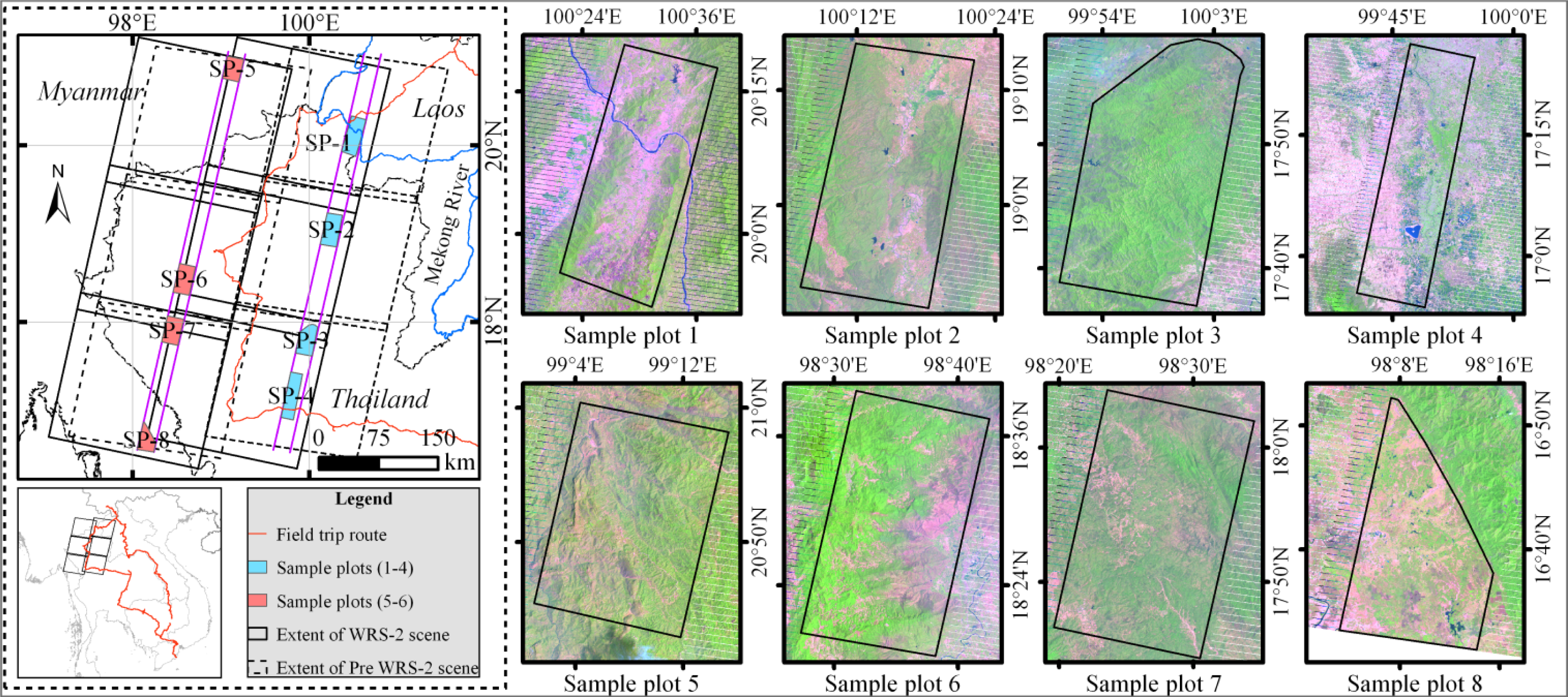
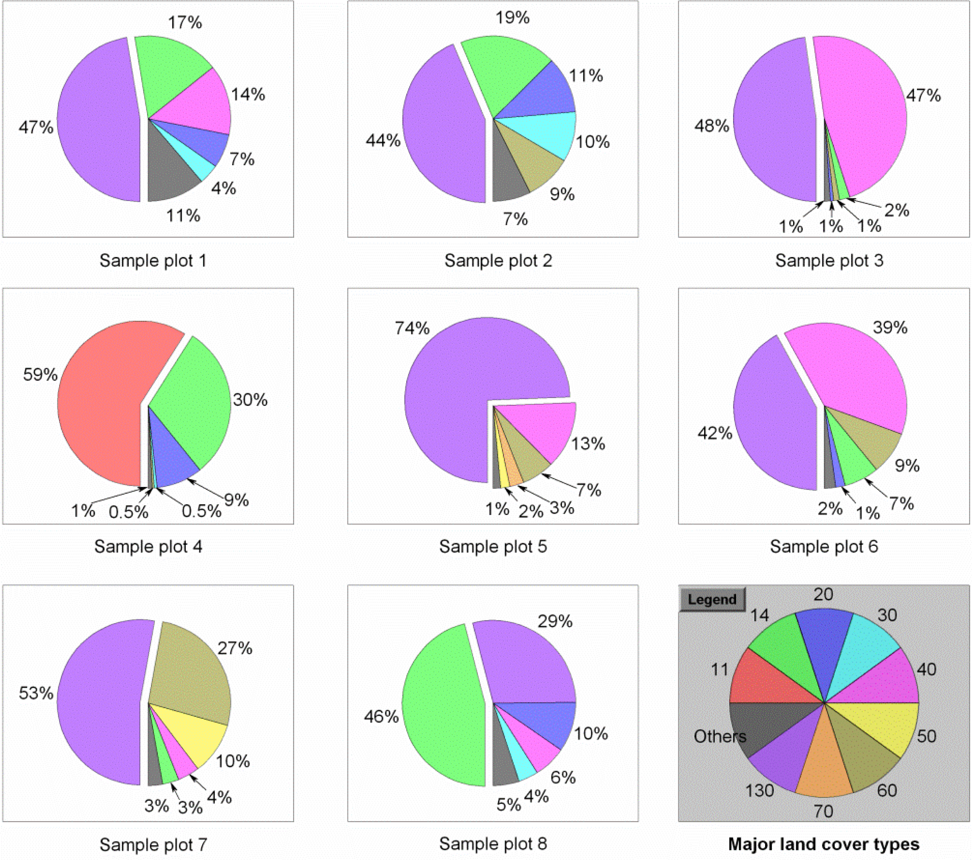
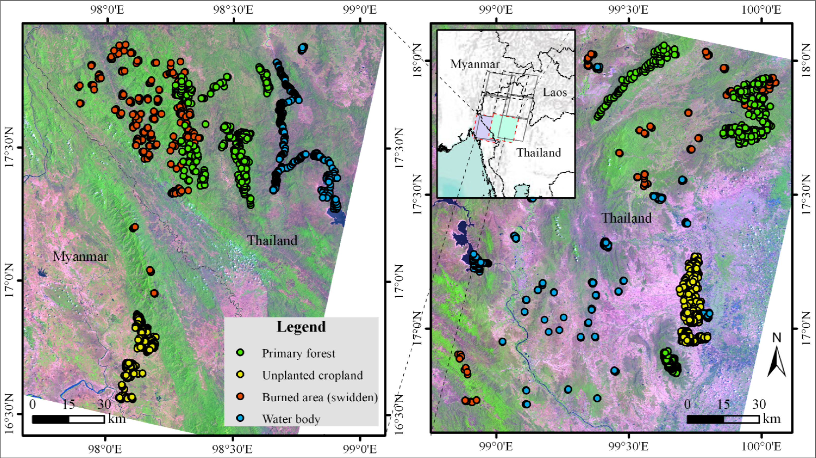
2.1. Ground Reference Data and Testing Sites

Field surveys of land use and land cover types were conducted in the Mekong River Basin, including Laos, Cambodia, Thailand and Vietnam, from 25 February 2013 to 17 March 2013. Using a Casio Exilim EX-H20G (with Hybrid GPS) camera and a Canon GP-E2 Camera GPS receiver, over 10,000 geo-referenced field photos along the field trip route in the four countries were gathered for selecting eight sample plots and sample points across the border area of Myanmar, Laos and Thailand. The thousands of photos were simultaneously taken in a bi-directional manner by a moving vehicle every 2–5 min. The field route traveled by the field team was collected with a handheld GPS receiver (Trimble Juno SB) in a counter-clockwise direction (Figure 2), from Laos, Cambodia to Vietnam and then back to Cambodia, Thailand and Laos. These field photos recorded specific information about land use and land cover types, such as primary or secondary forests, tree plantations (e.g., rubber, eucalyptus, teak, mangrove and fruit orchards), shrubland, grassland, swidden agriculture, croplands (e.g., paddy rice and cassava), village and towns, and so on.
The testing sites chosen for cross-comparison studies between ETM+ and OLI sensors are very important. Three basic rules for selecting sample plots were followed in this study: first, the time difference between both sensors observing the same place should be as short as possible. Usually, the side-by-side overlap between adjacent paths of Landsat-7 and Landsat-8 enables the area to be covered just one day apart. However, the gaps of ETM+ SLC-off images are noticeable along the edge of each scene and gradually reduce towards the scene center. For this reason, it is not appropriate to use the overlapping part of two scenes between adjacent paths. Second, the vegetation target types of sample plots should not encompass pronounced phenological features. For example, deciduous rubber trees start new leaf emergence, and many primary or secondary forests are slashed and burned for swidden cultivation in late March and April. This creates a rapid change in vegetation indices and is not suitable. Third, all the sample plots should be cloud free. Therefore, the border area of Myanmar, Laos and Thailand in Mainland Southeast Asia was chosen as the study area (Figure 2), because both sensors acquired cloud-free images during the period when Landsat-8 achieved operational orbit. Both sensors almost provide near-coincident data during this period.
This region has a tropical monsoon climate. There are three distinct seasons in Mainland Southeast Asia, i.e., the hot season from March to April, the cool and dry season from November to February and the rainy season from May to October [22]. During the dry season, natural landscape types are diverse and the differences among various landscapes are very evident. Land cover types include nine broad categories, such as primary forest, secondary forest (e.g., rubber/teak/eucalyptus plantations), shrubland, grassland, croplands, swidden cultivation (or slashed and burned plots), bare-land, built-up land and water bodies [23,24]. It is worthwhile to mention that swidden cultivation is a dominant land use type in Southeast Asia [25,26]. Swidden cultivation employs a natural or improved fallow phase, which is longer that the cultivation phase of annual crops, sufficiently long to be dominated by woody vegetation, and cleared by means of fire [27]. Additionally, there is infrequent or light cloudy weather during the hot and cool and dry seasons. The weather makes the acquisitions of cloud-free imagery possible for comparative analysis. For example, statistics from the USGS GloVis showed that there are 28 ETM+ or OLI scenes (Worldwide Reference System (WRS)-2 path/row = 130/046) with cloud coverage less than or equal to 10% during 2009–2013. Among them, 25 scenes were acquired from November to April, while only 3 scenes were available between May and October.
In this study, eight sample plots (polygons) covering diverse land cover types were manually selected within six pairs of scenes, which are only two days apart (Figure 2, Table 2). These polygons were longitudinally located and spanned over 500 km from north to south and about 150 km from west to east. Sample plot 1 is located in the border region of Laos and Thailand. Sample plot 2, 3, 4, 6 and 7 were all located in Northern Thailand, and sample plot 5 and 8 were located in Myanmar. Similarly, the selection of sampling areas abided by three rules: cloud free, located in the overlapping regions between the center part of the ETM+ SLC image and OLI image and diverse land cover types. According to the Global Land Cover Map 2009 products (also called GlobCover 2009) provided by the European Space Agency (ESA), five major land cover types of all sample plots were statistically evaluated (Figure 3). This shows that all the sample plots were normally closed to open shrubland, unplanted croplands and mosaic croplands/vegetation. Considering the coarse pixel resolution (300 m) of GlobCover 2009, these sample plots actually encompassed even more diverse land cover types. These sampling areas represent the highly different land cover types.
In addition, 1,528 independent random sample points of four major land cover types, i.e., primary forest (378), unplanted cropland (454), burned plots (342) and water body (354), were randomly selected within one pair of scenes (WRS-2 path/row = 131/048, 25 and 27 March 2013, Figure 4, left panel) in ArcGIS 10.0. Similarly, another 1,783 independent random sample points of primary forest (568), unplanted cropland (544), burned plots (255) and water body (416) were randomly selected within one pair of scenes (WRS-2 path/row = 131/048, 1 and 3 April 2013, Figure 4, right panel). The sample points of these land cover types were used to compare each spectral band of ETM+ and OLI. All these sample points were not affected by the SLC failure and cloud.

2.2. Landsat-7/8 Imagery and Pre-Processing

In order to enable cross-comparative analysis between Landsat-7 ETM+ and Landsat-8 OLI sensors, six pairs of scenes (12 in total) of the Landsat-7 ETM+ SLC-off data and Landsat-8 OLI/TIRS Pre Worldwide Reference System (WRS) 2 data (Table 3) were gathered. Landsat-7 ETM+ SLC-off data refers to the products that have data gaps collected after May 2003 [19]. Landsat-8 OLI/TIRS Pre-WRS-2 data refers to the products acquired before 10 April 2013 [21]. All these data meet the quality standards of the same radiometric and geometric correction, but the geographic extents of each scene differ [19,21]. However, there is an overlap part of over 60 percent of a scene between adjacent paths of two sensors. This overlap area can be covered by scenes from each sensor, which are only two days apart. Considering the SLC failure problem of Landsat-7 ETM+, this research only compares the overlapping areas between the middle of ETM+ scene and OLI images. All twelve Landsat images were available from the Global Visualization Viewer (GloVis, http://glovis.usgs.gov/) developed by the Earth Resource Observation and Science Center (EROS) of the USGS. They are standard level-one terrain-corrected (L1T) products, which have had systematic radiometric and geometric corrections and ensured the overall geometric accuracy with ground control points and a digital elevation model [28].
As earlier studies show, surface reflectance data serves as the prerequisite for comparative analysis of vegetation indices derived from different sensor systems [2]. In this study, each Landsat image has undergone atmospheric correction to convert digital number values into surface reflectance for vegetation indices calculation in the software of Environment for Visualizing Images (ENVI, Version 5.0 SP3, Exelis Visual Information Solutions, Boulder, CO, USA). ENVI has an atmospheric correction module for retrieving spectral reflectance, i.e., the Fast Line-of-sight Atmospheric Analysis of Spectral Hypercubes (FLAASH) [29]. FLAASH incorporates the Moderate Resolution Transmission (MODTRAN) 4 radiative transfer code [29]. Model parameters describing the tropical atmosphere and rural aerosols together with 2-band (K-T) aerosol retrieval were utilized in ENVI FLAASH.
Although the sample areas were comprised of multiple land cover types (Table 2) in the tropical humid region, they could be divided into three groups: natural vegetation, exposed soil (i.e., unplanted cropland and swidden field) and water body. The specific target types can be detected by spectral bands. For instance, the green band works for the identification of water bodies when combined with NIR or short-wave infrared (SWIR) 1 to form the Normalized Difference Water Index (NDWI) [30] and MNDWI [31]. The red and NIR bands are particularly useful for vegetation monitoring [32]. The SWIR 1/2 bands are sensitive to the moisture content of vegetation and soil [33]. Landsat family sensors (since Landsat-5) have all these bands. Therefore, another three commonly used indices, the MNDWI [31], LSWI [34] and NBR [35], as well as NDVI [32] were introduced to compare the difference and correlation of both sensors. The corresponding formulas are given as follows:
LSWI = ( ρ NIR ρ SWIR 1 ) / ( ρ NIR + ρ SWIR 1 )
NBR = ( ρ NIR ρ SWIR 2 ) / ( ρ NIR + ρ SWIR 2 )
NDVI = ( ρ NIR ρ Red ) / ( ρ NIR + ρ Red )
MNDWI = ( ρ Green ρ SWIR 1 ) / ( ρ Green + ρ SWIR 1 )
where ρgreen, ρred, ρNIR, ρSWIR1 and ρSWIR2 refer to the surface reflectance values of Band 2, Band 3, Band 4, Band 5 and Band 7 in the Landsat-7 ETM+ sensor and Band 3, Band 4, Band 5, Band 6 and Band 7 in the Landsat-8 OLI sensor (Table 1), respectively. As opposed to LSWI and MNDWI, NDVI and NBR are more widely used for cross-comparison analysis. LSWI is similar to NBR, as they were both computed with NIR and SWIR bands. It is appropriate to use LSWI for such an analysis. In contrast, MNDWI is less reported and may lead to SBDE.

2.3. Statistical Analysis

Statistical analysis methods are widely used in cross-comparison between various satellite sensors [1,2,4,10,15]. Statistical analysis mainly consists of three parts in this study. To begin with, based on the 3,311 sample points, the difference of each band of both sensors was cross-compared. Then, as there are only two days apart for six pairs of images, our hypothesis is that the difference values of four vegetation indices for shrubland and unplanted croplands at the pixel level should be very close to zero. The average values and standard deviations of differenced vegetation indices for eight polygons to demonstrate the similarity or difference between Landsat-7 ETM+ and Landsat-8 OLI sensor were cross-compared. Finally, scatter plots of vegetation indices for cross-comparisons were applied to calculate the coefficients of determination (R2) based on linear correlation analysis. Meanwhile, mean values of the slope and Y-intercept generated from linear regression were used to define linear inter-calibration equations for NDVI, LSWI, MNDWI and NBR between ETM+ and OLI.

3. Results and Discussion

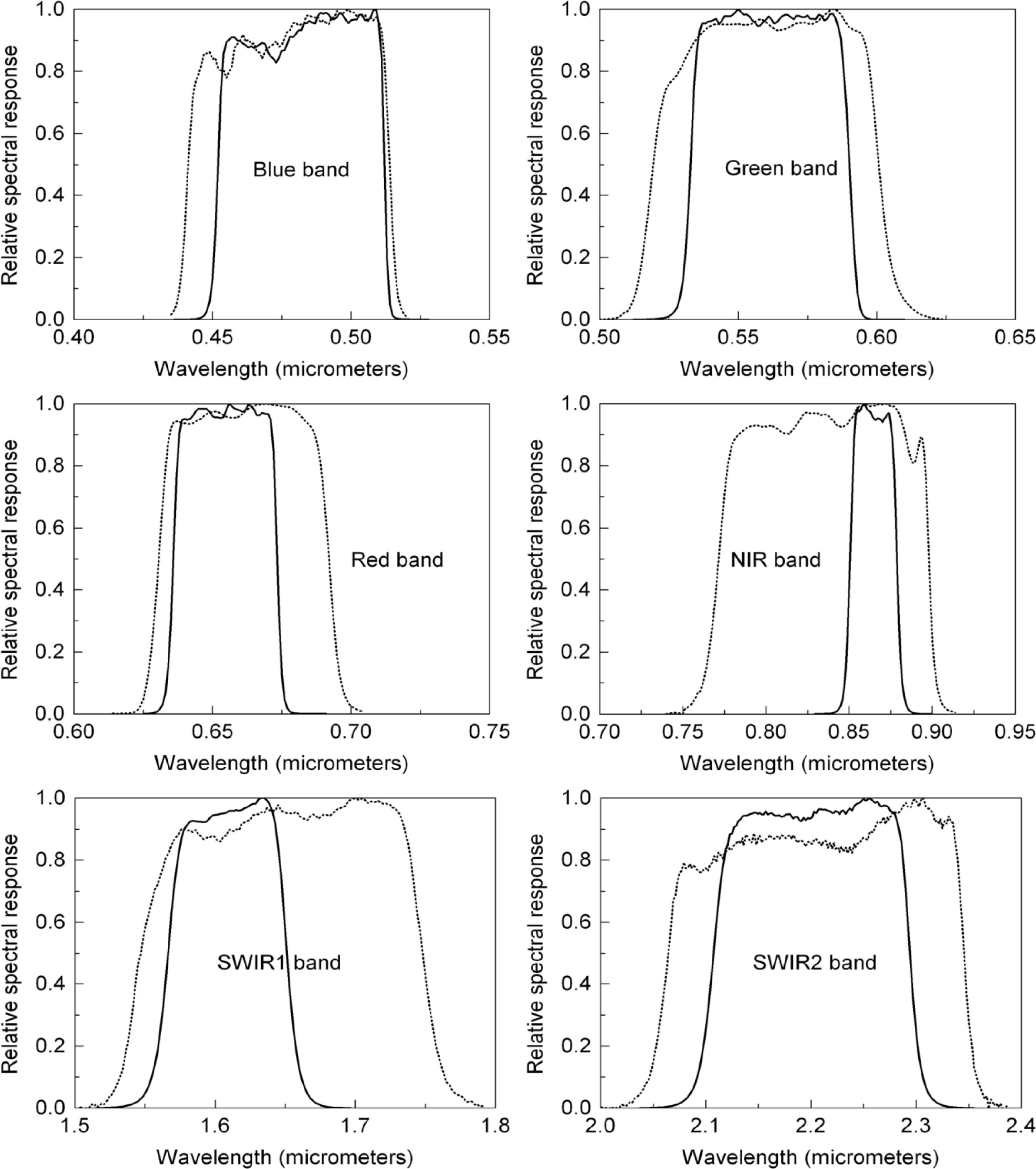
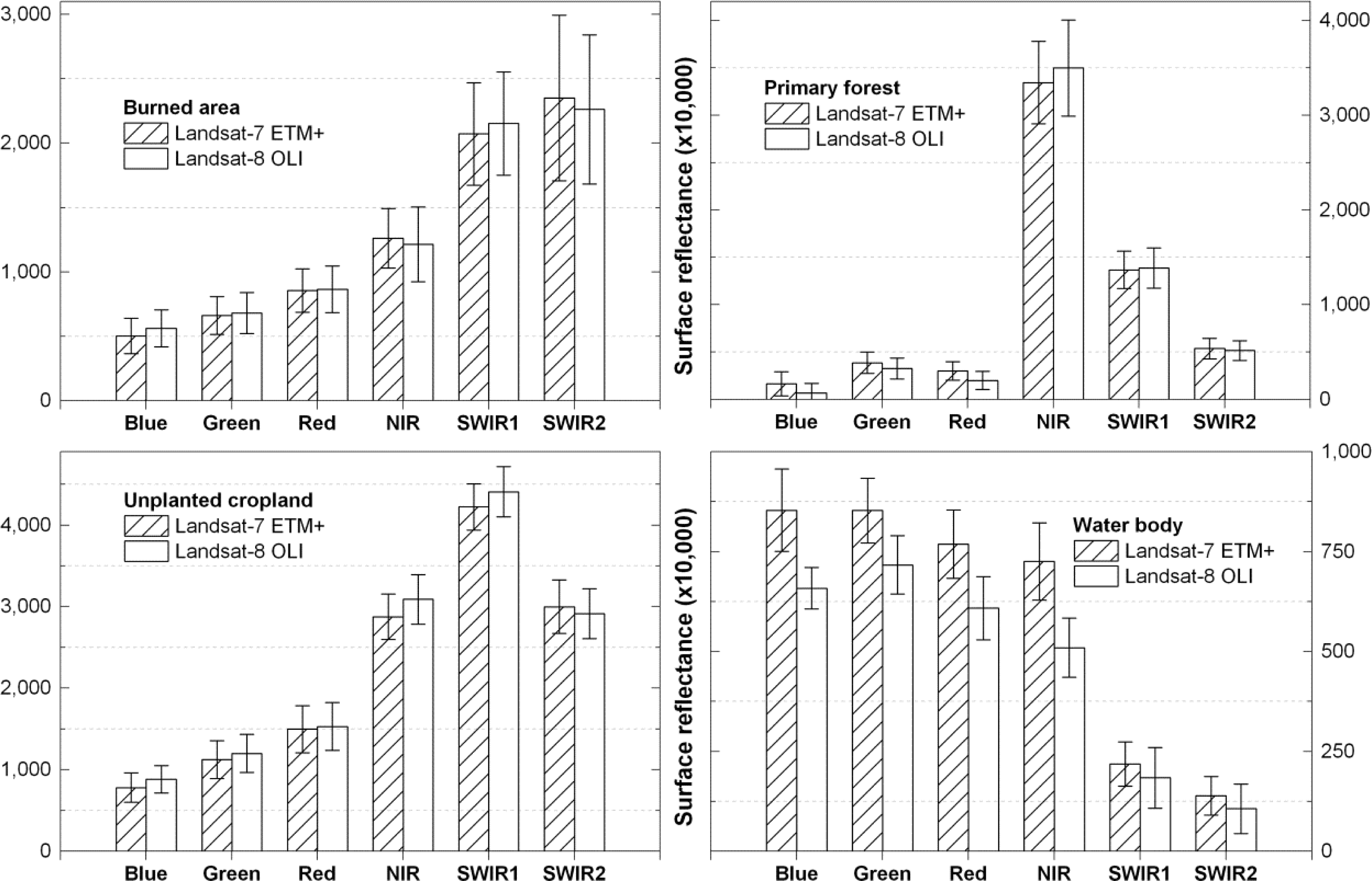
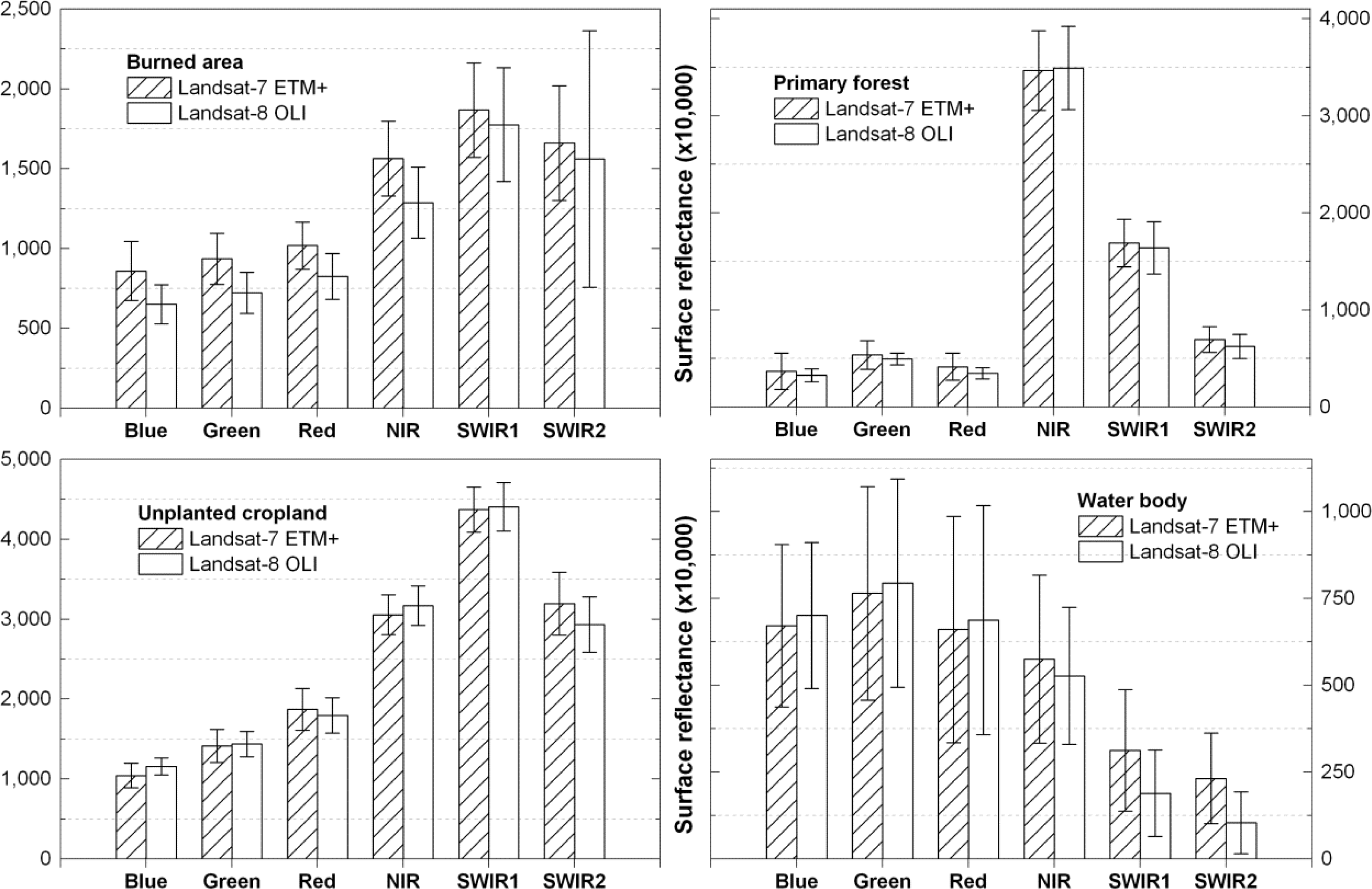
3.1. Comparison Landsat-7 ETM+ and Landsat-8 OLI Spectral Bands

Considering the chronological order difference of Landsat-7 and Landsat-8 imagery acquisition, two pairs of dates (or images) were utilized for band comparison, i.e., 25 March 2013(ETM+) and 27 March 2013 (OLI) and 1 April 2013(OLI) and 3 April 2013(ETM+). These time-interleaved Landsat scenes help to reduce the impacts of phenological features or weather fluctuation (e.g., showers) on comparative analysis between spectral bands. Then, surface reflectance values were extracted from each spectral band based on the 3,311 sample points of four land cover types. Figures 5 and 6, respectively, display the column plots of the surface reflectance of the spectral bands of both sensors extracted based on the 1,528 and 1,783 sample points. Comparative analysis between spectral bands of the ETM+ and OLI images acquired only two days apart showed that the average surface reflectance values of each band differed slightly. However, the relationship of the surface reflectance of related bands for different land cover types displayed high similarity between both sensors, as they are in analogous spectral regions. For example, the NIR band is very sensitive to growing vegetation (primary forest); SWIR bands are sensitive to soil-exposed land surface, e.g., burned area and unplanted cropland; and a combination of green and SWIR bands perform better in detecting water bodies.
Additionally, some important variations between ETM+ and OLI were obtained in this study. First, among the six spectral bands, only the average surface reflectance values of the SWIR 2 band of the OLI sensor for the four land cover types consistently decreased. Second, the average surface reflectance values of the NIR band of OLI for vegetative types (i.e., primary forest and unplanted cropland) increased slightly, while those for non-vegetative types (e.g., burned area and water body) decreased, on the contrary. It therefore could be concluded that the OLI sensor improved its performance in discriminating vegetative land cover from non-vegetative types. Third, the average surface reflectance values of the SWIR 1 band of OLI for non-water land cover types basically increased, while those for water bodies decreased. Fourth, the spectral bands of burned areas slightly increased over time, while the NIR and SWIR 2 bands further decreased. This highlights the potential for distinguishing burned areas from unburned areas with these bands. Fifth, the NIR and SWIR bands of the OLI sensor for water bodies decreased in comparison with those of the ETM+ sensor, while the visible bands showed completely inverse variations.

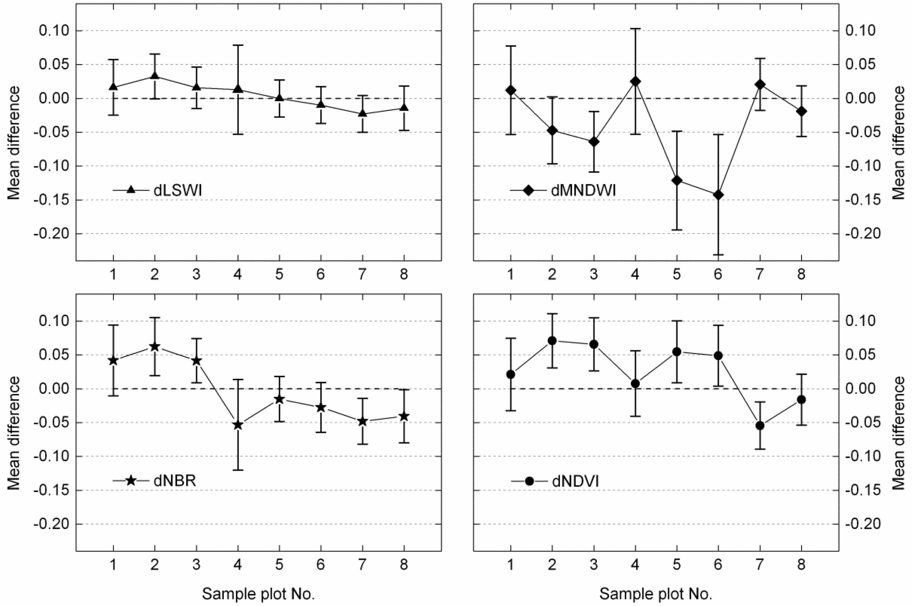
3.2. Comparison between the Values of Vegetation Indices Derived from ETM+ and OLI Sensors

Vegetation index values of eight sample plots derived from Landsat-8 OLI images acquired on 27 March 2013 and 1 April 2013 were used to compare with those derived from Landsat-7 ETM+ images acquired on 25 March 2013 and 3 April 2013. Pair comparative analysis of four vegetation indices (NDVI, LSWI, MNDWI and NBR) for each sample plot basically demonstrated that there existed subtle differences between the Landsat-7 ETM+ and Landsat-8 OLI sensors (Figure 7). This was clearly illustrated, especially by LSWI, NBR and NDVI, because their average difference values were less than ±0.05, and they had a smaller standard deviation. LSWI might be the optimum parameter (approximated to zero), which demonstrated a very high similarity of both sensors, followed by NBR and NDVI. However, MNDWI performed relatively poorly, because the average difference values reached up to −0.15. As shown in Figure 7, it was very important to note that vegetation indices calculated with non-visible spectral bands, mainly LSWI and NBR, were more stable for comparative analysis between the ETM+ and OLI sensors. The fluctuations of mean values of differenced vegetation indices (LSWI and NBR) among the eight sample plots were very small, less than 0.05. However, the average values of NDVI and MNDWI, calculated with visible and near-infrared or short-wave near-infrared spectral bands, either fluctuated obviously or were non-zero. Our analysis results also validated the possible spectral band difference effects (SBDEs) when using visible spectral bands for calculating vegetation indices [1,3]. Particularly, the SBDEs caused by the red band were far less than the green band. This is evidenced by the large standard deviation of difference values of MNDWI. It therefore could be concluded that the notable fluctuation of difference values of MNDWI among sample plots might be induced by the SBDE.
Another factor that led to the fluctuation of the difference values of vegetation indices might be the different land cover types among eight sample plots. As displayed in Figure 7, the difference values of vegetation indices for unplanted croplands dominated the landscape (i.e., sample plot 1, 4 and 8) and were basically less than ±0.02. However, the difference values of NBR (nearly ±0.05) were greater than those of the other three indices on the whole. This anomaly might have a close connection with cropland burning during the hot season [36,37]. Actually, we indeed noticed that the vast area of croplands were uncultivated because of a shortage of irrigation water during our field trip in northern Thailand. The weeds and crop residuals in the croplands turned yellow. Some fields had been burned, while other more were waiting for burning in the next few days.

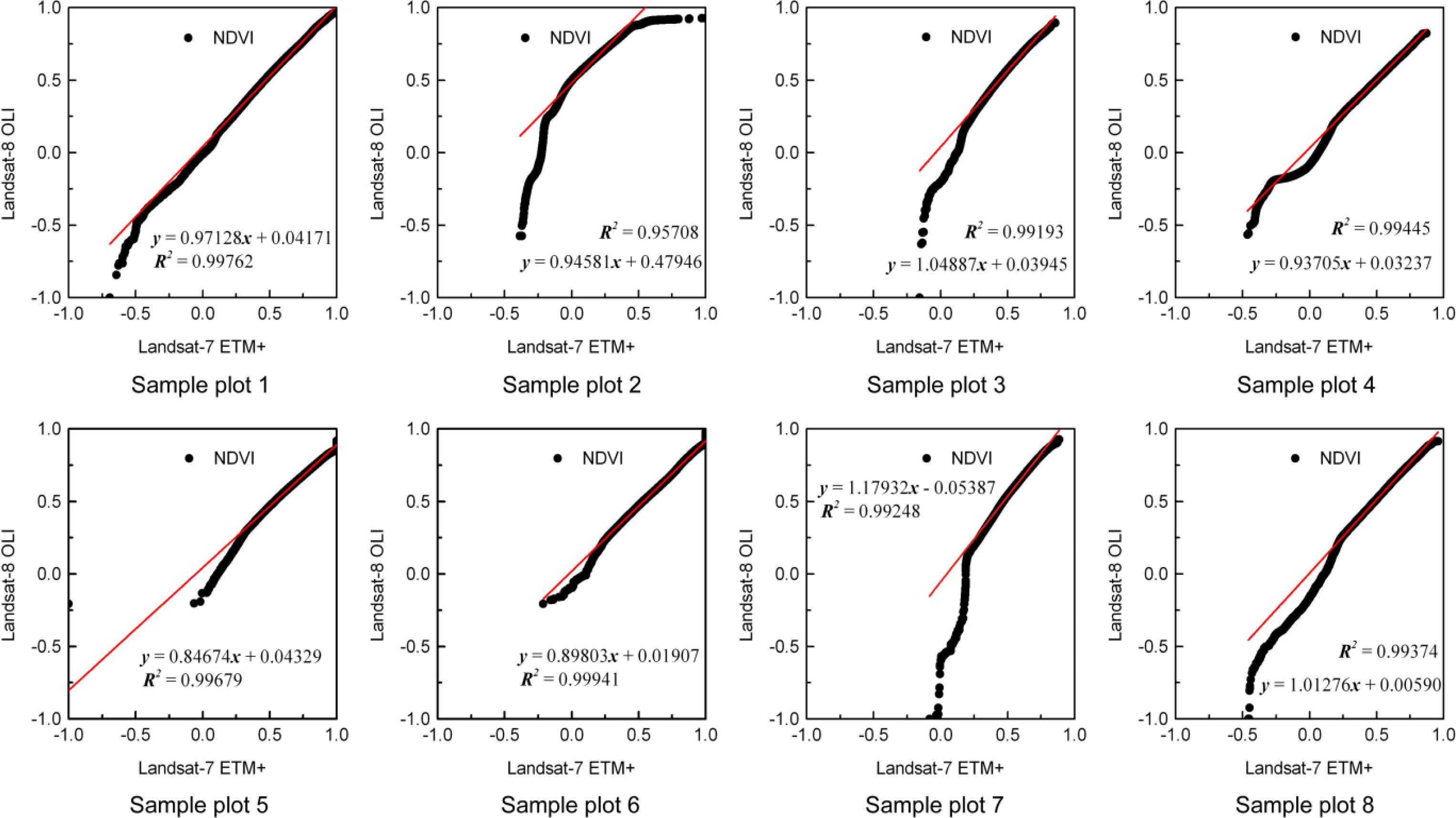
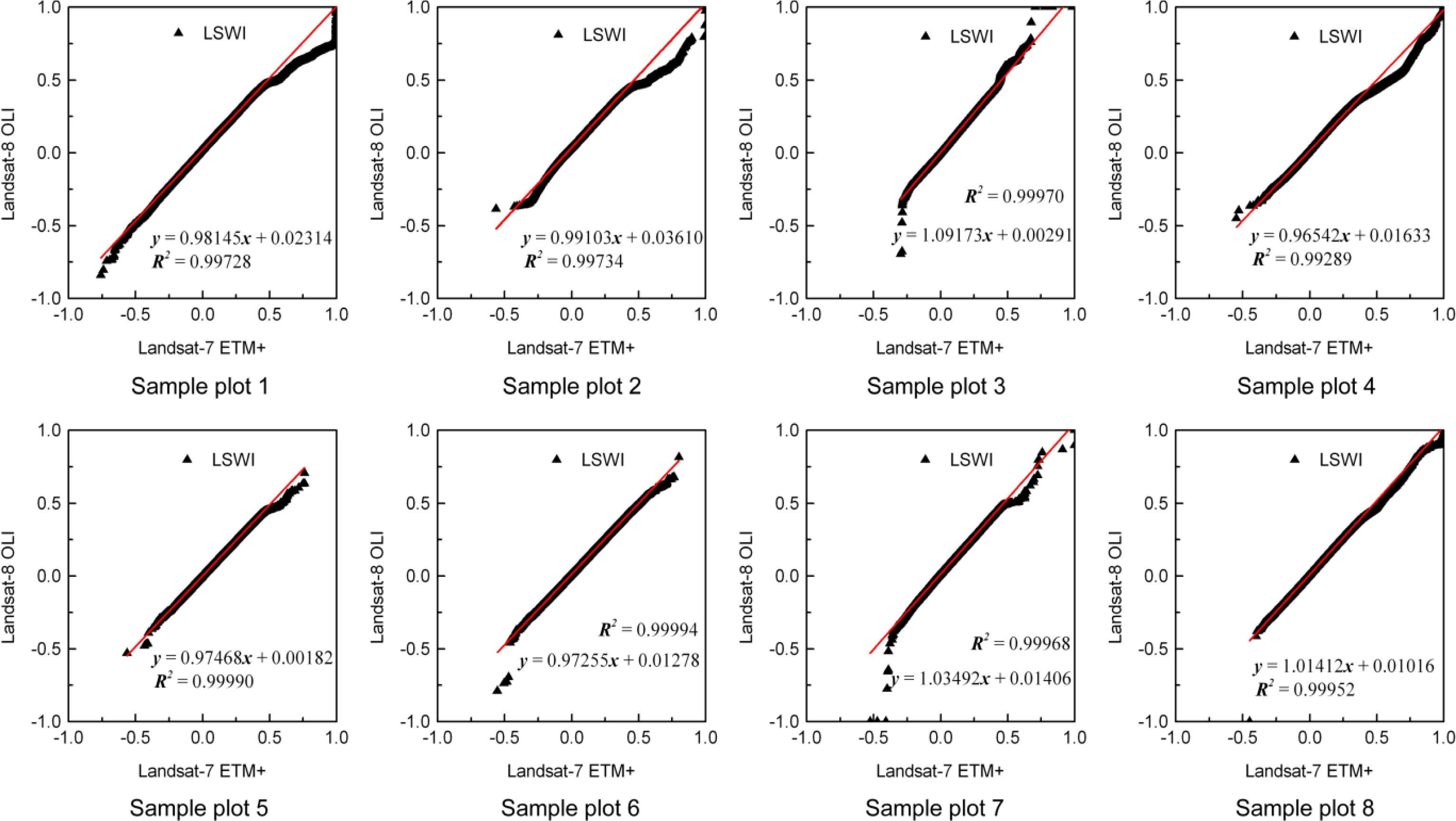
3.3. Correlation Analysis of Vegetation Indices Derived from ETM+ and OLI

Scatter plots with correlation coefficients of vegetation indices (NDVI, LSWI, MNDWI and NBR) consistently showed that the imagery acquired two days apart has very high correlation between Landsat-7 ETM+ and Landsat-8 OLI (Figures 8 and 11). In each plot, Landsat-8 OLI-derived vegetation indices are displayed on the Y-axis, while Landsat-7 ETM+-derived vegetation indices are shown on the X-axis. Coefficients of determination (R2) of each plot were greater than 0.96 on the whole. They demonstrated that vegetation indices obtained from Landsat-7 ETM+ and Landsat-8 OLI were highly linearly correlated. Therefore, it can be concluded that the imagery of both sensors can be used as complementary data. For all eight sample plots, the mean values of slope and the Y-intercept were used to form the inter-calibration equations of vegetation indices between Landsat-7 ETM+ and Landsat-8 OLI imagery as follows:
Intercalibrated   LSWI Landsat 8 OLI = 1.00324 * LSWI Landsat 7 ETM + + 0.01466
Intercalibrated   NBR Landsat 8 OLI = 0.95342 * NBR Landsat 7 ETM + + 0.05844
Intercalibrated   NDVI Landsat 8 OLI = 0.97998 * NDVI Landsat 7 ETM + + 0.07592
Intercalibrated   MNDWI Landsat 8 OLI = 0.88513 * MNDWI Landsat 7 ETM + 0.04079
However, there still existed some differences among the four vegetation indices. To begin with, the two indices (LSWI and NBR), computed from the near-infrared (NIR) and short-wave infrared (SWIR 1/2) bands, had slightly larger R2 values (over 0.99) than those of NDVI and MNDWI, which are computed using visible bands (the red and green bands) and the NIR/SWIR bands for each sample plot. The NBR obtained the highest average R2 value (0.999), while the MNDWI got the lowest (0.983) among eight sample plots. Then, the LSWI and NBR were highly correlated and basically followed the 1:1 line, while the NDVI and MNDWI also had high correlation coefficients, but did not always follow the 1:1 line. The fluctuations of NDVI and MNDWI values extracted from both sensors further proved the potential spectral band difference effects (SBDEs). Based on Equations (58), the slope values are close to 1.0 when converting vegetation indices values of Landsat-7 ETM+ into those of Landsat-8 OLI, but only NDVI and MNDWI values deviated from the fitted curve in each plot of Figures 8 and 10. There were differences for the lower values of NDVI and higher values of MNDWI.

4. Conclusions

Landsat-8 restarted the multi-decadal Landsat data record of global surface changes after Landsat-5 discontinued its Earth observation, and Landsat-7 has continuous problems in SLC and limited fuel [3,4,38]. Currently, Landsat-8 and Landast-7 will assure an eight-day repeat coverage for monitoring the entire Earth, especially for mapping crop growth and forest disturbances. Consequently, comparison analysis between Landsat-8 and its predecessors will be of significant importance for detecting spatial and temporal land surface changes, since the Landsat satellites have collected invaluable global imagery for over 40 years [39].
In this study, practical and repeatable comparative analyses of Landsat-7 ETM+ and Landsat-8 OLI were carried out from two aspects: spectral bands comparison with sample points and vegetation indices comparison with sample plots. We used Landsat imagery (ETM+ SLC-off and OLI Pre-WRS-2 data) that was just two days apart, which helps to reduce the impacts of phenology and weather fluctuations. Spectral bands comparison of both sensors showed that the spectral bands differed slightly, but with high similarities. Specifically, in comparing with ETM+, first, the OLI had higher values of the near-infrared band for vegetative land cover types, but lower values for non-vegetative types. Second, the new sensor had lower values for the shortwave infrared (2.11–2.29 μm) band for all land cover types. Third, it also basically had higher values for the shortwave infrared (1.57–1.65 μm) band for non-water land cover types. The difference of vegetation indices comparison showed that there were subtle differences between both sensors, which demonstrated high similarity. LSWI, NBR and NDVI had average difference values less than ±0.05 and a smaller standard deviation. LSWI might be the optimum parameter (approximated to zero), followed by NBR and NDVI. However, MNDWI performed relatively poorly, because the average difference values reached up to −0.15. Additionally, correlation analysis of the vegetation indices indicated that both sensors had a very high linear correlation coefficient, with R2 greater than 0.96. The subtle differences and high correlation of vegetation indices demonstrated that ETM+ and OLI imagery can be used as complementary data. Lastly, the NIR and SWIR bands-calculated vegetation indices (i.e., LSWI and NBR) performed better than NDVI and MNDWI for cross-comparison analysis of satellite sensors, due to the spectral band difference effects.
To our knowledge, this study may be the first comparative analysis between Landsat-8 OLI and Landsat-7 ETM+. It preliminarily compares the difference and correlation of spectral bands and vegetation indices from both sensors. However, it is worthwhile to emphasize that more comparison analysis between Landsat-8 OLI/TIRS and other sensors should be carried out in the future. As the band wavelength gets shorter and the entire detector system changes from whisk-broom to push-broom design [18], related comparative studies between Landsat-8 OLI/TIRS and previous Landsat satellites will deserve more attention. Such research work will lay the foundation for integrating historical Landsat imagery over 40 years for monitoring the spatio-temporal change, pattern and process of the Earth ecosystem.

Acknowledgments

This research was supported by the National Natural Science Foundation of China (No. 41301090 and 41271117) and the Key Program for Strategic Science and Technology, the Chinese Academy of Sciences (No. 2012SJ008). Landsat-7/8 imagery is available from the US Geological Survey (USGS) EROS Data Center. We thank five anonymous reviewers for their thoughtful and constructive suggestion and comments on earlier versions of this manuscript.

Conflicts of Interest

The authors declare no conflict of interest.

References

  1. Anderson, J.H.; Weber, K.T.; Gokhale, B.; Chen, F. Intercalibration and evaluation of Resourcesat-1 and Landsat-5 NDVI. Can. J. Remote Sens 2011, 37, 213–219. [Google Scholar]
  2. Steven, M.D.; Malthus, T.J.; Baret, F.; Xu, H.; Chopping, M.J. Intercalibration of vegetation indices from different sensor systems. Remote Sens. Environ 2003, 88, 412–422. [Google Scholar]
  3. Teillet, P.M.; Ren, X. Spectral band difference effects on vegetation indices derived from multiple satellite sensor data. Can. J. Remote Sens 2008, 34, 159–173. [Google Scholar]
  4. Chen, X.; Vogelmann, J.E.; Chander, G.; Ji, L.; Tolk, B.; Huang, C.; Rollins, M. Cross-sensor comparisons between Landsat 5 TM and IRS-P6 AWiFS and disturbance detection using integrated Landsat and AWiFS time-series images. Int. J. Remote Sens 2013, 34, 2432–2453. [Google Scholar]
  5. Teillet, P.M.; Fedosejevs, G.; Thome, K.J.; Barker, J.L. Impacts of spectral band difference effects on radiometric cross-calibration between satellite sensors in the solar-reflective spectral domain. Remote Sens. Environ 2007, 110, 393–409. [Google Scholar]
  6. Dinguirard, M.; Slater, P.N. Calibration of space-multispectral imaging sensors: A review. Remote Sens. Environ 1999, 68, 194–205. [Google Scholar]
  7. Oguro, Y.; Tsuchiya, K.; Suga, Y. Comparison of land cover features observed with different satellite sensors over a semi-arid land in central Australia. Adv. Space Res 1999, 23, 1401–1404. [Google Scholar]
  8. Oguro, Y.; Suga, Y.; Takeuchi, S.; Ogawa, M.; Konishi, T.; Tsuchiya, K. Comparison of SAR and optical sensor data for monitoring of rice plant around Hiroshima. Adv. Space Res 2001, 28, 195–200. [Google Scholar]
  9. Oguro, Y.; Suga, Y.; Takeuchi, S.; Ogawa, H.; Tsuchiya, K. Monitoring of a rice field using Landsat-5 TM and Landsat-7 ETM+ data. Adv. Space Res 2003, 32, 2223–2228. [Google Scholar]
  10. Van Wagtendonk, J.W.; Root, R.R.; Key, C.H. Comparison of AVIRIS and Landsat ETM+ detection capabilities for burn severity. Remote Sens. Environ 2004, 92, 397–408. [Google Scholar]
  11. Vazquez, A.; Cuevas, J.M.; Gonzalez-Alonso, F. Comparison of the use of WiFS and LISS images to estimate the area burned in a large forest fire. Int. J. Remote Sens 2001, 22, 901–907. [Google Scholar]
  12. Hill, J.; Aifadopoulou, D. Comparative analysis of Landsat-5 TM and SPOT HRV-1 data for use in multiple sensor approaches. Remote Sens. Environ 1990, 34, 55–70. [Google Scholar]
  13. Tsuchiya, K.; Oguro, Y. Comparison of remotely sensed data obtained with various sensors over an arid zone. Adv. Space Res 1997, 19, 1383–1386. [Google Scholar]
  14. Suga, Y.; Oguro, Y.; Takeuchi, S.; Tsuchiya, K. Comparison of various SAR data for vegetation analysis over Hiroshima City. Adv. Space Res 1999, 23, 1509–1516. [Google Scholar]
  15. Teillet, P.M.; Barker, J.L.; Markham, B.L.; Irish, R.R.; Fedosejevs, G.; Storey, J.C. Radiometric cross-calibration of the Landsat-7 ETM+ and Landsat-5 TM sensors based on tandem data sets. Remote Sens. Environ 2001, 78, 39–54. [Google Scholar]
  16. Serra, P.; Pons, X.; Sauri, D. Post-classification change detection with data from different sensors: Some accuracy considerations. Int. J. Remote Sens 2003, 24, 3311–3340. [Google Scholar]
  17. Holden, Z.A.; Morgan, P.; Smith, A.; Vierling, L. Beyond Landsat: A comparison of four satellite sensors for detecting burn severity in ponderosa pine forests of the Gila Wilderness, NM, USA. Int. J. Wildland Fire 2010, 19, 449–458. [Google Scholar]
  18. Irons, J.R.; Dwyer, J.L.; Barsi, J.A. The next Landsat satellite: The Landsat data continuity mission. Remote Sens. Environ 2012, 122, 11–21. [Google Scholar]
  19. USGS. What is Landsat 7 ETM+ SLC-off data? http://landsat.usgs.gov/Landsat_7_ETM_SLC_off_data.php (accessed on 8 November 2013).
  20. Markham, B.L.; Knight, E.J.; Canova, B.; Donley, E.; Kvaran, G.; Lee, K.; Barsi, J.A.; Pedelty, J.A.; Dabney, P.W.; Irons, J.R. The Landsat Data Continuity Mission Operational Land Imager (OLI) Sensor. Proceedings of 2012 IEEE International Geoscience and Remote Sensing Symposium (IGARSS), Munich, Germany, 1 January 2012; pp. 6995–6998.
  21. USGS. What is Landsat 8 OLI/TIRS Pre-WRS-2 data? Available online: http://landsat.usgs.gov/L8_Pre_WRS2.php (accessed on 8 November 2013).
  22. Taylor, D. Biomass burning, humans and climate change in Southeast Asia. Biodivers. Conserv 2010, 19, 1025–1042. [Google Scholar]
  23. Fox, J.; Vogler, J.B.; Sen, O.L.; Giambelluca, T.W.; Ziegler, A.D. Simulating land-cover change in montane mainland southeast Asia. Environ. Manag 2012, 49, 968–979. [Google Scholar]
  24. Fox, J.; Vogler, J.B. Land-use and land-cover change in montane mainland southeast Asia. Environ. Manag 2005, 36, 394–403. [Google Scholar]
  25. Padoch, C.; Coffey, K.; Mertz, O.; Leisz, S.J.; Fox, J.; Wadley, R.L. The demise of swidden in Southeast Asia? Local realities and regional ambiguities. Geogr. Tidsskr 2007, 107, 29–41. [Google Scholar]
  26. Schmidt-Vogt, D.; Leisz, S.J.; Mertz, O.; Heinimann, A.; Thiha, T.; Messerli, P.; Epprecht, M.; Cu, P.V.; Chi, V.K.; Hardiono, M.; et al. An assessment of trends in the extent of Swidden in southeast Asia. Human Ecol 2009, 37, 269–280. [Google Scholar]
  27. Mertz, O.; Padoch, C.; Fox, J.; Cramb, R.; Leisz, S.; Lam, N.; Vien, T. Swidden change in southeast Asia: Understanding causes and consequences. Human Ecol 2009, 37, 259–264. [Google Scholar]
  28. NASA Goddard Space Flight Center. Landsat 7 Science Data Users Handbook. Available online: http://landsathandbook.gsfc.nasa.gov/pdfs/Landsat7_Handbook.pdf (accessed on 8 November 2013).
  29. Exelis. ENVI Atmospheric Correction Module: QUAC and FLAASH User’s Guide. Available online: http://www.exelisvis.com/portals/0/pdfs/envi/Flaash_Module.pdf (accessed on 8 November 2013).
  30. McFeeters, S.K. The use of the Normalized Difference Water Index (NDWI) in the delineation of open water features. Int. J. Remote Sens 1996, 17, 1425–1432. [Google Scholar]
  31. Xu, H. Modification of normalised difference water index (NDWI) to enhance open water features in remotely sensed imagery. Int. J. Remote Sens 2006, 27, 3025–3033. [Google Scholar]
  32. Tucker, C.J. Red and photographic infrared linear combinations for monitoring vegetation. Remote Sens. Environ 1979, 8, 127–150. [Google Scholar]
  33. Tucker, C.J. Remote sensing of leaf water content in the near infrared. Remote Sens. Environ 1980, 10, 23–32. [Google Scholar]
  34. Xiao, X.M.; Zhang, Q.Y.; Saleska, S.; Hutyra, L.; de Camargo, P.; Wofsy, S.; Frolking, S.; Boles, S.; Keller, M.; Moore, B. Satellite-based modeling of gross primary production in a seasonally moist tropical evergreen forest. Remote Sens. Environ 2005, 94, 105–122. [Google Scholar]
  35. García, M.L.; Caselles, V. Mapping burns and natural reforestation using Thematic Mapper data. Geocarto Int 1991, 6, 31–37. [Google Scholar]
  36. Lin, H.; Jin, Y.; Giglio, L.; Foley, J.A.; Randerson, J.T. Evaluating greenhouse gas emissions inventories for agricultural burning using satellite observations of active fires. Ecol. Appl 2012, 22, 1345–1364. [Google Scholar]
  37. Giglio, L.; Csiszar, I.; Justice, C.O. Global distribution and seasonality of active fires as observed with the Terra and Aqua Moderate Resolution Imaging Spectroradiometer (MODIS) sensors. J. Geophys. Res.: Biogeosci 2006, 111. [Google Scholar] [CrossRef]
  38. Tollefson, J. Landsat 8 to the rescue. Nature 2013, 494, 13–14. [Google Scholar]
  39. Lulla, K.; Nellis, M.D.; Rundquist, B. Celebrating 40 years of Landsat program’s Earth observation accomplishments. Geocarto Int 2012, 27, 459. [Google Scholar]
Figure 1. Relative spectral response (RSR) profiles showing the spectral band difference between Landsat-8 Operational Land Imager (OLI) (solid curve) and Landsat-7 Enhanced Thematic Mapper Plus (ETM+) (short dot curve). Note that these response metadata are available from the web page of the Spectral Characteristics Viewer ( http://landsat.usgs.gov/tools_spectralViewer.php) provided by the US Geological Survey (USGS). SWIR, short-wave infrared.
Remotesensing 06 00310f1
Figure 2. Locations of the eight sample plots in Mainland Southeast Asia showing the corresponding land cover types imaged in the scenes of Landsat-7 ETM+ on 25 March 2013 and 3 April 2013. The two pairs of purple solid lines refer to the central part of ETM+ Scan Line Corrector (SLC)-off scenes with the eight sample plots included. WRS, Worldwide Reference System.
Remotesensing 06 00310f2
Figure 3. Area proportions of five major land use and land cover types within the eight sample plots in this study. The land cover data was extracted from the GlobCover 2009 provided by the European Space Agency (ESA). The figures in the legend plot refer to the land cover type codes of the global land cover dataset.
Remotesensing 06 00310f3
Figure 4. Locations of the 3,311 independent random sample points of four major land cover types in the border area of Myanmar and Thailand. The displayed images are Landsat-8 Pre-WRS-2 products acquired on 27 March 2013 (left) and 1 April 2013 (right).
Remotesensing 06 00310f4
Figure 5. Band differences of Landsat-7 ETM+ and Landsat-8 OLI images (25 March 2013 and 27 March 2013) for four land-cover types (primary forest, unplanted cropland, swidden field and water body).
Remotesensing 06 00310f5
Figure 6. Band differences of Landsat-7 ETM+ and Landsat-8 OLI images (3 April 2013 and 1 April 2013) for four land-cover types (primary forest, unplanted cropland, swidden field and water body).
Remotesensing 06 00310f6
Figure 7. Mean values and standard deviation of differenced vegetation indices (dLSWI, dMNDWI, dNBR and dNDVI) derived from Landsat-7 ETM+ images (25 March 2013 and 1 April 2013) and Landsat-8 OLI images (27 March 2013 and 3 April 2013) within eight sample plots. LSWI, Land Surface Water Index; MNDWI, Modified Normalized Difference Water Index (MNDWI); NBR, Normalized Burn Ratio; NDVI, Normalized Difference Vegetation Index.
Remotesensing 06 00310f7
Figure 8. Statistical relationship between Landsat-7 ETM+ and Landsat-8 OLI NDVI values for the eight sample plots. The linear regression equation and R2 value are given in each plot. The red solid line refers to the linear fitting curve.
Remotesensing 06 00310f8
Figure 9. Statistical relationship between Landsat-7 ETM+ and Landsat-8 OLI LSWI values for the eight sample plots. The linear regression equation and R2 value are given in each plot. The red solid line refers to the linear fitting curve.
Remotesensing 06 00310f9
Figure 10. Statistical relationship between Landsat-7 ETM+ and Landsat-8 OLI MNDWI values for the eight sample plots. The linear regression equation and R2 value are given in each plot. The red solid line refers to the linear fitting curve.
Remotesensing 06 00310f10
Figure 11. Statistical relationship between Landsat-7 ETM+ and Landsat-8 OLI NBR values for the eight sample plots. The linear regression equation and R2 value are given in each plot. The red solid line refers to the linear fitting curve.
Remotesensing 06 00310f11
Table 1. Comparison of Landsat-7 ETM+ and Landsat-8 OLI/Thermal Infrared Sensor (TIRS) spectral bands.
Landsat-8 OLI and TIRSLandsat-7 ETM+Resolution (m)

BandsWavelength (μm)BandsWavelength (μm)
Band 1—Coastal aerosol0.43–0.45NA--30
Band 2—Blue0.45–0.51Band 10.45–0.5230
Band 3—Green0.53–0.59Band 20.52–0.6030
Band 4—Red0.64–0.67Band 30.63–0.6930
Band 5—Near infrared (NIR)0.85–0.88Band 40.77–0.9030
Band 6—Short-wave infrared (SWIR 1)1.57–1.65Band 51.55–1.7530
Band 7—Short-wave infrared (SWIR 2)2.11–2.29Band 72.09–2.3530
Band 8—Panchromatic0.50–0.68Band 80.52–0.9015
Band 9—Cirrus1.36–1.38NA--30
Band 10—Thermal infrared (TIRS) 110.60–11.19Band 610.40–12.50TIRS/ETM+: 100/60 * (30)
Band 11—Thermal infrared (TIRS) 211.50–12.51
*ETM+ band 6 and TIRS thermal bands are acquired at the resolution of 60 and 100 meters, respectively, but all are resampled to 30-meter pixels in the delivered data product. The above information was compiled from the USGS Landsat Missions webpage ( http://landsat.usgs.gov/band_designations_landsat_satellites.php).
Table 2. Size and land cover structure of the selected sample plots.
Sample Plot No.Perimeter (km)Area (km2)Pixel NumberLand cover
Five Major Types*Cumulative Ratio
Sample plot 1129.55846.58940,648130 > 14 > 40 > 20 > 3089%
Sample plot 2118.07759.26843,627130 > 14 > 20 > 30 > 6093%
Sample plot 3109.19705.53783,927130 > 40 > 14 > 60 > 2099%
Sample plot 4146.16865.93962,15611 > 14 > 20 > 30 > 6099%
Sample plot 595.95555.01616,685130 > 40 > 60 > 70 > 5099%
Sample plot 6111.61705.52783,907130 > 40 > 60 > 14 > 2098%
Sample plot 7105.90654.93727,693130 > 60 > 50 > 40 > 1497%
Sample plot 897.00485.34539,26214 > 130 > 20 > 40 > 3095%
*Note that the values in bold refer to the land cover type codes extracted from the GlobCover 2009, respectively. 11: Post-flooding or irrigated croplands; 14: Rainfed croplands; 20: Mosaic cropland (50%–70%)/vegetation (grassland, shrubland, forest) (20%–50%); 30: Mosaic vegetation (grassland, shrubland, forest) (50%–70%)/cropland (20%–50%); 40: Closed to open (>15%) broadleaved evergreen and/or semi-deciduous forest (>5 m); 50: Closed (>40%) broadleaved deciduous forest (>5 m); 60: Open (15%–40%) broadleaved deciduous forest (>5 m); 70: Closed (>40%) needle-leaved evergreen forest (>5 m); 130: Closed to open (>15%) shrubland (<5 m).
Table 3. Landsat-7 ETM+ and Landsat-8 OLI images used in this study.
SensorAcquisition DatePath/RowCloud CoverageImagery Type
Landsat-7 ETM+25 March 2013131/046, 131/047 and 131/0482%, 0% and 1%Landsat-7 ETM+ SLC-off
3 April 2013130/046, 130/047 and 130/0480%, 1% and 0%Landsat-7 ETM+ SLC-off
Landsat-8 OLI27 March 2013131/046, 131/047 and 131/0480%, 0% and 2%Landsat-8 OLI/TIRS Pre-WRS-2
1 April 2013130/046, 130/047 and 130/0482%, 0% and 0%Landsat-8 OLI/TIRS Pre-WRS-2

