Homogeneity Analysis of the CM SAF Surface Solar Irradiance Dataset Derived from Geostationary Satellite Observations

Abstract

A satellite-based climate record of monthly mean surface solar irradiance (SIS) is investigated with regard to possible inhomogeneities in time. The data record is provided by the European Organisation for the Exploitation of Meteorological Satellites (EUMETSAT) Satellite Application Facility on Climate Monitoring (CM SAF) for the period of 1983 to 2005, covering a disk area between ±70° in latitude and longitude. The Standard Normal Homogeneity Test (SNHT) and two other homogeneity tests are applied with and without the use of reference SIS data (from the Baseline Surface Radiation Network (BSRN) and from the ECMWF (European Centre for Medium-Range Weather Forecasts) ERA -Interim reanalysis. The focus is on the detection of break-like inhomogeneities, which may occur due to satellite or SIS retrieval algorithm changes. In comparison with the few suitable BSRN SIS observation series with limited extension in time (no data before 1992), the CM SAF SIS time series do not show significant inhomogeneities, even though slight discrepancies in the surface measurements appear. The investigation of the full CM SAF SIS domain reveal inhomogeneities related to most of the documented satellite and retrieval changes, but only for relatively small domain fractions (especially in mountainous desert-like areas in Africa). In these regions the retrieval algorithm is not capable of adjusting for the changes of the satellite instruments. For other areas, e.g., Europe, no such breaks in the time series are found. We conclude that the CM SAF SIS data record has to be further assessed and regionally homogenized before climate trend investigations can be conducted.

1. Introduction

The solar radiation incident at the Earth’s surface, denoted in the following as SIS (surface incoming solar irradiance), is a major contributor to the surface energy budget and, thus, substantially determines the prevailing climatic conditions [1]. In addition, the amount of the incident surface solar radiation is highly relevant for the generation of electricity using solar energy technology. Thus, global high-quality observations of the incoming solar surface radiation are of major scientific and commercial interest.

Direct surface measurements of SIS are available for approximately 90 years, e.g., [2]. However, the number and quality of continuous time series covering time periods of several decades are limited. With the Baseline Surface Radiation Network (BSRN), established in 1992, highly accurate SIS measurements have become available at certain sites (currently more than 50). The BSRN data, intended for monitoring long-term changes of SIS and for the evaluation of satellite and climate model datasets [3], have been used in numerous studies dealing with the surface radiation budget [4] and the references therein. The surface observations available for SIS indicate a decrease until the 1980s (the so-called “global dimming”) followed by an increase in more recent years (“brightening”) [4,5].

The climatological features of the incident surface solar radiation are mainly governed by astronomy, i.e., the solar zenith angle. In addition, the atmospheric transparency and, to a small extent, the solar activity influence the amount of solar radiation reaching the surface. The observed changes in surface radiation have been attributed to modifications in the atmospheric transparency through changes in cloud cover and aerosol abundances, e.g., [6,7].

One fundamental limitation of using ground-based measurements for climate monitoring is the low spatial coverage and representativeness of surface stations. Not only are surface observations limited to land areas; even on land, the stations are very inhomogeneously distributed, and large areas (e.g., in Siberia and Africa) are not covered by surface observations at all.

Satellites offer the possibility of global observations at a high spatial resolution. The combination of all currently available geostationary satellites results in a nearly global coverage. Polar-orbiting satellites provide complete global coverage, including the polar regions, but have a limited observation frequency. Satellite data have been available, since the beginning of the 1980s, enabling the generation of long-time data records for climate monitoring.

To derive SIS from satellite observations, a retrieval algorithm is applied. Numerous retrieval algorithms have been developed over the past few years to generate data records of the surface solar radiation, e.g., [8–12]. Two notable satellite-based long-term data records of more than 20 years are based on the International Satellite Cloud Climatology Project (ISCCP, [13]) and the Global Energy and Water Cycle Experiment (GEWEX) Surface Radiation Budget (SRB) [14]. Both data records use the cloud information derived by ISCCP [15].

The application of data records for the analysis of climatological changes and trends is only meaningful if these data are free of artificial trends or breaks, i.e., inhomogeneities. Various methods to detect and correct for artificial changes in surface-based climate data records have been developed and evaluated [16–19]. In a few studies, such homogeneity tests have also been applied to gridded data sets of temperature, e.g., [20], precipitation, e.g., [21], and other meteorological parameters, e.g., [22].

Recently, the Satellite Application Facility on Climate Monitoring (CM SAF) deduced a novel SIS data record from geostationary satellite measurements [10]. This dataset provides the solar surface radiation at high spatial and temporal resolution for the time period from 1983 to 2005. It is based on a series of Meteosat satellites, which might have introduced inhomogeneities, especially at the dates of instrument changes.

The authors of [10] performed a first quality check of the CM SAF SIS data by a comparison with surface reference observations from the Baseline Surface Radiation Network (BSRN). These experiments revealed, on average, a slight positive bias of 4.4 W · m ⁻² and a mean anomaly correlation of 0.89. This correlation is considerably higher than those derived for other available datasets of the surface irradiance [10], which indicates the suitability of the dataset for monitoring the temporal variability of the surface irradiance. On the other hand, [23] have found indications for inhomogeneities in the late 1980s and early 1990s in Europe in their comparison of the CM SAF satellite data record against station observations gathered in the Global Energy Balance Archive (GEBA; [24]).

With this paper, we aim to add valuable information on the temporal stability of the CM SAF data record at the locations of surface reference stations, as well as for the full data domain between ±70° in latitude and longitude (covering Africa and most of Europe), using commonly used indices for the detection of artificial breaks. A special focus will be on the question of whether the changes in the satellite instruments have led to discontinuities in the time series. The results provide information concerning the use of this dataset for climatological analysis.

2. CM SAF Surface Radiation Dataset

The CM SAF SIS dataset is based on observations from the Meteosat Visible and Infrared Imager (MVIRI) instruments on board the first generation of geostationary Meteosat satellites. Only the visible spectral band (0.45-1 μm) is used to derive SIS with the so-called “Heliosat” method [25–28]. In the first step, the “Heliosat” algorithm determines the effective cloud albedo, n, also denoted as the cloud index in previous literature. The effective cloud albedo is then converted to the clear-sky index, k, and multiplied with the clear-sky surface irradiance, derived from a radiation transfer model, to yield the surface irradiance SIS. In the following, this retrieval method is introduced more closely (see also [10]).

The basis of the SIS satellite data is the uncalibrated digital counts of the visible satellite channel. Under the assumption that the cloud impact at a given time is related to the difference between the observation at this time and a reference observation under clear-sky conditions, the effective cloud albedo, n, is estimated. The brighter the pixel (i.e., the larger the counts), the more clouds, or thicker clouds, are expected. The relationship between the normalized counts, ρ (i.e., accounting for the dark offset, the solar zenith angle and the Sun-Earth distance), the clear-sky normalized counts, ρ_cs (the minimum possible value), and the normalized counts of a compact cloud deck, ρ_max (as an estimation for the maximum possible value), is then expressed as:

$$n=\frac{\rho -{\rho }_{\mathit{cs}}}{{\rho }_{\mathit{max}}-{\rho }_{\mathit{cs}}}$$

(1)

ρ_cs is determined for every satellite pixel and for each observational time slot separately. To account for changes in the surface reflectance (e.g., due to snow and/or changes in vegetation), a seven day running mean of the counts for clear sky is used (see the details in [10]). ρ_max is determined from the monthly statistics in a certain target region with frequent frontal systems (by choosing the 95% quantile; details are in [10]).

The clear-sky index, k, is derived from the effective cloud albedo, n, using the relation:

$$k=1-n$$

(2)

if n is in the interval, [−0.2, 0.8]. For values of n outside this range (note that unplausible values of n <0 or >1 are possible, due to the given processing scheme for ρ_cs and ρ_max), different conversions are used (see [10,27]).

Finally, the SIS is estimated as:

$$\text{SIS}=k\hspace{0.17em}{\text{SIS}}_{\mathit{cs}}$$

(3)

with the clear-sky surface irradiance, SIS_cs, calculated using the Mesoscale Atmospheric Global Irradiance Code (MAGIC) [8].

The monthly CM SAF SIS record was determined by averaging SIS data available every 30 min and by regridding to a longitude-latitude grid at 0.03° grid spacing [8,29]. At least 10 days per month had to be covered by sufficient data (this excludes December, 1988, from the times series).

Six Meteosat satellites, each carrying a MVIRI instrument, have been used to derive the CM SAF SIS dataset.

Table 1. History of the Meteosat satellites used to derive the CM SAF SIS dataset.

Satellite	Start	End
Meteosat-2	16 August 1981	11 August 11 1988
Meteosat-3	11 August 1988	19 June 19 1989
Meteosat-4	19 June 1989	24 January 1990
Meteosat-3	24 January 1989	19 April 1990
Meteosat-4	19 April 1990	4 February 1994
Meteosat-5	4 February 1994	13 February 1997
Meteosat-6	13 February 1997	3 June 1998
Meteosat-7	3 June 1998	31 December 2005

presents the dates of the main satellite and instrument changes. More temporary changes (of a few days) between two consecutive instruments have occurred (see the details in [30]).

Artificial modifications of the CM SAF SIS dataset could have been introduced by these changes in the satellite instrumentation. Other types of artificial inhomogeneities, such as trends, could be caused by the degradation of the sensitivity of a satellite sensor. Ideally, both effects are taken into account by the retrieval algorithm through readjusting ρ_max and ρ_cs.

3. Reference Data

In the homogeneity tests applied in this study, we relied on reference SIS data records, which are briefly introduced here.

3.1. BSRN Measurements

The Baseline Surface Radiation Network (BSRN) is a project of the World Climate Research Program (WCRP) and the Global Energy and Water Experiment (GEWEX) [3]. The aim of the BSRN, started in 1992, is to provide consistent quality-controlled surface radiation data from a global station network of currently more than 50 stations using a defined set of instrumentation and measurement protocols. The accuracy of the monthly averaged shortwave surface radiation based on BSRN measurements is estimated to be within ±4 W·m⁻² [31].

Here, we use the surface data of the solar irradiance measured by a pyranometer (named global 2 in the BSRN terminology) obtained at five stations with sufficiently long data records (starting between 1992 and 1996, Bermuda, Carpentras, Florianopolis, Lindenberg, Payerne). These data can thus serve as a reference for the observation period of the last 10 to 14 years of the time period considered in this study.

The BSRN data are provided at high temporal resolution (up to one minute) by the World Radiation Monitoring Center (WRMC) hosted by the Alfred Wegener Institute for Polar and Marine Research in Bremerhaven, Germany ( http://www.bsrn.awi.de/). Monthly averages were derived based on recommendations by [32].

3.2. ERA-Interim Reanalysis

For a comparative homogeneity analysis of the complete dataset (full domain and period), we made use of the ERA-Interim reanalysis provided by the ECMWF (European Centre for Medium-Range Weather Forecasts). These data are available in monthly resolution on a reduced Gaussian grid with a grid point distance of approximately 80 km from 1979 until today and are continuously updated [33]. Beside satellite data, providing the biggest single source of observational information for the assimilation scheme, also surface observations and vertical soundings are assimilated using a four-dimensional variational assimilation system. While the low-frequency variations of surface humidity, temperature and precipitation have been shown to be consistent with surface observations [34], an analysis of the temporal homogeneity of the solar surface radiation data from ERA-Interim has not been conducted so far.

4. Homogeneity Tests

In this section, the homogeneity test procedures used in this work are presented. Numerous methods and techniques have been developed and applied to detect and correct for artificial shifts, e.g., [17,18]. We based our analysis on three of the methods used by [19] for the testing of station-based temperature and precipitation time series.

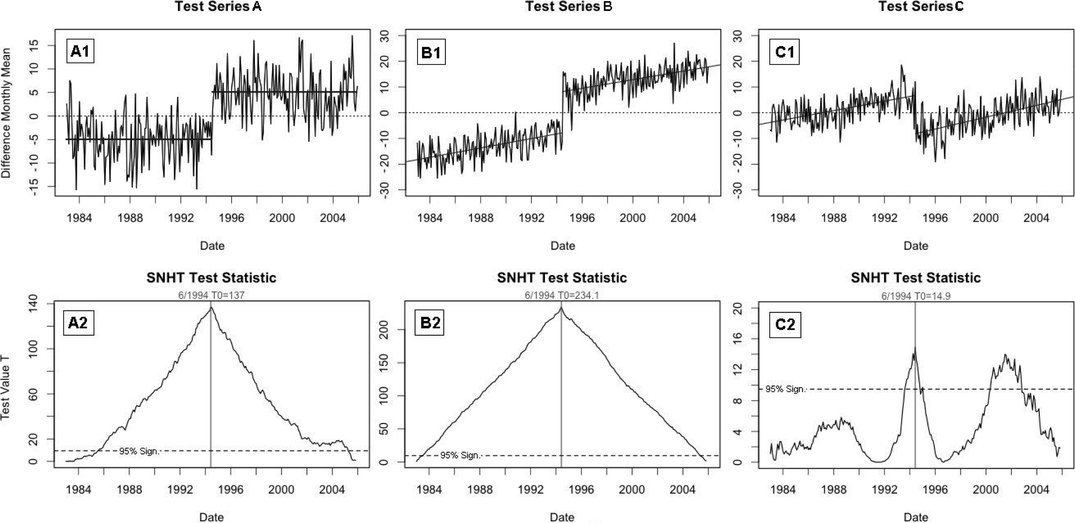
4.1. Single-Break Detection

In most of the analyses, we focused on the Standard Normal Homogeneity Test (SNHT, Alexandersson [35]) to detect possible discontinuities in the investigated time series. For each point, k, between one and n, with n being the length of the time series Y_i, i = 1,..., n, the test value, T (k), is calculated as follows:

$$T(k)=k{\overline{z}}_1^2+(n-k){\overline{z}}_2^2\hspace{0.17em}\hspace{0.17em}\hspace{0.17em}\hspace{0.17em}k=1,\dots ,n$$

(4)

with:

$${\overline{z}}_1=\frac{1}{k}\sum _{i=1}^k\left(Y_i-\overline{Y}\right)/s\hspace{0.17em}\hspace{0.17em}\hspace{0.17em};\hspace{0.17em}\hspace{0.17em}\hspace{0.17em}{\overline{z}}_2=\frac{1}{n-k}\sum _{i=k+1}^n\left(Y_i-\overline{Y}\right)/s$$

(5)

whereas Ȳ and s denote the mean and the standard deviation, respectively, over the whole time period. This calculation compares the standardized mean of the first k years (z̄₁) with that of the following n − k years (z̄₂). Large differences between the two mean values, indicating a shift of the mean at k, lead to high values of T (k). If the maximum of T (k) (denoted T₀) exceeds a certain level, T_c, a break point at the corresponding time is detected. The critical level, T_c, depends on the length of the investigated time series and the chosen significance level. Here, the T_c were derived using Monte Carlo simulations (random time series with normal distribution of the data). For example, the T_c at the significance level of 95% corresponds to the 95% quantile of the resulting distribution of T₀ (see the details in Alexandersson and Moberg [36]). Our T_c values, determined for the exact number of time steps used in the present analysis, are comparable to previously published values, e.g., [36]. It should be noted that the test statistics for T₀ show a strong sensitivity to the presence of trends. Using random time series with a variance comparable to those determined for the five BSRN reference time series and adding linear trends of 0.25 and 0.5 W·m⁻²·yr⁻¹ (as typical magnitudes for these series), respectively, the T_c at a 95% significance increased considerably, from 9 to 16 and 26, respectively. A similar degree of sensitivity is also found for the other test methods used in this work. In consequence, even the smallest trends in a time series tend to be detected as inhomogeneity. This is an important issue for break detection, especially when time series are tested without using reference series.

Ideally, the SNHT should be applied to the candidate time series only in comparison with a related reference time series of high quality. Here, we have considered time series of the difference (candidate minus a reference) for all investigated SIS data. This procedure will be referred to as relative homogeneity testing in the following. If the reference time series itself includes inhomogeneities, these will be detected in addition to the targeted ones in the investigated time series. To identify such problems, an absolute testing, thus a separate analysis of candidate and reference series, was also carried out. For all tests, monthly anomalies were used instead of the absolute SIS values, in order to eliminate the variability induced by the annual solar cycle and to remove possible seasonal difference patterns.

Figure 1 (panels A) illustrates the SNHT test for an artificial time series with a shift of the mean value at 06/1994. The test value, T, peaks at this date with a value of 137, which is far above the critical level of around 10 determined for the given length of this time series and a significance level of 95 %. The break detection is limited by the variability of the time series. If the magnitude of the shift is small compared to this variability, break detection may be imprecise (indicating slightly deviating dates of change) or may fail completely. As mentioned above, time series exhibiting a trend (which can be either natural or artificial) tend to be interpreted as inhomogeneous by the tests. However, in this case, the curve of the test statistic, T, is more plateau-like rather than showing a sharp maxima. Panels B and C of Figure 1 illustrate how the break detection is influenced by the presence of trends: An equidirectional trend leads to an overly pronounced test statistics; an antagonistic trend tends to mask the break.

Therefore, it can be helpful to remove trends prior to homogeneity testing, if only break-like inhomogeneities are of interest. However, a possible break itself imposes a trend, and thus, detrending can influence the test sensitivity. Nevertheless, we applied prior detrending as a complementary strategy for the field analyses presented in Section 6, assuming that in most of the areas, potential artificial shifts are small compared to underlying trends.

In order to enhance the confidence in the break identification, we also tested two further methods for the change point detection in a time series: the Buishand range test [37] and the Pettitt test [38]. A short description of these tests is given in the Appendix. All three tests showed highly consistent results. Discrepancies occurred mainly due to the fact that the SNHT is very sensitive to breaks near the beginning and the end of time series, while the other two methods are more sensitive to shifts in the middle of a time series [39]. Therefore, for most of the analyses presented in the following sections, we rely on the SNHT, while excluding positive results for the first and the last ten months of a time series to take into account the mentioned sensitivity problem of this method.

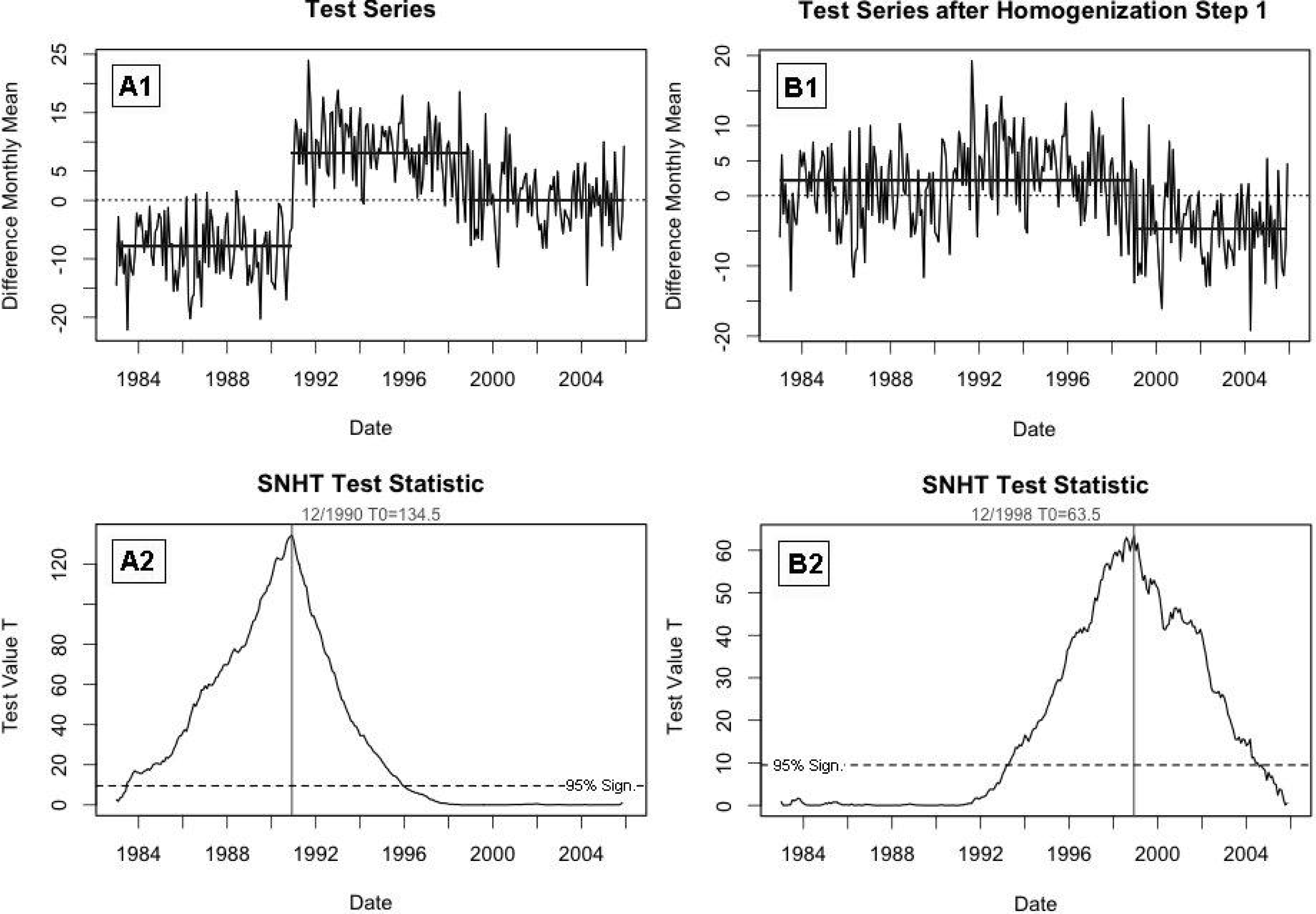
4.2. Multiple Break Detection

Observations from six different MVIRI instruments have been used to derive the SIS dataset. Hence, it is possible that multiple break points appear within the investigated time series.

To detect multiple breaks in the time series, the aforementioned test procedure has to be extended. The authors of Easterling and Peterson [40] described a method to homogenize climatological time series in consideration of multiple shifts by dividing the original time series into homogenous sub-series using the SNHT. Here, we apply a slightly different method that ensures a constant length of the analyzed time intervals and, therefore, allows the application of a fixed critical value for the test statistics. When the SNHT detects a break point in a time series, the two sub-series (before and after the break) are adjusted to means of zero (note that standardized time series are considered, Equation (5)). The corrected time series is subsequently tested again, and all significant breaks (dates and magnitudes) are recorded.

Figure 2 illustrates the first two steps of the described test method for a synthetic time series with two breaks (after 96 and 192 months). The dates of the two breaks are well detected. One drawback of this approach is the potentially imprecise adjustment of the two subseries in the homogenization steps, due to the presence of the so far undetected break points. Therefore, the magnitude of the break may not be correctly determined in the first step, and the adjustment may not be sufficient to completely remove the discontinuity in the corrected time series. However, the repeated detection of breaks in the following test steps allows for the detection of the same break point multiple times. The magnitudes of the detected shift for the same point in time are added up (even if the significance level is not reached again); thus, the error in the final break magnitude is expected to be small.

5. Analyses of Reference Data

In the first step, we investigated the homogeneity of the time series used as a reference in the analysis of the satellite-derived surface radiation dataset. The results of these analyses are presented in the following.

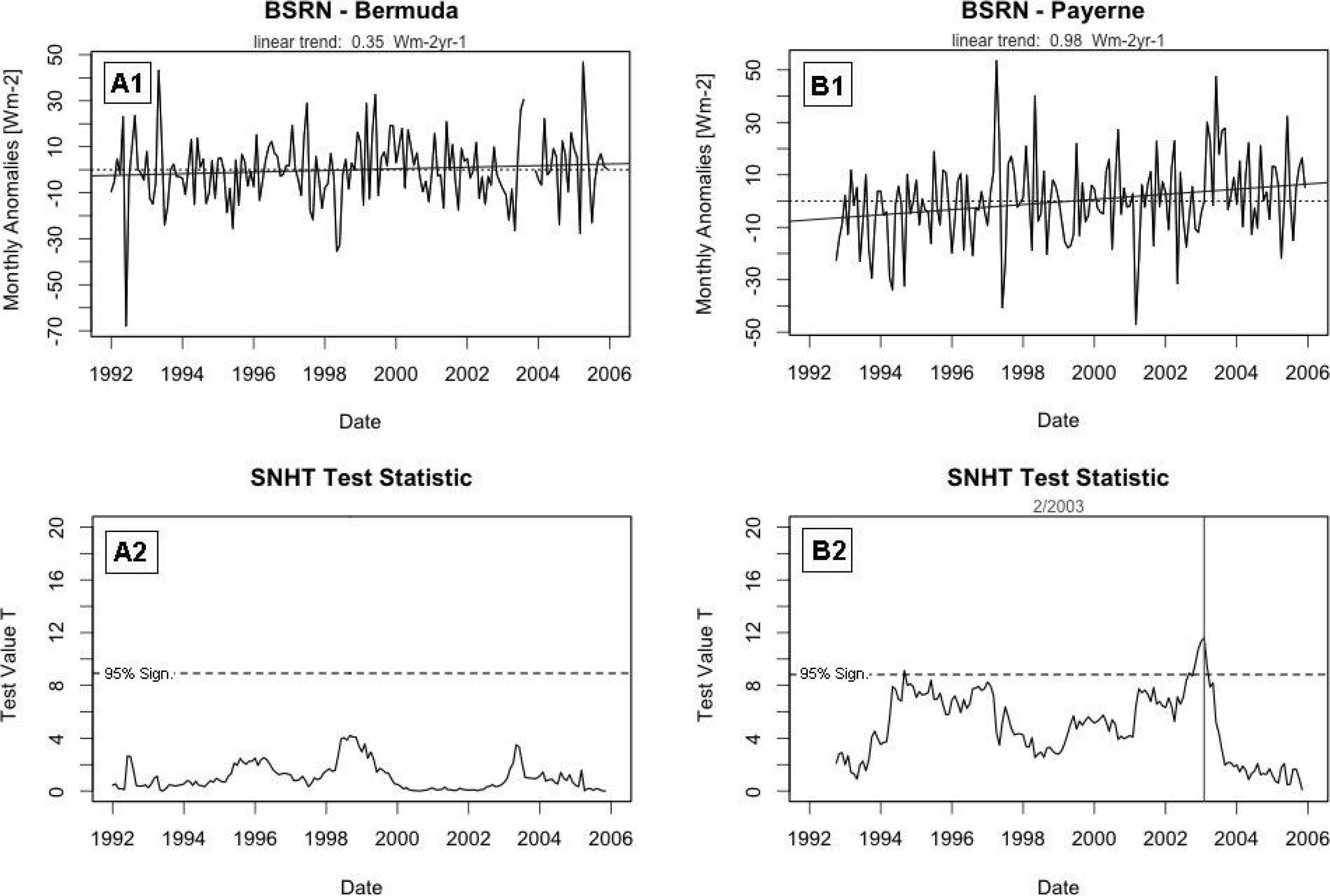
5.1. BSRN Measurements

The outcomes of the absolute homogeneity analyses for the BSRN surface radiation data are listed in

Table 2. Results of absolute homogeneity testing of BSRN station measurements (Carpentras (CAR), Florianopolis (FLO), Bermuda (BER), Lindenberg (LIN), Payerne (PAY)) and comparison with Alpine Surface Radiation Budget (ASRB) measurements at Payerne (last two columns).

Station	CAR	FLO	BER	LIN	PAY	PAY ASRB	ASRB vs. BSRN
Start Date	9/1996	7/1994	1/1992	10/1994	10/1992	1/1995	1/1995
SNHT:
T0/Tc	3.44/8.53	2.65/8.71	3.39/8.92	6.52/8.69	11.61/8.82	8.16/8.67	8.90/8.67
Date of Break					2/2003	(2/2003)	5/1996
Buishand:
R/Rc	1.04/1.62	1.32/1.63	1.06/1.63	1.48/1.63	1.39/1.63	1.29/1.63	1.03/1.63
Date of Break					(2/2003)	(2/2003)	(5/1996)
Pettitt:
Xk0/Xc	617/887	700/1,220	1,067/1,649	1,088/1,190	1,582/1,520	1,080/1,147	1,201/1,147
Date of Break					1/2003	(2/2003)	5/1996
Linear Trend
[W·m−2·yr−1]	0.59 ± 0.92	0.31 ± 0.87	0.23 ± 0.54	0.37 ± 0.82	0.98 ± 0.62	0.71 ± 0.84	0.06 ± 0.08

. Shown are the maximum test values, T₀ (SNHT), R (Buishand) and X_k0 (Pettitt), the corresponding critical values for a significance level of 95% and the linear trends of the time series of the monthly anomalies. In addition, for two of the stations, Bermuda and Payerne, the SNHT test statistics are shown (Figure 3). Four out of the five investigated time series are found to be homogeneous according to all three homogeneity tests, providing evidence of the good quality of the surface measurements. For the BSRN data from Payerne, the SNHT and the Pettitt test detect a break point in the first months of 2003 (compare Figure 3). It seems that several small breaks or, more likely, relative trends (note the linear trend of 0.98 ± 0.62 W·m⁻²·yr⁻¹ and the plateau-like maximum of the test statistics) favor a positive test result. The detection of trends as inhomogeneities highlights the difficulty of interpreting the result of absolute homogeneity testing and the importance of applying the test procedures to difference time series (in a relative testing).

To test whether the detected inhomogeneity in the BSRN surface measurements from Payerne is artificial or caused by natural variability, data from another surface measurement station in Payerne were analyzed. Since 1995, the Alpine Surface Radiation Budget (ASRB) project has been collecting data of the surface radiation budget in Payerne, very close to the measurement site of the BSRN station. The monthly averages of the surface downwelling solar radiation from the ASRB station and the difference of the monthly anomalies of the two time series from Payerne were analyzed in the same manner as above for the BSRN stations (Table 2).

The absolute tests detect the same dates of the maxima in the test statistics for the ASRB and the BSRN times series in Payerne. This suggests that the trend detected in the BSRN Payerne data is very likely not artificial. The relative analysis (ASRB vs. BSRN) shows very good agreement between the two measurement series, with a mean absolute bias of only 0.93 W·m⁻². Nevertheless, critical levels are reached for the Pettitt and the SNHT test at 05/1996, which is mainly due to unsystematic discrepancies up to 5 W·m⁻² (roughly within the measurement accuracy) occurring in very few months between 1996 and 1998. A significant inhomogeneity is thus not indicated for this BSRN SIS data record.

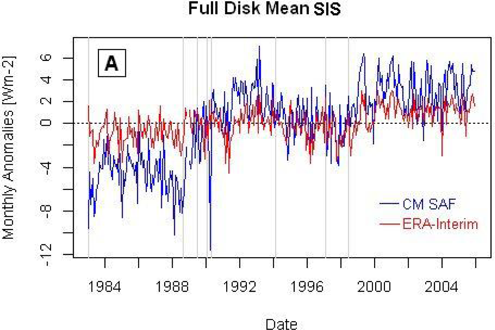
5.2. ERA-Interim Data

The solar surface radiation dataset from the ERA-Interim reanalysis was tested for homogeneity using all three test methods at each grid point. The results from the different procedures were found to be very consistent. Thus, we focus here on the SNHT results.

Figure 4A shows the SNHT test value, T₀, of the first analysis step wherever it exceeds the critical level. For most grid points, the time series are shown to be homogeneous. Only in some tropical regions, T₀ reaches significant values of up to 80. In panel B of the same figure, the numbers of independent inhomogeneities (identical dates are counted only once) for every grid point are illustrated. It is worth mentioning that the largest number of break points (up to six break points are detected for time series in the tropical Atlantic and in the north of Brazil) do not coincide with the regions of highest T₀ values. To assess the types of these inhomogeneities, we analyzed the time series from specific grid points in these tropical regions (not shown here). For the two regions with very high T₀ values over Africa, very broad maxima of T were found, which indicates the presence of significant long-term trends in the time series. In contrast, the test statistics for time series from the two regions with the highest number of inhomogeneities show relatively sharp peaks as a result of consecutive break-like inhomogeneities. However, a closer inspection of the time series shows that also these inhomogeneities occur over a period of several months and not by a sudden shift of the mean.

Figure 4C shows the frequency distribution of the detected inhomogeneities with respect to the date of their appearance. The distribution is found to be relatively uniform, without exhibiting single outstanding dates, indicating that no shifts are present on a global scale.

Additionally, a relative analysis of the ERA-Interim time series at BSRN sites was carried out. The results are shown in

Table 3. Results of the relative homogeneity tests of the time series from the ERA-Interim dataset at the grid points nearest to corresponding BSRN surface stations. Also given are mean absolute bias and the linear trend of the difference time series.

Station	CAR	FLO	BER	LIN	PAY	PAY ASRB
Start Date	9/1996	7/1994	1/1992	10/1994	10/1992	1/1995
SNHT:
T0/Tc	7.53/8.53	12.55/8.71	1.04/8.92	3.55/8.67	5.00/8.82	2.95/8.67
Date of Break		5/1999
Buishand:
R/Rc	1.21/1.62	2.21/1.63	0.83/1.63	1.11/1.63	1.34/1.63	1.28/1.63
Date of Break		5/1999
Pettitt:
Xk0/Xc	641/887	1,625/1,220	551/1,649	442/1,132	1,310/1,520	677/1,147
Date of Break		5/1999
Mean Bias
W·m−2	4.4	8.6	7.1	5.0	7.4	7.3
Linear Trend
[W·m−2·yr−1]	−0.30 ± 0.40	0.58 ± 0.56	0.00 ± 0.35	0.03 ± 0.37	−0.26 ± 0.39	0.00 ± 0.50

. Due to the significant scale differences in this comparison (the ERA-Interim data represent spatially averaged information over an area of about 80 × 80 km), a break detection tends to be suppressed by a relatively high variation of the difference time series. Thus, the test results of this experiment only give rough information on the homogeneity of ERA-Interim. Nevertheless, we find an acceptable agreement between the datasets. The mean absolute bias between the datasets is in the order of the accuracy of the surface observations. Only for the data from Florianopolis (Brazil, 48.5°W, 27.5°S), an inhomogeneity is detected by all three test methods, as a result of a significant positive trend in the difference time series.

Consistent with the findings from Section 5.1, no artificial inhomogeneity is detected according to the relative homogeneity analysis at Payerne (Switzerland, 6.9°E, 46.8°N). The positive trend present in all three reference series (BSRN, ASRB and ERA-Interim) at this site tends to be interpreted as an inhomogeneity in an absolute analysis.

5.3. Discussion

The homogeneity analysis of the BSRN observations indicates their suitability as reference data records for the analysis of the satellite-derived SIS. The positive trend in BSRN SIS at station Payerne represents an atmospheric effect rather than an artificial inhomogeneity.

The absolute analysis of the ERA-Interim dataset for the full disk covered by the satellite data shows a high degree of homogeneity of the data for most regions. However, in a few tropical areas, clear inhomogeneities in the time series are detected. In other areas, the test statistics show values slightly above the significance level. Whether these inhomogeneities are associated with atmospheric effects (e.g., trends) or introduced artificially cannot be decided without the application of a primary reference dataset. From the comparison with the BSRN surface observations, an indication for both atmospheric and artificial changes is given. As will be discussed in the next section, we combine the information from absolute and relative analysis in the testing of the CM SAF data, in order to avoid an inhomogeneity detection as a result of inconsistent ERA-Interim data.

6. Analyses of the CM SAF SIS Data Record

In this section, the homogeneity investigation of the satellite-derived SIS data record using absolute and relative homogeneity testing is presented.

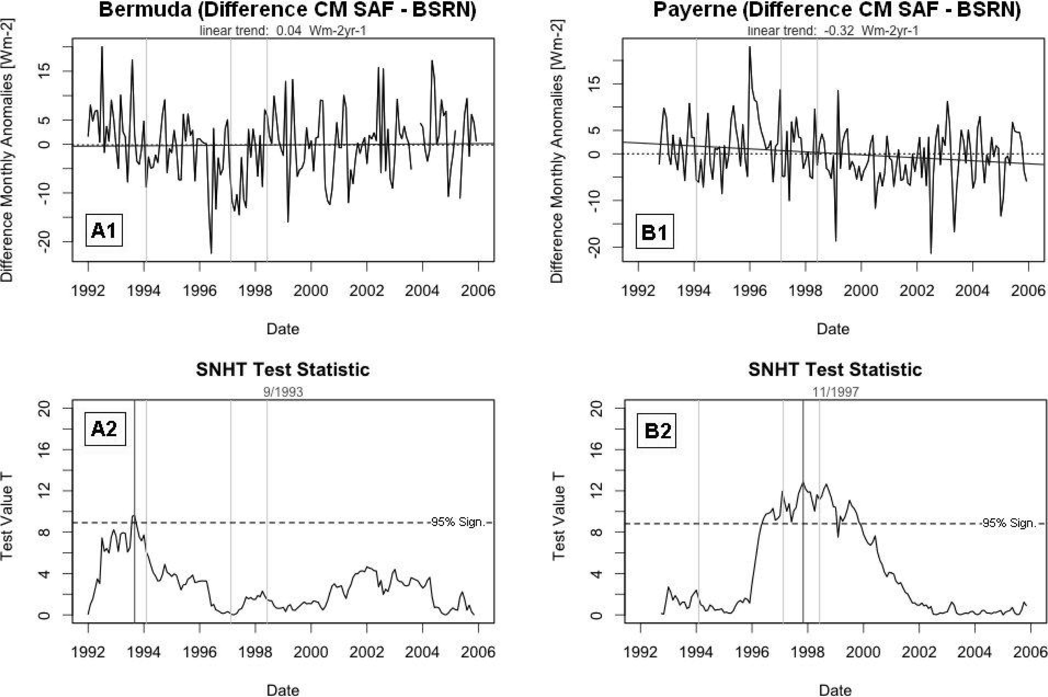
6.1. Analyses at BSRN Sites

To assess the homogeneity of the CM SAF dataset at the sites of the BSRN stations, absolute analyses of the candidate series and relative analyses versus the corresponding surface reference time series were conducted. The results of these analyses are summarized in

Table 4. Results of the absolute homogeneity testing of the CM SAF SIS dataset at the grid points nearest to the corresponding BSRN stations.

Station	CAR	FLO	BER	LIN	PAY
Start Date	9/1996	7/1994	1/1992	10/1994	10/1992
SNHT:
T0/Tc	4.78/8.53	2.56/8.71	5.44/8.92	7.67/8.69	8.12/8.82
Date of Break					(1/2003)
Buishand:
R/Rc	1.12/1.62	1.25/1.63	1.54/1.63	1.57/1.63	1.18/1.63
Date of Break					(1/2003)
Pettitt:
Xk0/Xc	742/887	607/1,220	1,485/1,649	1,156/1,190	1,268/1,520
Date of Break					(1/2003)
Linear Trend
[W· m−2· yr−1]	0.81 ± 0.99	0.29 ± 0.88	0.31 ± 0.56	0.55 ± 0.86	0.66 ± 0.70

and

Table 5. As in Table 4, but a relative analysis (compared to corresponding BSRN surface measurements).

Station	CAR	FLO	BER	LIN	PAY BSRN	PAY ASRB
Start Date	9/1996	7/1994	1/1992	10/1994	10/1992	1/1995
SNHT:
T0/Tc	12.47/8.53	2.25/8.71	9.61/8.92	7.47/8.69	12.86/8.82	15.64/8.67
Date of Break	8/2004		9/1993	(4/2002)	11/1997	2/1997
Buishand:
R/Rc	1.45/1.62	1.11/1.63	1.92/1.63	1.52/1.63	1.94/1.63	1.92/1.63
Date of Break	(1/2003)		9/1993	(4/2002)	9/1998	9/1998
Pettitt:
Xk0/Xc	809/887	649/1,220	1,327/1,649	1,414/1,190	1,882/1,520	1,461/1,147
Date of Break	(1/2003)		(9/1993)	4/2002	9/1998	9/1998
Mean Bias
[W· m−2]	2.9	6.1	5.3	3.0	4.8	4.9
Linear Trend
W·m−2·yr−1	0.22 ± 0.26	−0.03 ± 0.42	0.04 ± 0.27	0.18 ± 0.21	−0.32 ± 0.25	−0.48 ± 0.34

.

Based on the absolute analyses, all five CM SAF time series are found to be homogeneous according to the three test procedures (Table 4). For consistency reasons, the same limited time periods as available for the reference time series were considered. The relative homogeneity analyses with the BSRN reference, however, reveal inhomogeneities indicated by one or two tests for the time series from Carpentras, Bermuda and Lindenberg (Table 5). Furthermore, all three tests identify a significant inhomogeneity of CM SAF SIS at Payerne.

Figure 5 illustrates the results of the relative analyses at the sites Bermuda and Payerne. At Bermuda, the inhomogeneity detected by the SNHT and the Buishand test in September, 1993 (i.e., relatively close to the start of the time series), is caused by a slight negative trend around that year in the difference time series. In both cases, the test statistics only slightly exceeded the level of significance. A broad maximum in the test statistics between 1996 and 2000 indicates a significant relative trend at Payerne. In agreement with these findings, the inhomogeneities detected for the difference time series at Lindenberg and Carpentras (not shown) can also be attributed to gradual changes rather than to a sudden shift.

For Payerne, the satellite data show a positive trend over the considered time period; however, this trend is smaller and statistically less significant than the trend derived from the BSRN measurements in Payerne (0.66 W·m⁻²·yr⁻¹ (CM SAF) compared to 0.98 W·m⁻²·yr⁻¹ (BSRN); see Tables 2 and 4). The underestimation of the positive trend by CM SAF SIS might be caused by neglecting changes in aerosol optical depth in the retrieval of these data.

Overall, the absolute and the relative homogeneity tests of the CM SAF surface radiation data at the five sites underline the good quality of the dataset in the time period covered by BSRN data. Most importantly, none of the detected inhomogeneities at the investigated sites could be associated with changes in the satellite instruments. However, it should be reminded that no information can be drawn from this experiment for all satellite changes before 1992.

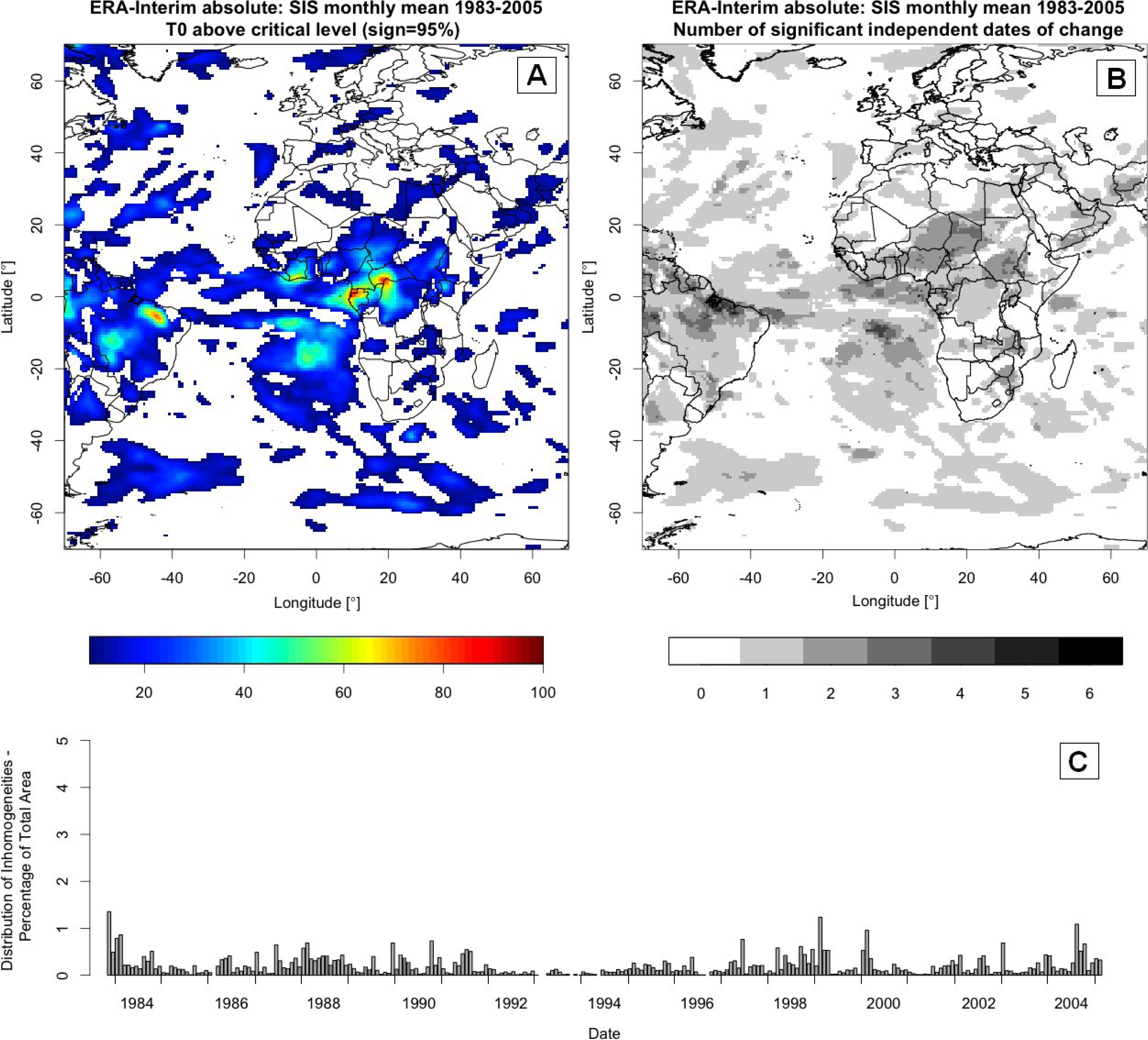
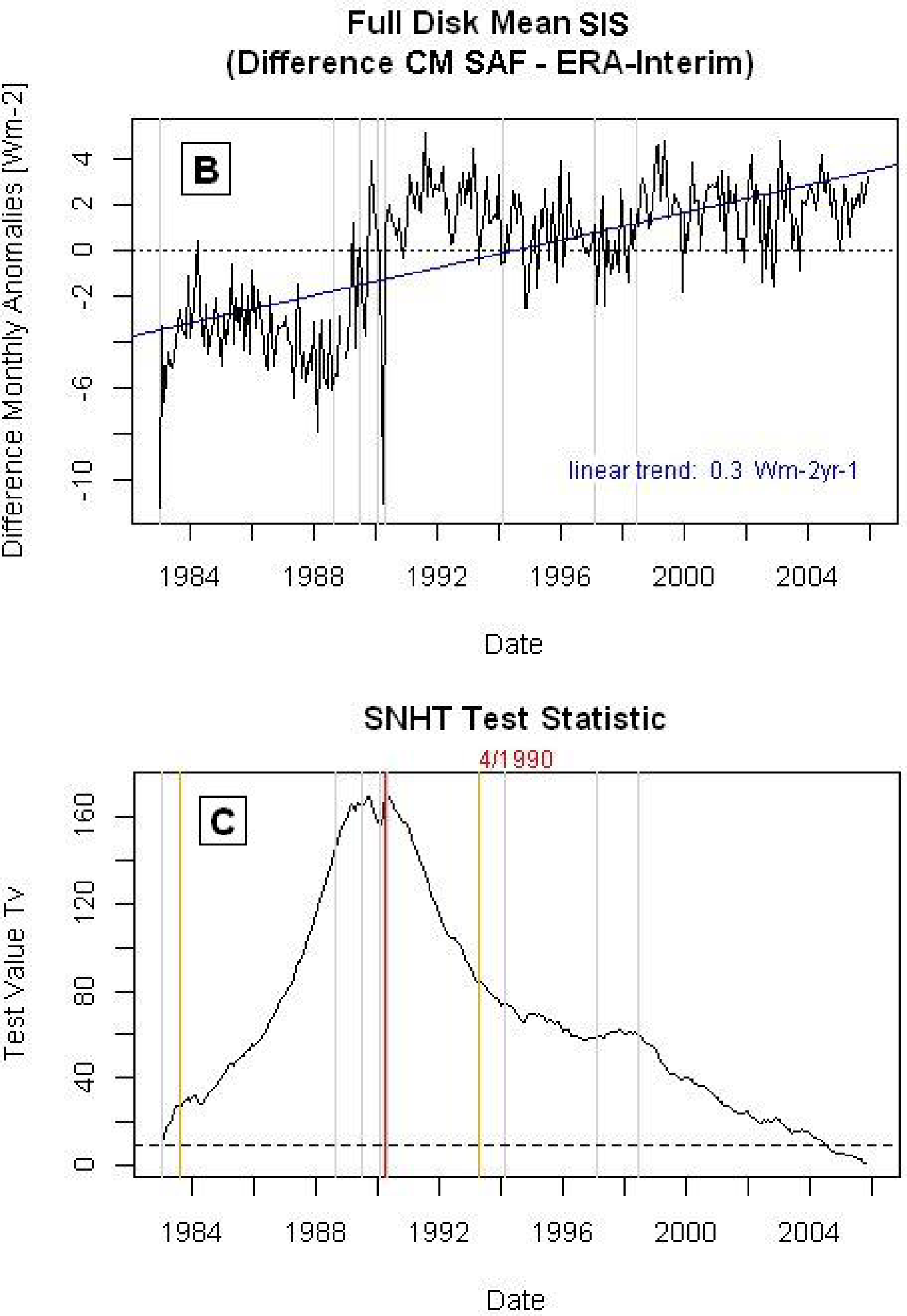
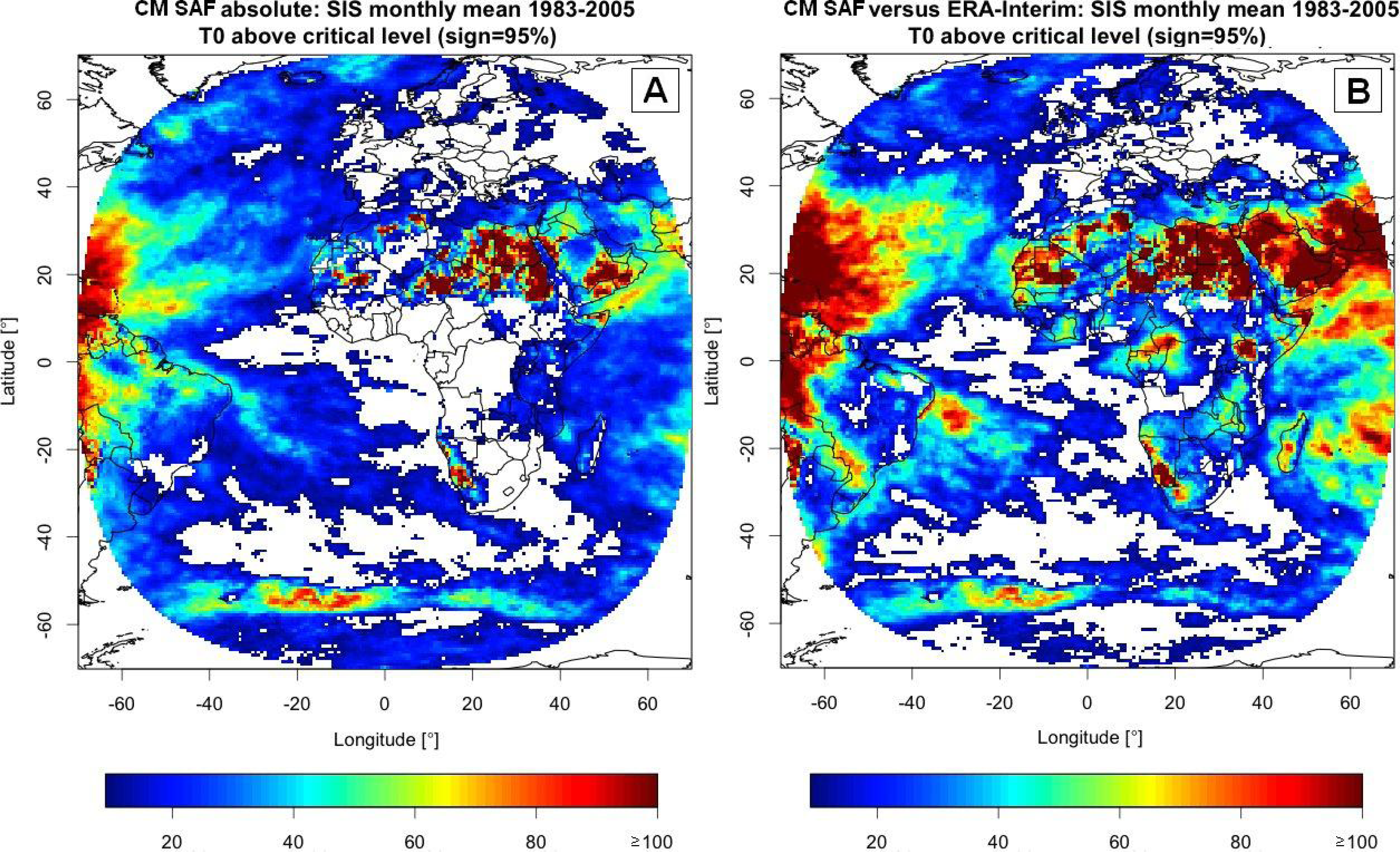
6.2. Full Domain Analyses

In the following, we present the analyses of CM SAF SIS in the full domain using absolute homogeneity testing and using relative testing with ERA-Interim data as the reference. For easier comparison, the CM SAF dataset was regridded onto the ERA-Interim spatial grid using first order conservative remapping. This remapping involves additional uncertainties. Due to the coarse resolution of the ERA-Interim model physics, systematic deviations between ERA-Interim and the spatially averaged CM SAF data could appear. As a consequence, the break detection could be suppressed by a relatively high variability of the difference time series, on the one hand. On the other hand, the spatial averaging also tends to reduce the temporal variability. Therefore, an analysis on such a coarse grid also has advantages, provided that breaks occur on the scale of the coarse grid or larger, which can be expected from satellite data.

In the first step, the spatial means over the full domain were calculated for both data fields (Figure 6A). Overall, variability and temporal trends of the CM SAF data are higher than for the corresponding data of ERA-Interim. The difference time series (Figure 6B) exhibits large changes. SNHT detects a clear break in CM SAF SIS for April 1990 (Figure 6C). This break occurs exactly on the date of an instrument change (corresponding dates are marked grey). Two further change points (marked orange), detected in subsequent analysis steps, do not coincide with any of these instrument changes. Nevertheless, additional artificial changes are apparent in the difference series, e.g., a strong gradual decrease appearing in the months before the break in April 1990.

In the next step, an absolute homogeneity analysis of the CM SAF data field was performed (for each grid point individually) using the same test procedures as in Section 5.2. In Figure 7A the results of these absolute analyses for the test value, T₀, as diagnosed for each grid point are shown. While over some regions (e.g., Europe), no inhomogeneities are detected in the dataset, in certain areas (especially in Africa) very large values of T₀ of up to around 200 are found. For most of these areas, multiple inhomogeneities (up to nine) are diagnosed (not shown).

The results of the relative analysis using the ERA-Interim dataset as the reference are shown in Figure 7B. As shown in Section 5.2, in a few regions, especially in the tropics, the ERA-Interim data contain considerable inhomogeneities. To address this issue, we consider in the following only those inhomogeneities detected by the relative analysis that are also found by the absolute homogeneity testing. In this way, we avoid the detection of break points that are likely associated with inhomogeneities in the ERA-Interim reference dataset.

These filtering conditions lead to a modified distribution of inhomogeneities. In Figure 8A,B, the test values, T₀, above the significance level and the number of detected inhomogeneities are shown. The grey shaded areas in A mark all filtered regions for which we cannot make a clear statement, as only the relative calculations indicate inconsistencies.

Areas with numerous inhomogeneities of very high significance are found, especially in some regions of North Africa, whereas the majority of the observation area is indicated to be homogeneous (e.g., continental Europe) or only slightly problematic (with one detected inhomogeneity, as found for many oceanic regions).

As noted before, the test methods used in this work are not able to distinguish between break- and trend-like inhomogeneities. In order to assess this aspect, three further analysis steps were carried out. Besides a visual inspection of the time series at single grid points, the frequency distribution of the detected dates of change is used to derive valuable information. Additionally, a detrended analysis, thus an inhomogeneity testing after removal of long-term linear trends from the tested time series, can help to separate the different types of inhomogeneities. The results of these analysis steps are presented in the following.

Figure 8C displays the frequency distribution of the dates of the inhomogeneities analyzed in the filtered relative calculations. The findings clearly indicate the presence of breaks associated with instrument changes (marked red) on a global scale. The largest impact is indicated for the change in 04/1990, which is detected as a break point in about 6 % of the total area. Further breaks caused by instrument changes occur for 05/1998, 02/1997 and 06/1989. A change of the SIS retrieval in October 1994 (Rebekka Posselt, personal communication), is also found to have an impact on the stability of the data in certain regions (see arrow in Figure 8C). For the time period between 1988 and 1990, the number of detected inhomogeneities is large, which could indicate the presence of significant trends in addition to single breaks. This observation refers to considerable instrumental problems on-board the Meteosat-3 generation (Richard Müller, personal communication) used mainly between August 1988 and June 1989, as well as from February to April 1990 (Table 1).

For two grid points with exceptionally high T₀ values, the analysis is illustrated in Figure 9. At the grid point in Sudan (panels A1 and A2), a strong break occurs at 05/1998 (marked red). This and at least two of the eight inhomogeneities (02/1997 and 10/1994) detected in the following analysis steps (marked orange) coincide with modifications in the measurements (marked grey). The second grid point in Niger (panels B1 and B2) shows a clear break for the instrument change in June, 1989. The other four inhomogeneities detected for this site are less pronounced and apparently not connected with further satellite changes. Nevertheless, for both series, additional trend-like inhomogeneities within single satellite periods can be observed. This finding indicates the presence of gradual changes related to sensitivity variations of the instruments, even though the retrieval method is supposed to correct such changes (compare Section 2).

In an extended analysis, all tested time series were detrended (by eliminating the linear trend over the whole period) before the homogeneity testing. As discussed in Section 4.1, the presence of long-term trends tends to mask or elevate the significance of breaks or short-term trends, depending on the signs of shifts and trends. On the other hand, the presence of shifts in time series can lead to an incorrect trend estimation and correction. Therefore, the following analysis should be considered only in conjunction with the investigations of the uncorrected time series.

The outcomes of the detrended calculations are displayed in Figure 10. The T₀ values (Figure 10A) are considerably lower compared to Figure 8 in most of the regions. In accordance with these results, the frequency of significant inhomogeneities is reduced for most of the dates (Figure 10C). These findings indicate the significant impact of long-term relative trends between the CM SAF and ERA-Interim data on the distribution of inhomogeneities. Many of the problematic regions are located near the edge of the observation area. This could be associated with the low observation angle of the satellites for these regions (see, also, the discussion in the next section).

Concerning the number of breaks at the individual grid points (panel B), the changes with respect to Figure 8 differ: while in some areas, the number of breaks is reduced (as for the highly problematic regions in Africa), other regions, especially over the oceans, now exhibit two breaks instead of one. It is possible that these additional breaks were partly hidden, due to the influence of long-term trends. The frequency distribution (panel C) shows that especially the breaks at 01/1994 and 10/1994 are more pronounced in this detrended analysis. Other breaks (e.g., 04/1990) are less frequent than before.

Figure 11 shows the regions with inhomogeneities (according to the detrended analysis) occurring at dates coinciding with at least one of the seven instrument changes or the retrieval modification in 10/1994. In panel A, the numbers of such breaks at the individual grid points are illustrated in grey colors. Up to four of the discontinuities detected at grid points in the highly problematic regions of Africa can be attributed to alterations in the satellite measurements. The three further panels of Figure 11 show the magnitudes of the shifts as determined for three of these changes with a large impact on the SIS data. For March/April 1990 (panel B), many regions over the land areas of North Africa, as well as some areas in the Atlantic and the Indian Ocean exhibit positive shifts below or around 10 W/m². These magnitudes seem to be small considering the outcomes for the full domain spatial mean time series (Figure 6). As could be seen in the same figure, a strong gradual decrease appears in the months before the positive shift in April, 1990; thus, detection and quantification of this break point are expected to be less precise. For October 1994 (panel C), negative breaks, partly exceeding 30 W/m², are found. The spatial distribution for this date is very consistent, no matter if detrending was used or not. Significant positive breaks occur for May 1998 (panel D). The two latter breaks, along with the breaks occurring in 01/1994 and 02/1997 (not shown in the figure), are spatially limited to the aforementioned highly problematic regions in Africa, e.g., Egypt, Sudan or Namibia. The mentioned areas typically exhibit mountainous land surfaces without significant vegetation. This point leads to the question of how these breaks in the satellite time series can be explained, which will be shortly discussed in the following section.

6.3. Possible Causes of Discontinuities

In areas with relatively bright surfaces (as found in problematic desert-like regions), the difference between the normalized counts, ρ_max and ρ_cs (see Equation (1)), is relatively small, which leads to a high dependency on changes in the instrument sensitivity. Relatively high determination errors of SIS also occur for regions towards the edge of the CM SAF SIS domain, as the relatively low observation angle involves uncertainties related with the increase of scattered light, an enlargement of the observation area per pixel and a decrease of the spatial representativeness (cloud and surface information increasingly mismatch).

Another important issue refers to the spectral sensitivity that slightly differs between the instrument generations used on Meteosat. This aspect has been investigated in [41]. The authors found significant deviations in the spectral response function for Meteosat 2, 3 and 4. Even though the Heliosat retrieval method does not explicitly correct for these changes, discontinuities in the final data should be avoided by the continuous adjustment of ρ_max and ρ_cs. Another problem lies in the fact that the relationship between cloud albedo n and SIS is not perfectly linear over the whole range. For this reason, more complex calculations of the clear-sky index, k, are applied for small and large values of n. If deviations in this respect occur from satellite to satellite, regions with very low cloud coverage (as is the case for the problematic regions detected in our study) or high cloud coverage are expected to be very sensitive to measurement changes.

7. Summary and Discussion

The homogeneity of the CM SAF SIS data for the period of 1983 to 2005 for the disk area ± 70° in latitude and longitude was investigated using three test methods. In the first step, the homogeneity of the station-based BSRN SIS and the ERA-Interim reanalysis SIS data series were investigated. The outcomes show that both data records are appropriate for usage as reference series in relative homogeneity testing. The CM SAF SIS show no break points or other clear inhomogeneities at the BSRN sites in the time periods available for BSRN (starting earliest in 1992), in conformity with preliminary investigations by [10].

The ERA-Interim record, available for the full period and the full CM SAF domain, was used for a more comprehensive investigation of the satellite data. These field analyses reveal substantial regional differences in the stability of the CM SAF record. For the majority of the regions (e.g., Europe) no shifts related to satellite changes are found. However, significant discrepancies between the satellite and the ERA-Interim data are indicated for many regions, especially towards the edge areas of the CM SAF domain. Numerous discontinuities occur in the time period between 1988 and 1990, when the problematic Meteosat-3 instrument generation apparently has caused breaks and artificial trends. Furthermore, for later instrument changes, inhomogeneities are found. For example, in confined areas in Africa, a multitude of satellite-related breaks is detected. These areas typically exhibit mountainous surfaces without significant vegetation, which refers to possible problems with the satellite measurements in combination with the data retrieval used for such specific surface conditions.

Nevertheless, satellite and retrieval changes are expected to have a global impact on the SIS data. Thus, similar breaks (but less pronounced and, therefore, possibly not detected against the natural SIS variability) might also occur in regions outside of the mentioned areas in Africa. This assumption is supported by [23], who found inhomogeneities in the CM SAF surface radiation dataset over Europe in the late 1980s and early 1990s using homogenized station datasets as the reference.

While most of the detected breaks can be well attributed to changes in the instrumentation, the relative trends observed between the CM SAF SIS and the reference SIS records are not necessarily a result of the inaccuracy of satellite measurements. Such gradual changes, especially with respect to surface measurements, might also be introduced by the direct aerosol effect on SIS, as this direct impact by changing aerosol abundances would be included in the surface time series, but not in the satellite series based on cloud albedo measurements and with the assumption of a constant aerosol climatology.

8. Conclusions

Overall, our study shows that the surface solar irradiance (SIS) dataset provided by the EUMETSAT Satellite Application Facility on Climate Monitoring (CM SAF) compares well with prominent reference data. However, its use for climate trend analysis can only be recommended for certain regions and time frames, as artificial breaks as a result of instrument changes have been detected in certain areas. In many regions, e.g., Europe, significant breaks have not been found in our investigations, but small discontinuities potentially affecting trend analysis cannot also be excluded for these regions.

In conclusion, we suggest a further and more specific assessment of this data record and the application of homogenization techniques aiming at the correction of artificial changes, as identified in this study. The first efforts have been made in this respect in a recently published follow-up study by [42]. Furthermore, the results of our study may help to identify and solve possible shortcomings in the retrieval algorithm of this dataset.

References

1. IPCC. Climate Change 2007: The Physical Science Basis. Contribution of Working Group I to the Fourth Assessment Report of the Intergovernmental Panel on Climate Change; Cambridge University Press: Cambridge, UK, 2007. [Google Scholar]
2. Ohmura, A. Observed decadal variations in surface solar radiation and their causes. J. Geophys. Res 2009, 114, D00D05. [Google Scholar]
3. Ohmura, A.; Gilgen, H.; Hegner, H.; Mller, G.; Wild, M. Baseline Surface Radiation Network (BSRN/WCRP): New Precision Radiometry for Climate Research. Bull. Am. Meteorol. Soc 1998, 79, 2115–2136. [Google Scholar]
4. Wild, M. Global dimming and brightening: A review. J. Geophys. Res 2009, 114, D00D16. [Google Scholar]
5. Wild, M. Enlightening global dimming and brightening. Bull. Am. Meteorol. Soc 2012, 93, 27–37. [Google Scholar]
6. Cermak, J.; Wild, M.; Knutti, R.; Mishchenko, M.I.; Heidinger, A.K. Consistency of global satellite-derived aerosol and cloud data sets with recent brightening observations. Geophys. Res. Lett 2010, 37, L21704. [Google Scholar]
7. Norris, J.R.; Wild, M. Trends in aerosol radiative effects over Europe inferred from observed cloud cover, solar “dimming,” and solar “brightening”. J. Geophys. Res 2007, 112, D08214. [Google Scholar]
8. Müller, R.W.; Matsoukas, C.; Gratzki, A.; Behr, H.D.; Hollmann, R. The CM-SAF operational scheme for the satellite based retrieval of solar surface irradiance—ALUT based eigenvector hybrid approach. Remote Sens. Environ 2009, 113, 1012–1024. [Google Scholar]
9. Pinker, R.T.; Laszlo, I. Modeling surface solar irradiance for satellite applications on a global scale. J. Appl. Meteorol 1992, 31, 194–211. [Google Scholar]
10. Posselt, R.; Mueller, R.; Stöckli, R.; Trentmann, J. Remote sensing of solar surface radiation for climate monitoring—the CM-SAF retrieval in international comparison. Remote Sens. Environ 2012, 118, 186–198. [Google Scholar]
11. Wang, H.; Pinker, R.T. Shortwave radiative fluxes from MODIS: Model development and implementation. J. Geophys. Res 2009, 114, D20201. [Google Scholar]
12. Zhang, Y.-C.; Rossow, W.B.; Lacis, A.A. Calculation of surface and top of atmosphere radiative fluxes from physical quantities based on ISCCP data sets 1. Method and sensitivity to input data uncertainties. J. Geophys. Res 1995, 100, 1149–1165. [Google Scholar]
13. Zhang, Y.; Rossow, W.B.; Lacis, A.A.; Oinas, V.; Mishchenko, M.I. Calculation of radiative fluxes from the surface to top of atmosphere based on ISCCP and other global data sets: Refinements of the radiative transfer model and the input data. J. Geophys. Res 2004, 109, D19105. [Google Scholar]
14. Stackhouse, P.W., Jr.; Gupta, S.K.; Cox, S.; Zhang, T.; Mikovitz, J.C.; Hinkelman, L.M. 24.5-year SRB data set released. GEWEX News 2011, 21, 10–12. [Google Scholar]
15. Rossow, W.B.; Schiffer, R. Advances in understanding clouds from ISCCP. Bull. Am. Meteorol. Soc 1999, 80, 2261–2287. [Google Scholar]
16. Peterson, T.C.; Easterling, D.R.; Karl, T.R.; Groisman, P.; Nicholls, N.; Plummer, N.; Torok, S.; Auer, I.; Boehm, R.; Gullett, D.; et al. Homogeneity adjustments of in situ atmospheric climate data: A review. Int. J. Climatol 1998, 18, 1493–1517. [Google Scholar]
17. Reeves, J.; Chena, J.; Wang, X.L.; Lund, R.; Lu, Q. A review and comparison of changepoint detection techniques for climate data. J. Appl. Meteorol. Clim 2007, 46, 900–915. [Google Scholar]
18. Venema, V.K.C.; Mestre, O.; Aguilar, E.; Auer, I.; Guijarro, J.A.; Domonkos, P.; Vertacnik, G.; Szentimrey, T.; Stepanek, P.; Zahradnicek, P.; et al. Benchmarking homogenization algorithms for monthly data. Clim. Past 2012, 8, 89–115. [Google Scholar]
19. Wijngaard, J.B.; Tank, A.M.G.K.; Können, G.P. Homogeneity of the 20th century European daily temperature and precipitation series. Int. J. Climatol 2003, 23, 679–692. [Google Scholar]
20. Moberg, A.; Alexandersson, H. Homogenization of swedish temperature data. part I: Homogenized gridded air temperature compared with a subset of global gridded air temperature since 1861. Int. J. Climatol 1997, 17, 35–54. [Google Scholar]
21. Guentchev, G.; Barsugli, J.J.; Eischeid, J. Homogeneity of gridded precipitation datasets for the Colorado river basin. J. Appl. Meteorol. Clim 2010, 49, 2404–2415. [Google Scholar]
22. Ferguson, C.; Villarini, G. Detecting inhomogeneities in the twentieth century reanalysis over the central United States. J. Geophys. Res 2012, 117, D05123. [Google Scholar]
23. Sanchez-Lorenzo, A.; Wild, M.; Trentmann, J. Validation and stability assessment of the monthly mean CM SAF surface solar radiation data set over Europe against a homogenized surface dataset (1983–2005). Remote Sens. Environ 2013, 134, 355–366. [Google Scholar]
24. Gilgen, H.; Wild, M.; Ohmura, A. Means and trends of shortwave irradiance at the surface estimated from GEBA. J. Clim 1998, 11, 2042–2061. [Google Scholar]
25. Beyer, H.G.; Costanzo, C.; Heinemann, D. Modifications of the Heliosat procedure for irradiance estimates from satellite images. Solar Energy 1996, 56, 207–212. [Google Scholar]
26. Cano, D.; Monget, J.M.; Albuisson, M.; Guillard, H.; Regas, N.; Wald, L. A method for the determination of the global solar radiation from meteorological satellite data. Solar Energy 1986, 37, 31–39. [Google Scholar]
27. Hammer, A.; Heinemanna, D.; Hoyer, C.; Kuhlemann, R.; Lorenz, E.; Müller, R.; Beyer, H.G. Solar energy assessment using remote sensing technologies. Remote Sens. Environ 2003, 86, 423–432. [Google Scholar]
28. Rigollier, C.; Lefèvre, M.; Wald, L. The method Heliosat-2 for deriving shortwave solar radiation from satellite images. Solar Energy 2004, 77, 159–169. [Google Scholar]
29. Diekmann, F.-J.; Happ, S.; Rieland, M.; Benesch, W.; Czeplak, G.; Kasten, F. An operational estimate of global solar irradiance at ground level from METEOSAT data: Results from 1985 to 1987. Meteorol. Rdsch 1988, 41, 65–79. [Google Scholar]
30. Rigollier, C.; Lefèvre, M.; Blanc, P.; Wald, L. The operational calibration of images taken in the visible channel of the meteosat series of satellites. J. Atmos. Ocean. Technol 2002, 19, 1285–1293. [Google Scholar]
31. Raschke, E.; Kinne, S.; Stackhouse, P.W. Gewex Radiative Flux Assessment (rfa); WCRP Report No. 19/2012.2012. World Climate Research Programme (WCRP): Geneva, Switzerland, 2012. Available online: http://www.wcrp-climate.org/documents/GEWEX%20RFA-Volume%201-report.pdf (accessed on 20 December 2013).
32. Roesch, A.; Wild, M.; Ohmura, A.; Dutton, E.G.; Long, C.N.; Zhang, T. Assessment of BSRN radiation records for the computation of monthly means. Atmos. Meas. Tech 2011, 4, 339–354. [Google Scholar] [Green Version]
33. Dee, D.P.; Uppala, S.M.; Simmons, A.J.; Berrisford, P.; Poli, P.; Kobayashi, S.; Andrae, U.; Balmaseda, M.A.; Balsamo, G.; Bauer, P. The ERA-Interim reanalysis: Configuration and performance of the data assimilation system. Q. J. R. Meteorol. Soc 2011, 137, 553–597. [Google Scholar]
34. Simmons, A.J.; Willett, K.M.; Jones, P.; Thorne, P.W.; Dee, D.P. Low-frequency variations in surface atmospheric humidity, temperature, and precipitation: Inferences from reanalyses and monthly gridded observational data sets. J. Geophys. Res.: Atmos 2010, 115, D01110. [Google Scholar]
35. Alexandersson, H. A homogeneity test applied to precipitation data. Int. J. Climatol 1986, 6, 661–675. [Google Scholar]
36. Alexandersson, H.; Moberg, A. Homogenization of swedish temperature data. part I: Homogeneity test for linear trends. Int. J. Climatol 1997, 17, 25–34. [Google Scholar]
37. Buishand, T. Some methods for testing the homogeneity of rainfall records. J. Hydrol 1982, 58, 11–27. [Google Scholar]
38. Pettitt, A.N. A non-parametric approach to the change-point problem. Appl. Stat 1979, 28, 126–135. [Google Scholar]
39. Hawkins, D.M. Testing a sequence of observations for a shift in location. J. Am. Stat. Assoc 1977, 72, 180–186. [Google Scholar]
40. Easterling, D.R.; Peterson, T.C. A new method for detecting undocumented discontinuities in climatological time series. Int. J. Climatol 1995, 15, 369–377. [Google Scholar]
41. Govaerts, Y.M.; Clerici, M.; Clerbaux, N. Operational calibration of the meteosat radiometer VIS band. IEEE Trans. Geosci. Remote Sens 2004, 42, 1900–1914. [Google Scholar]
42. Krähenmann, S.; Obregon, A.; Müller, R.; Trentmann, J.; Ahrens, B. A satellite-based surface radiation climatology derived by combining climate data records and near-real-time data. Remote Sens 2013, 5, 4693–4718. [Google Scholar]
Appendix A. Test Procedures
A.1. Buishand Range Test
The Buishand range test [37] considers the partial sums, S k *, which describe the cumulative deviations from the mean of the time series.
S k * = i = 1 k ( Y i Y ¯ ) k = 1 , , n
For a homogeneous series without a trend, S k * is expected to fluctuate around zero. In the case of a break at date k0, S k * will show an extremum around this date. Significance is given, if the “rescaled adjusted range”, R, defining the difference between the minimum and maximum of S k * (normalized to the standard deviation, s, of the data), exceeds a certain level.
R = ( max S k * min S k * ) / s
The critical values, Rc (as shown in tables 2 and 5), are derived using Monte Carlo simulations (see Section 4.1).
A.2. Pettitt Test
In this test [38], ranks r1,...,rn are determined for the values of the time series, Y1,...,Yn. The test statistics is given as:
X k = 2 i = 1 k r i k ( n + 1 ) k = 1 , , n
Xk will vary around zero for a normally distributed time series. If the absolute value of Xk peaks above a critical level, Xc, for date k0, a break around this date is detected.
X k 0 = max | X k |
Again, we conducted Monte Carlo simulations (see Section 4.1) to derive critical values for the different lengths of time series.
Figure 1. Synthetic time series with a break at 06/1994 (A1, B1, C1) and their respective Standard Normal Homogeneity Test (SNHT) test statistics, T (A2, B2, C2). For time series B and C, the breaks (same magnitude, but different signs) are superimposed by the same positive trend.
Remotesensing 06 00352f1
Figure 2. Synthetic time series with two breaks (A1), after the first homogenization step (B1) and corresponding T statistics (A2, B2).
Remotesensing 06 00352f2
Figure 3. Absolute SNHT analyses of Baseline Surface Radiation Network (BSRN) surface solar irradiance (SIS) observations at Bermuda (A1, A2) and Payerne (B1, B2).
Remotesensing 06 00352f3
Figure 4. Absolute SNHT analysis of the ERA-Interim SIS record: (A) T0 values above a significance level of 95%; (B) number of detected inhomogeneities; and (C) distribution of the frequency of breaks (in percent of total area).
Remotesensing 06 00352f4
Figure 5. Relative SNHT analyses of the Satellite Application Facility on Climate Monitoring (CM SAF) SIS series versus BSRN station series at the sites in Bermuda (A1, A2) and Payerne (B1, B2). Satellite changes are indicated by vertical grey lines; detected breaks are indicated with red lines.
Remotesensing 06 00352f5
Figure 6. Full-domain mean series of the CM-SAF and ERA-Interim SIS data fields (A), difference time series (B) and SNHT test statistic for the difference series (C).
Remotesensing 06 00352f6aRemotesensing 06 00352f6b
Figure 7. T0 values above a significance level of 95% for CM SAF SIS data using absolute testing (A) and relative testing versus ERA-Interim SIS data (B).
Remotesensing 06 00352f7
Figure 8. Relative SNHT analyses of the CM SAF SIS series vs. ERA-Interim SIS using the filter condition mentioned in the text. (A) T0 values above a significance level of 95% for CM SAF SIS data (grey shaded areas mark the filtered regions); (B) number of detected inhomogeneities; and (C) distribution of the frequency of breaks (in percent of total area). Satellite changes are indicated by vertical lines. The arrow marks the date of a retrieval change.
Remotesensing 06 00352f8
Figure 9. Relative SNHT analysis of CM SAF SIS versus ERA-Interim SIS series at two grid points with largest T0 values over Africa: (A1, B1) time series; (A2, B2) corresponding SNHT test statistics. Satellite changes are indicated by grey lines and breaks by red (first analysis step) and orange (detected subsequently) lines.
Remotesensing 06 00352f9
Figure 10. Same as in Figure 8, but for an analysis of detrended SIS series. (A) T0 values above a significance level of 95% for CM SAF SIS data (grey shaded areas mark the filtered regions); (B) number of detected inhomogeneities; and (C) distribution of the frequency of breaks (in percent of total area). Satellite changes are indicated by vertical lines. The arrow marks the date of a retrieval change.
Remotesensing 06 00352f10
Figure 11. Relative analysis of CM SAF SIS versus ERA-Interim SIS with detrending. (A) Number of breaks consistent with dates of satellite or retrieval changes at individual grid points and break magnitudes for (B) 03/1990 + 04/1990, (C) 10/1994 and (D) 05/1998. Grey shaded areas illustrate regions with inhomogeneities only in the case of an analysis without detrending.
Remotesensing 06 00352f11