Modeling Fire Danger in Galicia and Asturias (Spain) from MODIS Images


Abstract
:
1. Introduction
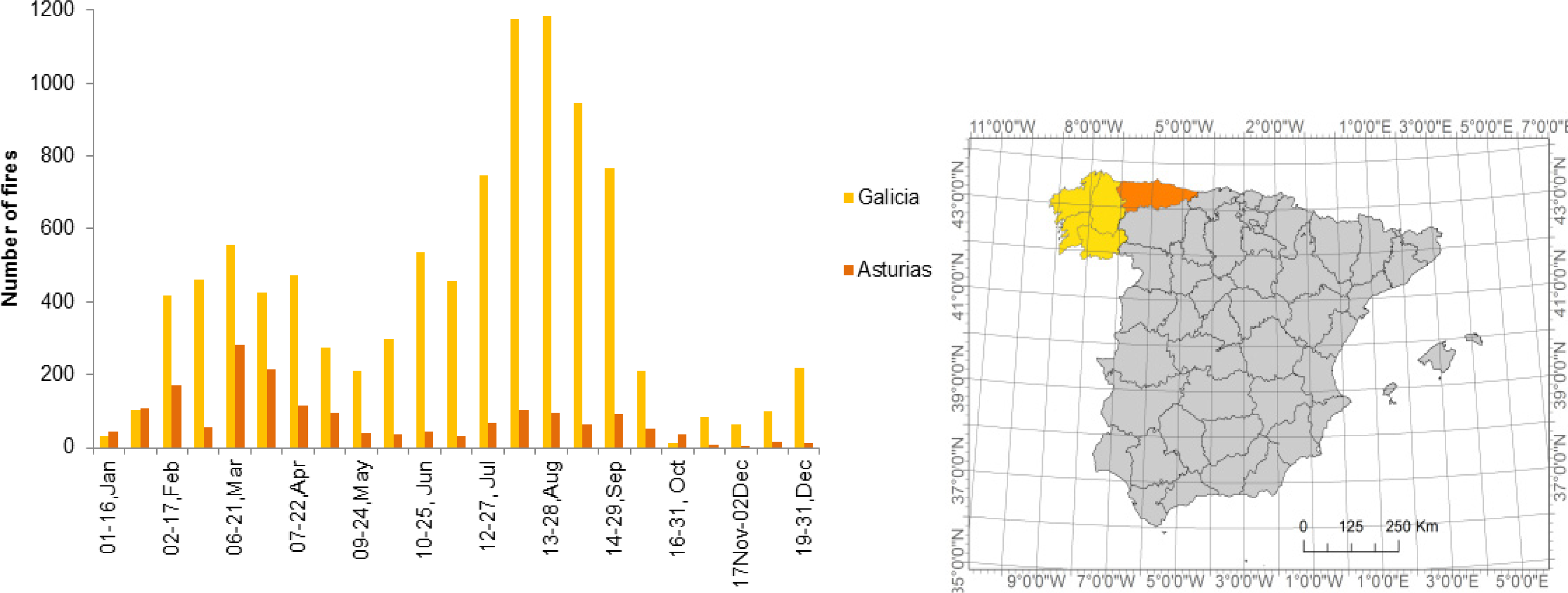
2. Study Area and Dataset
3. Methodology
3.1. MODIS Image Processing
3.2. Obtaining the Spectral Indices
3.3. Relationship between Fire Frequency and Changes in the Spectral Indices
3.4. Combining the Vegetation Index with Other VariaSDAbles
4. Results and Discussion
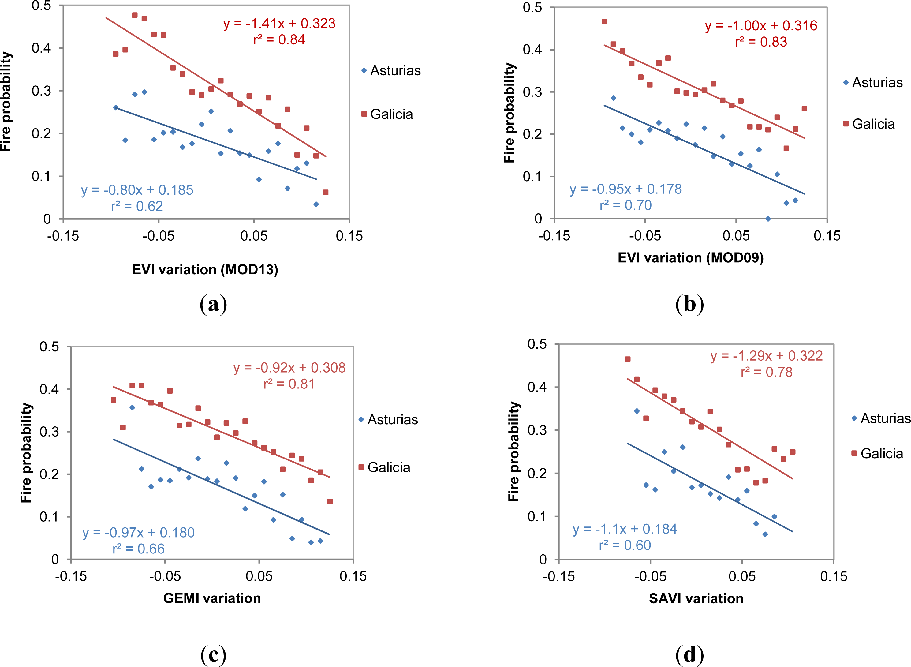
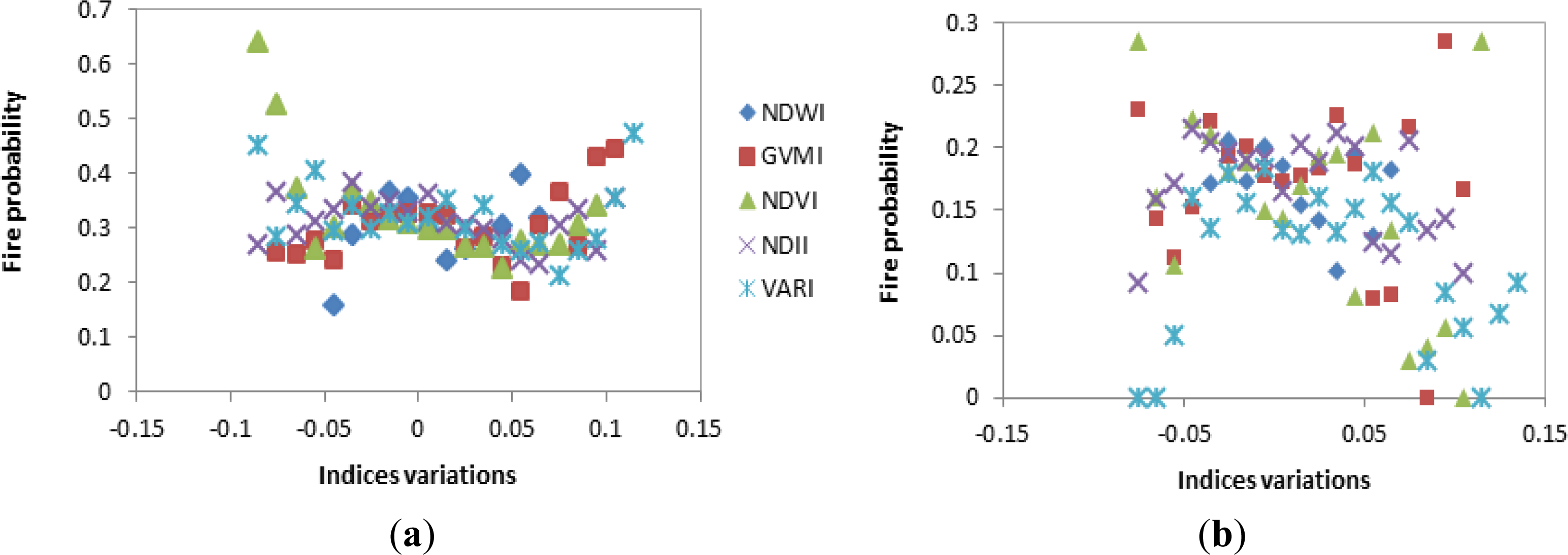
4.1. Vegetation Indices vs. Fire Frequency
4.2. Fire Danger Estimation by Using Logistic Regression
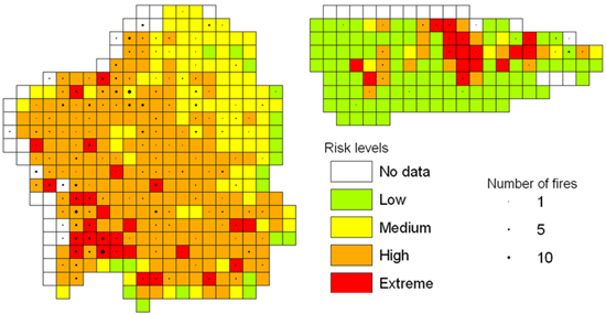
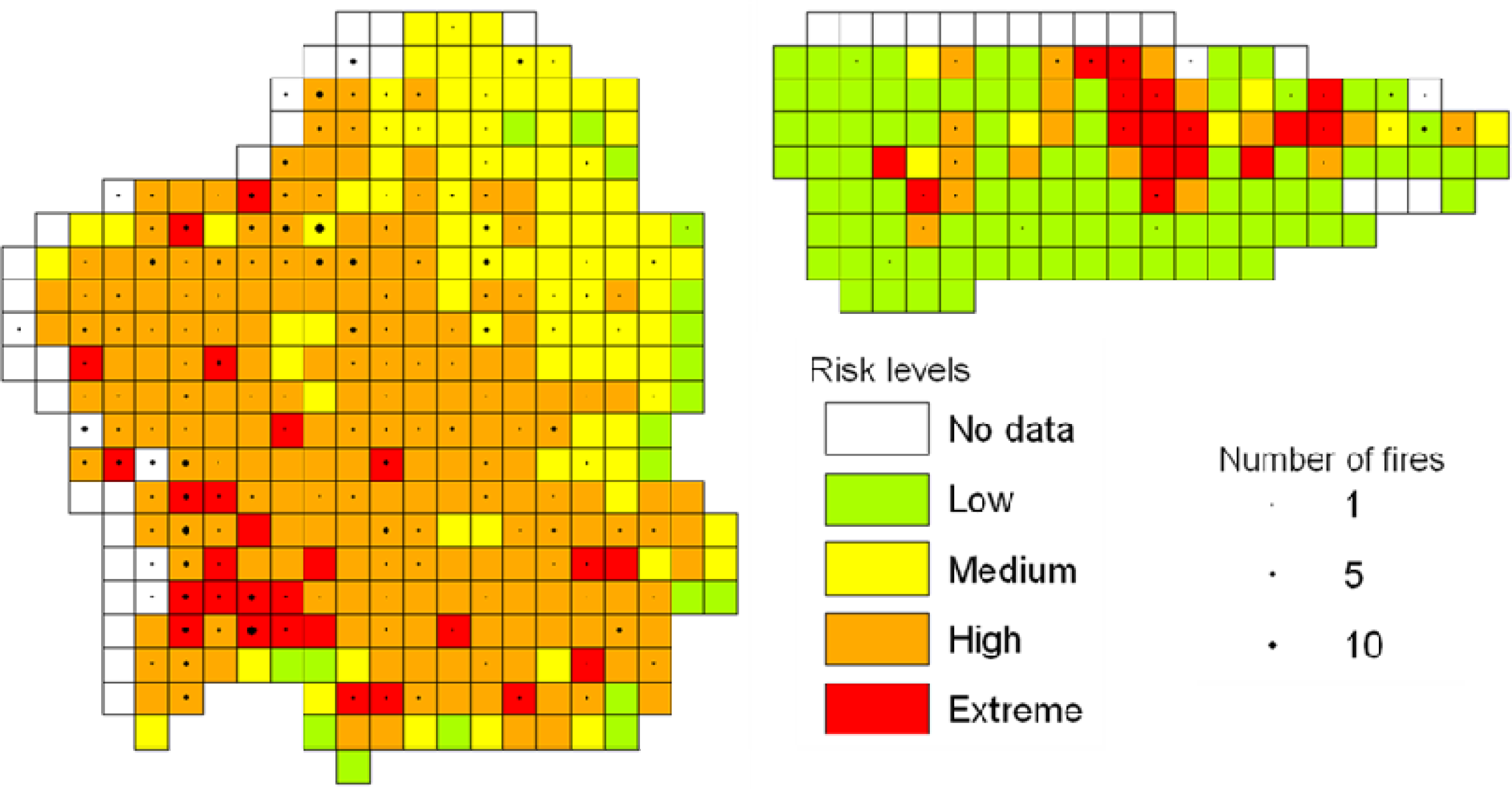
4.3. Fire Risk Levels
- Low risk: Probability < 21%
- Medium risk: 21% ≤ Probability < 32%
- High risk: 32% ≤ Probability < 52%
- Extreme risk: Probability ≥ 52%
5. Conclusions
Acknowledgments
Conflicts of Interest
References
- Martín, A.; Díaz-Raviña, M.; Carballas, T. Evolution of composition and content of soil carbohydrates following forest wildfires. Biol. Fertil. Soils 2009, 45, 511–520. [Google Scholar]
- Calvo, L.; Tárrega, R.; de Luis, E. The dynamics of Mediterranean shrubs species over 12 years following perturbations. Plant. Ecol 2002, 160, 25–42. [Google Scholar]
- Palacios-Orueta, A.; Chuvieco, E.; Parra, A.; Carmona-Moreno, C. Biomass burning emissions: A review of models using remote-sensing data. Environ. Monit. Assess 2005, 104, 189–209. [Google Scholar]
- Ministerio de Medio Ambiente. Los incendios forestales en España. Decenio 1996–2005. Available online: http://www.magrama.gob.es/es/biodiversidad/publicaciones/decenio_1996_2005_tcm7-19437.pdf (accessed on 23 December 2013).
- Xunta de Galicia Ley 3/2007, de 9 de abril, de prevención y defensa contra los incendios forestales de Galicia; Consellería de Medio Rural y del Mar, 2013. Available online: http://www.medioruralemar.xunta.es/fileadmin/arquivos/publicacions/2013/LeiDeIncendios/cast/Ley_03-07_de_prevenc_y_defensa_contra_los_incend__castellano_.pdf (accessed on 31 December 2013).
- Castro, F.; Tudela, A.; Sebastià, M. Modeling moisture content in shrubs to predict fire risk in Catalonia (Spain). Agric. For. Meteorol 2003, 116, 49–59. [Google Scholar]
- Alonso-Betanzos, A.; Fontenla-Romero, O.; Guijarro-Berdiñas, B.; Hernández-Pereira, E.; Inmaculada Paz Andrade, M.; Jiménez, E.; Luis Legido Soto, J.; Carballas, T. An intelligent system for forest fire risk prediction and fire fighting management in Galicia. Expert Syst. Appl 2003, 25, 545–554. [Google Scholar]
- Aguado, I.; Chuvieco, E.; Borén, R.; Nieto, H. Estimation of dead fuel moisture content from meteorological data in Mediterranean areas. Application in fire danger assessment. Int. J. Wildland Fire 2007, 16, 390–397. [Google Scholar]
- López, A.S.; San-Miguel-Ayanz, J.; Burgan, R.E. Integration of satellite sensor data, fuel type maps and meteorological observations for evaluation of forest fire risk at the pan-European scale. Int. J. Remote Sens 2002, 23, 2713–2719. [Google Scholar]
- Chuvieco, E.; Cocero, D.; Riaño, D.; Martin, P.; Martínez-Vega, J.; de la Riva, J.; Pérez, F. Combining NDVI and surface temperature for the estimation of live fuel moisture content in forest fire danger rating. For. Fire Prev. Assess 2004, 92, 322–331. [Google Scholar]
- Maki, M.; Ishiahra, M.; Tamura, M. Estimation of leaf water status to monitor the risk of forest fires by using remotely sensed data. Remote Sens. Environ 2004, 90, 441–450. [Google Scholar]
- Lozano, F.J.; Suárez-Seoane, S.; Kelly, M.; Luis, E. A multi-scale approach for modeling fire occurrence probability using satellite data and classification trees: A case study in a mountainous Mediterranean region. Remote Sens. Environ 2008, 112, 708–719. [Google Scholar]
- Schneider, P.; Roberts, D.A.; Kyriakidis, P.C. A VARI-based relative greenness from MODIS data for computing the Fire Potential Index. Remote Sens. Environ 2008, 112, 1151–1167. [Google Scholar]
- Lozano, F.J.; Suárez-Seoane, S.; de Luis, E. Assessment of several spectral indices derived from multi-temporal Landsat data for fire occurrence probability modelling. Remote Sens. Environ 2007, 107, 533–544. [Google Scholar]
- Leblon, B. Monitoring forest fire danger with remote sensing. Nat. Hazards 2005, 35, 343–359. [Google Scholar]
- Sow, M.; Mbow, C.; Hély, C.; Fensholt, R.; Sambou, B. Estimation of herbaceous fuel moisture content using vegetation indices and land surface temperature from MODIS data. Remote Sens 2013, 5, 2617–2638. [Google Scholar]
- Dennison, P.E.; Roberts, D.A.; Peterson, S.H.; Rechel, J. Use of Normalized Difference Water Index for monitoring live fuel moisture. Int. J. Remote Sens 2005, 26, 1035–1042. [Google Scholar]
- Stow, D.; Niphadkar, M.; Kaiser, J. MODIS-derived visible atmospherically resistant index for monitoring chaparral moisture content. Int. J. Remote Sens 2005, 26, 3867–3873. [Google Scholar]
- Wu, J.; Zhang, J.; Lü, A.; Zhou, L. An exploratory analysis of spectral indices to estimate vegetation water content using sensitivity function. Remote Sens. Lett 2011, 3, 161–169. [Google Scholar]
- Yebra, M.; Chuvieco, E.; Riaño, D. Estimation of live fuel moisture content from MODIS images for fire risk assessment. Agric. For. Meteorol 2008, 148, 523–536. [Google Scholar]
- Cheng, Y.-B.; Zarco-Tejada, P.J.; Riaño, D.; Rueda, C.A.; Ustin, S.L. Estimating vegetation water content with hyperspectral data for different canopy scenarios: Relationships between AVIRIS and MODIS indexes. Remote Sens. Environ 2006, 105, 354–366. [Google Scholar]
- Maselli, F.; Romanelli, S.; Bottai, L.; Zipoli, G. Use of NOAA-AVHRR NDVI images for the estimation of dynamic fire risk in Mediterranean areas. Remote Sens. Environ 2003, 86, 187–197. [Google Scholar]
- Verbesselt, J.; Jonsson, P.; Lhermitte, S.; van Aardt, J.; Coppin, P. Evaluating satellite and climate data-derived indices as fire risk indicators in savanna ecosystems. IEEE Trans. Geosci. Remote Sens 2006, 44, 1622–1632. [Google Scholar]
- Manzo-Delgado, L.; Sánchez-Colón, S.; Álvarez, R. Assessment of seasonal forest fire risk using NOAA-AVHRR: A case study in central Mexico. Int. J. Remote Sens 2009, 30, 4991–5013. [Google Scholar]
- Zhang, H.; Han, X.; Dai, S. Fire occurrence probability mapping of northeast China with binary logistic regression model. IEEE J. Sel. Top. Appl. Earth Obs. Remote. Sens 2013, 6, 121–127. [Google Scholar]
- Ministerio de Medio Ambiente Segundo Inventario Forestal Nacional. Escala 1:50,000 (1986–1995) 2007. Available online: http://www.magrama.gob.es/es/biodiversidad/servicios/banco-datos-naturaleza/informacion-disponible/ifn2.aspx (accessed on 31 December 2013).
- Instituto nacional de estadística. Anuario Estadístico de España 2008. Entorno físico y medio ambiente 2008. Available online: http://www.ine.es/inebmenu/mnu_medioambiente.htm (accessed on 31 December 2013).
- Martín-Vide, J.; Olcina, J. Climas y tiempos de España; Madrid Alianza Editorial: Madird, Spain, 2001. [Google Scholar]
- Huete, A.; Justice, C.; van Leeuwen, W. MODIS Vegetation Index (MOD13); Algorithm Theoretical Basis Document; 1999. Available online: http://modis.gsfc.nasa.gov/data/atbd/atbd_mod13.pdf (accessed 31 December 2013).
- Vermote, E.F.; Kotchenova, S.Y.; Ray, J.P. MODIS Surface Reflectance User’s Guide. MODIS Land Surface Reflectance Science Computing Facility; 2011. Available online: http://modis-sr.ltdri.org/products/MOD09_UserGuide_v1_3.pdf (accessed 31 December 2013).
- Bossard, M.; Feranec, J.; Otahel, J. CORINE Land Cover Technical Guide—Addendum 2000; Technical Report No 40; Copenhagen (EEA): Copenhagen, Denmark, 2000. [Google Scholar]
- Huete, A. A soil-adjusted vegetation index (SAVI). Remote Sens. Environ 1988, 25, 295–309. [Google Scholar]
- Rouse, J.W.; Haas, R.H.; Schell, J.A.; Deering, D.W. Monitoring Vegetation Systems in the Great Plains with ERTS. Proceedings of NASA Goddard Space Flight Center 3D ERTS-1 Symposium, Washington, DC, USA, 1974; 1, pp. 309–317.
- Hunt, E.R., Jr.; Rock, B.N. Detection of changes in leaf water content using near- and middle-infrared reflectances. Remote Sens. Environ 1989, 30, 43–54. [Google Scholar]
- Pinty, B.; Verstraete, M.M. GEMI: A non-linear index to monitor global vegetation from satellites. Vegetatio 1992, 101, 15–20. [Google Scholar]
- Gao, B. NDWI—A normalized difference water index for remote sensing of vegetation liquid water from space. Remote Sens. Environ 1996, 58, 257–266. [Google Scholar]
- Gitelson, A.A.; Kaufman, Y.J.; Stark, R.; Rundquist, D. Novel algorithms for remote estimation of vegetation fraction. Remote Sens. Environ 2002, 80, 76–87. [Google Scholar]
- Huete, A.; Didan, K.; Miura, T.; Rodriguez, E.; Gao, X.; Ferreira, L. Overview of the radiometric and biophysical performance of the MODIS vegetation indices. Remote Sens. Environ 2002, 83, 195–213. [Google Scholar]
- Ceccato, P.; Flasse, S.; Grégoire, J.-M. Designing a spectral index to estimate vegetation water content from remote sensing data: Part 2. Validation and applications. Remote Sens. Environ 2002, 82, 198–207. [Google Scholar]
- SPSS Inc. PASW STATISTICS 17.0 Command Syntax Reference; SPSS Inc: Chicago, IL, USA, 2009. [Google Scholar]
- Willmot, C.J. Some comments on the evaluation of model perfomance. Bull. Am. Meteorol. Soc 1982, 63, 1309–1313. [Google Scholar]


| Normalized Difference Vegetation Index | [33] | |
| Soil Adjusted Vegetation Index | , L=0.25 | [32] |
| Normalized Difference Infrared Index | [34] | |
| Global Environmental Monitoring Index | [35] | |
| Normalized Difference Water Index | [36] | |
| Visible Atmospheric Resistant Index | [37] | |
| Enhanced Vegetation Index | [38] | |
| Global Vegetation Moisture Index | [39] |
| Region | Index | A | B | R2 | Bias1 | RMSE2 | RMSES3 | RMSEU4 | MAD5 | MAPD6 |
|---|---|---|---|---|---|---|---|---|---|---|
| GALICIA | GEMI | 0.57 ± 0.09 | 0.13 ± 0.03 | 0.67 | −0.00017 | 0.05 | 0.04 | 0.04 | 0.04 | 12% |
| EVI | 0.62 ± 0.08 | 0.11 ± 0.03 | 0.73 | −0.007 | 0.05 | 0.03 | 0.03 | 0.04 | 11% | |
| SAVI | 0.59 ± 0.09 | 0.13 ± 0.03 | 0.71 | 0.006 | 0.05 | 0.04 | 0.04 | 0.04 | 13% | |
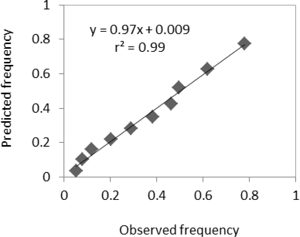
| EVI (MOD13) | 0.97 ± 0.10 | 0.01 ± 0.03 | 0.81 | 0.003 | 0.04 | 0.003 | 0.04 | 0.03 | 11% | |
| ASTURIAS | GEMI | 0.53 ± 0.12 | 0.08 ± 0.02 | 0.53 | −0.0016 | 0.05 | 0.03 | 0.04 | 0.03 | 19% |
| EVI | 0.65 ± 0.14 | 0.06 ± 0.03 | 0.54 | 0.004 | 0.04 | 0.02 | 0.04 | 0.03 | 19% | |
| SAVI | 0.47 ± 0.15 | 0.09 ± 0.03 | 0.41 | 0.003 | 0.05 | 0.04 | 0.04 | 0.03 | 21% | |
| EVI (MOD13) | 0.71 ± 0.12 | 0.06 ± 0.02 | 0.65 | 0.005 | 0.04 | 0.019 | 0.03 | 0.03 | 15% | |
| Variable | Coefficient | Standard Error | P (Wald) |
|---|---|---|---|
| EVI variation (MOD13) | −2.5 | 0.4 | < 0.001 |
| Period fire history | 31.6 | 0.6 | < 0.001 |
| Cell fire history | 282 | 7 | < 0.001 |
| Region (Asturias) | −2.66 | 0.07 | < 0.001 |
| Constant | −3.00 | 0.05 | < 0.001 |
| Observed | Predicted | |||||
|---|---|---|---|---|---|---|
| Training | Test | |||||
| No Fire | Fire | Concordance | No fire | Fire | Concordance | |
| No fire (0) | 10,412 | 4,389 | 70.3 | 10,545 | 4,407 | 70.5 |
| Fire (1) | 2,138 | 5,812 | 73.1 | 2,355 | 5,416 | 69.7 |
| Global concordance | 71.3 | 70.2 | ||||
© 2014 by the authors; licensee MDPI, Basel, Switzerland This article is an open access article distributed under the terms and conditions of the Creative Commons Attribution license ( http://creativecommons.org/licenses/by/3.0/).
Share and Cite
Bisquert, M.; Sánchez, J.M.; Caselles, V. Modeling Fire Danger in Galicia and Asturias (Spain) from MODIS Images. Remote Sens. 2014, 6, 540-554. https://doi.org/10.3390/rs6010540
Bisquert M, Sánchez JM, Caselles V. Modeling Fire Danger in Galicia and Asturias (Spain) from MODIS Images. Remote Sensing. 2014; 6(1):540-554. https://doi.org/10.3390/rs6010540
Chicago/Turabian StyleBisquert, Mar, Juan Manuel Sánchez, and Vicente Caselles. 2014. "Modeling Fire Danger in Galicia and Asturias (Spain) from MODIS Images" Remote Sensing 6, no. 1: 540-554. https://doi.org/10.3390/rs6010540