Article

High Spatial Resolution WorldView-2 Imagery for Mapping NDVI and Its Relationship to Temporal Urban Landscape Evapotranspiration Factors

1
SA Water Centre for Water Management and Reuse, University of South Australia, Adelaide, SA 5095, Australia
2
School of Natural and Built Environments, University of South Australia, Adelaide, SA 5095, Australia
3
Barbara Hardy Institute, University of South Australia, Adelaide, SA 5095, Australia
4
Sonoran Desert Research Station, Southwest Biological Science Center, US Geological Survey & University of Arizona, Tucson, AZ 85719, USA
*
Author to whom correspondence should be addressed.
Remote Sens. 2014, 6(1), 580-602; https://doi.org/10.3390/rs6010580
Submission received: 2 October 2013 / Revised: 25 November 2013 / Accepted: 18 December 2013 / Published: 6 January 2014

Abstract

:
Evapotranspiration estimation has benefitted from recent advances in remote sensing and GIS techniques particularly in agricultural applications rather than urban environments. This paper explores the relationship between urban vegetation evapotranspiration (ET) and vegetation indices derived from newly-developed high spatial resolution WorldView-2 imagery. The study site was Veale Gardens in Adelaide, Australia. Image processing was applied on five images captured from February 2012 to February 2013 using ERDAS Imagine. From 64 possible two band combinations of WorldView-2, the most reliable one (with the maximum median differences) was selected. Normalized Difference Vegetation Index (NDVI) values were derived for each category of landscape cover, namely trees, shrubs, turf grasses, impervious pavements, and water bodies. Urban landscape evapotranspiration rates for Veale Gardens were estimated through field monitoring using observational-based landscape coefficients. The relationships between remotely sensed NDVIs for the entire Veale Gardens and for individual NDVIs of different vegetation covers were compared with field measured urban landscape evapotranspiration rates. The water stress conditions experienced in January 2013 decreased the correlation between ET and NDVI with the highest relationship of ET-Landscape NDVI (Landscape Normalized Difference Vegetation Index) for shrubs (r2 = 0.66) and trees (r2 = 0.63). However, when the January data was excluded, there was a significant correlation between ET and NDVI. The highest correlation for ET-Landscape NDVI was found for the entire Veale Gardens regardless of vegetation type (r2 = 0.95, p > 0.05) and the lowest one was for turf (r2 = 0.88, p > 0.05). In support of the feasibility of ET estimation by WV2 over a longer period, an algorithm recently developed that estimates evapotranspiration rates based on the Enhanced Vegetation Index (EVI) from MODIS was employed. The results revealed a significant positive relationship between ETMODIS and ETWV2 (r2 = 0.9857, p > 0.05). This indicates that the relationship between NDVI using high resolution WorldView-2 imagery and ground-based validation approaches could provide an effective predictive tool for determining ET rates from unstressed mixed urban landscape plantings.

1. Introduction

In macro-scale water management, a precise prediction of water lost through evapotranspiration (ET) is always challenging, particularly when estimating ET from mixed vegetation types [1]. Some vegetation dynamics such as plant vigor, vegetation density and canopy cover can be quantified into biophysical parameters. Vegetation biophysical characteristics can be estimated from field measurements, aerial photography or satellite data visualization and interpretation. Although, the two traditional methods of ground measurement and aerial photography are regularly used, there have been significant advances in remote sensing (RS) that have increased the accuracy of vegetation analysis. The ground measurement methods are generally time-consuming and relatively expensive and often lead to a lack of coverage for large areas [2]. In contrast, satellite data cover large regions that do not need intensive ground measurement, although some field work helps to improve image interpretation. The spatial resolution of RS images has also been dramatically improved from hundreds of meters to the sub-meter level. In addition, the temporal resolution is now often near real time [3].
From the exploration of outer space in 1957 with the first man-made satellite up to 2013, there has been a rapid enhancement in the design and operation of satellites to observe the atmosphere and the Earth’s surface. In 1964, an Advanced Very High Resolution Radiometer (AVHRR) was included on the National Oceanic and Atmospheric Administration (NOAA) platforms to measure the red and near-infrared bands. In 1972, when Landsat1 was launched with its multi-spectral scanners, the first notion of possible correlation of vegetation biophysical characteristics to the red/infrared and other spectral ratios was established. This was termed a vegetation index (VI) and was gradually improved by enhanced spatial and spectral resolutions [4]. Various algorithms and models have since been introduced often employing GIS/RS applications to study the biophysical parameters of vegetation. Several mathematical combinations of different spectral bands and a variety of spectral reflectances have resulted in the development of different vegetation indices (VIs). Rouse et al. [5] proposed the NDVI to estimate plant vigor. Later, Huete [6] introduced a Soil Adjusted Vegetation Index (SAVI) and Kim et al. [7] proposed a Chlorophyll Absorption Ratio Index (CARI). In addition, Roujean and Breon [8] developed a Renormalized Difference Vegetation Index (RDVI). A modified CARI was introduced with potential for Leaf Area Index (LAI) estimation by Daughtry et al. [9]. A Triangular Vegetation Index (TVI) was introduced by Broge and Leblanc [10] and the Three-band Gradient Difference Vegetation Index (TGDVI) was developed by Tang et al. [11]. Although, numerous vegetation indices have been developed, most of these are based on the separation of vegetation from soil and water. In other words, RS-based VIs measure vegetation greenness optically to estimate such variables as vegetation cover, leaf chlorophyll content and leaf area. Application of VIs can vary spatially from leaves (e.g., LAI) to global scales (e.g., EVI from Nagler et al. [12,13]). This is because of the wide variety of satellites used, including MODIS, Landsat, ASTER, SPOT5, QuickBird, IKONOS, GeoEye, WorldView-1 and WorldView-2 with their different spatial, spectral, temporal, and radiometric resolutions. For instance, the most popular VI, the NDVI, relies on the principle concept of a relationship between absorption of visible light and resilient reflectance of near-infrared light to the chlorophyll in vegetation [13].
Nouri et al. [14,15] reviewed the relationship between agricultural and non-agricultural VIs and ET. They recommended VIs, and particularly NDVI, as a robust indicator to study vegetation characteristics and consequently ET rates. Statistical analysis and ground measurement has confirmed that a near linear relationship can be found between VIs and photosynthesis by vegetation canopy [16]. Long-term RS data analysis by Rossato et al. [17] showed that ET and NDVI have a near-linear relationship. A linear relationship between NDVI and basal crop coefficient for irrigated agricultural fields was also reported by Duchemin et al. [18].
The research presented in this paper investigates the possible relationship between remotely-sensed NDVI and observational-based field estimations of urban landscape ET. For this study, WorldView-2 satellite images were processed. Three landscape coefficients were estimated through field monitoring and in-situ weather data acquisition, these being Water Use Classifications of Landscape Species (WUCOLS), Plant Water Use Factor (PF), and Best Practice Code of Irrigated Public Open Space (IPOS).

2. Methods and Materials
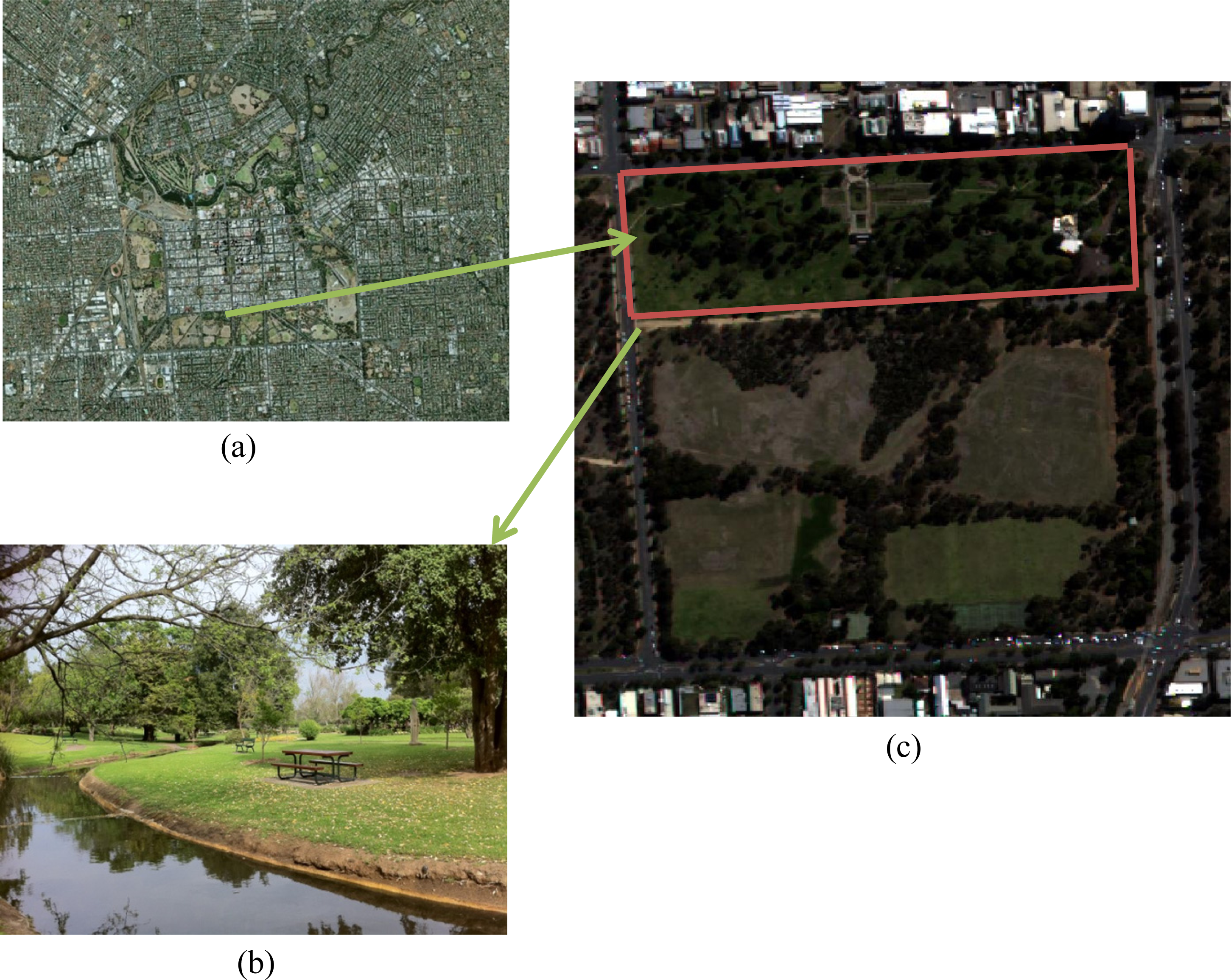
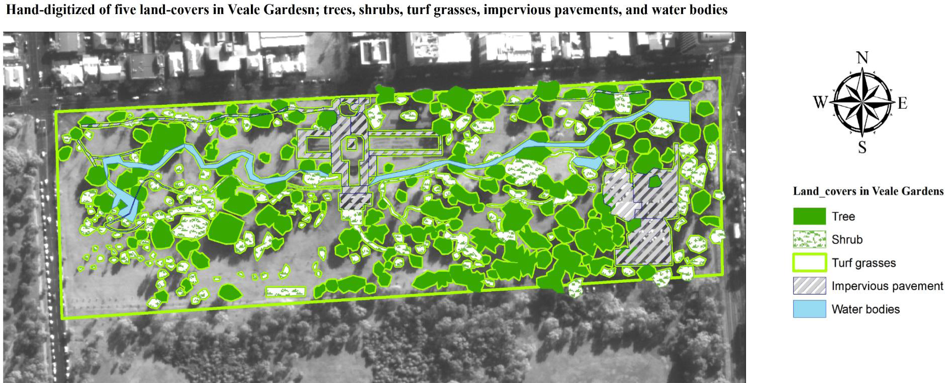
2.1. Study Area

The study area shown in Figure 1 consists of a 9.6 hectare urban park named Veale Gardens which is located within the Adelaide Parklands in the city of Adelaide in South Australia. Veale Gardens is located between latitudes of 34.9357 and 34.9376S and longitudes of 138.5945 and 138.6002E. The area is semi-arid with an average annual rainfall of 549 mm and with a mean maximum temperature of 42.8 °C in January and fairly cold winters (June–August), with a mean minimum temperature of 2.2 °C in June. The park contains more than 60 different species, size and type of landscape trees and shrubs with an additional broad coverage of Kikuyu turf grass, which is irrigated using a sprinkler system.

2.2. Satellite Data

NDVI images were prepared from high resolution WorldView-2 images covering Veale Gardens. WorldView-2 (WV2), which is a high spatial and spectral resolution satellite, provides eight spectral bands in the visible to near-infrared range and covers 975,000 km2 per day. It has an average revisit time of 1.1 days with a swath width of 16.4 km at nadir. The range of four standard bands (red, green, blue, and NIR1) and four new bands (coastal blue, yellow, red-edge, and NIR2) (Table 1) enhances spatial and spectral analysis, mapping and monitoring of large areas with great details, and deeper vegetation analyses [2].
Satellite images were obtained from DigitalGlobe at approximately quarter year intervals to track vegetation changes from February 2012 to February 2013 (Table 2).

2.2.1. Vegetation Indices

Several research studies have successfully developed ET prediction models using VIs for different vegetation covers [19] including shrub lands [20,21], riparian sites [2225], and over regional scales with a variety of land covers/land uses of grasslands to forests [26,27]. NDVI, the most widely used VI, quantifies the vegetation’s photosynthetic response to red radiation absorption and near infrared reflectance [2833]. For most satellites, NDVI is computed from Equation 1:
NDVI = ( ρ NIR ρ red ) / ( ρ NIR + ρ red )
where ρNIR is the reflectance of the near-infrared wavelength band and ρred is the reflectance of the red wavelength band.
A number of normalized difference indices have been created and employed from WV2 images. For instance, Xiaocheng et al. [34] employed four different normalized difference indices, namely the Normalized Difference Bare Soil Index (NDBSI) created from blue and coastal blue, Normalized Difference Water Index (NDWI) from green and NIR2, NDVI from red and NIR1, and Forest and Crop Index (FCI) from red-edge and NIR1. Wolf [35] worked with four indices, namely NDWI, NDVI, Normalized Difference Soil Index (NDSI) from green and yellow, and Non-homogeneous Feature Difference (NHFD) from red-edge and coastal bands. De Benedetto et al. [36] calculated NDVI from red and NIR1 bands and Normalized Difference Red Edge (NDRE) from NIR and red-edge bands. Eckert [37] referred to NDVI1 using NIR1 and red and NDVI2 using NIR2 and red.
From the 64 possible two band combinations of eight WV2 spectral bands to compute vegetation ratios [38,39], the five most reliable combinations that were recommended by Pu and Landry [2] are shown in Table 3.
Pu and Landry [2] computed the five NDVI images (NDVIs) shown in Table 3 and a further five atmospheric corrected NDVIs (aNDVIs). A similar analysis procedure was used in this study on Veale Gardens for NDVI mapping, as shown in Figure 2. First, every image was checked for orthorectification. The orthorectification process resulted in very little accuracy change in the imagery because of the flatness of the terrain in the study area. Then, the area of interest was delineated. Atmospheric correction was required due to differences in sun positions for the time of the day and day of the year, changes in solar elevation angle from summer to winter and terrain effects that may cause differential solar illumination. The widely-used ATCOR model software based on MODTRAN calculations was employed for atmospheric correction [4042].

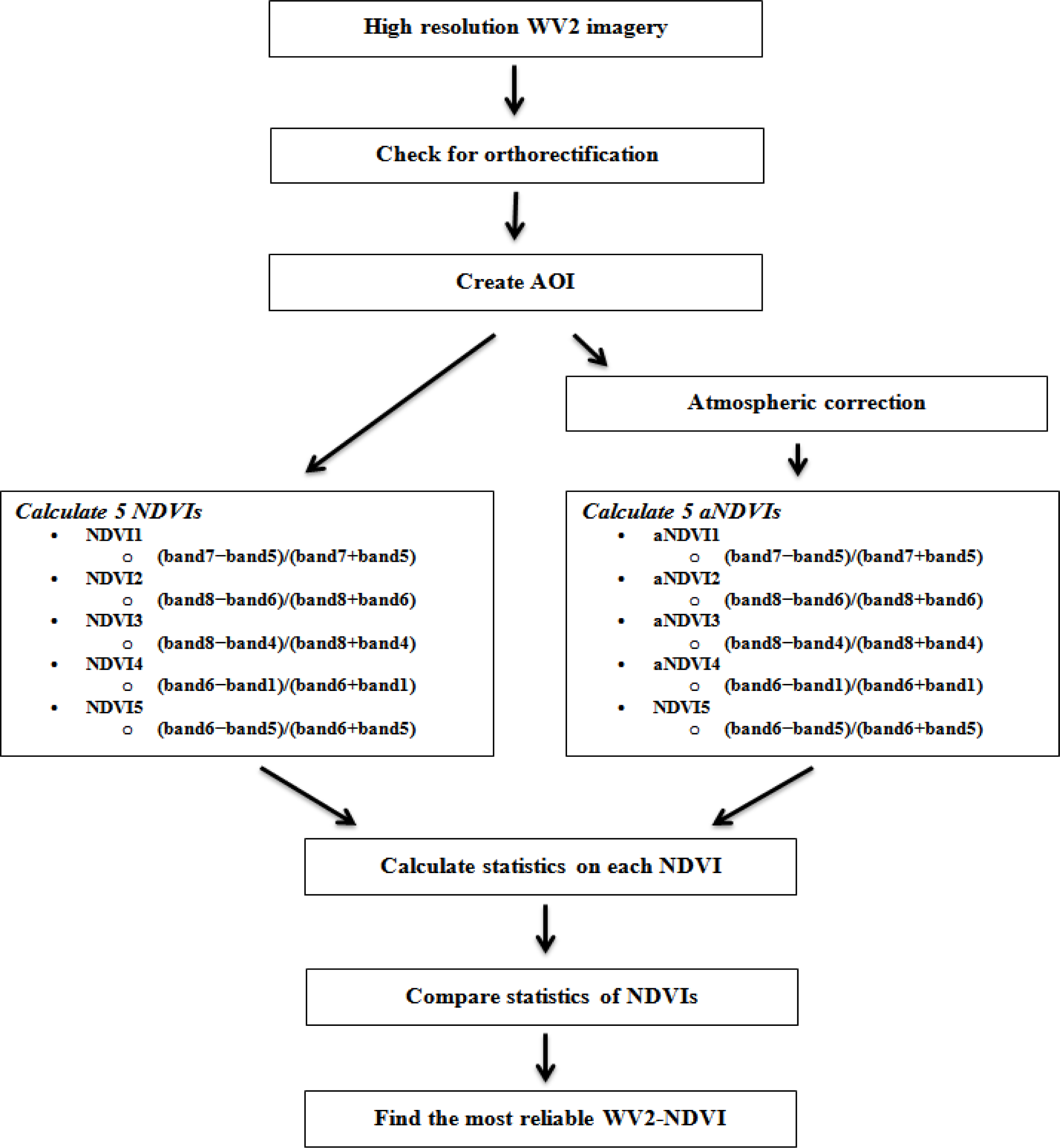
2.2.2. Satellite Imagery Data Processing

A data set of five WV2 images taken on 18 March 2012, 29 June 2012, 17 August 2012, 9 November 2012 and 16 January 2013 were compiled (Figure 3).
These images covered 25 km2 of the Adelaide area. Both panchromatic and multispectral images were orthorectified by DigitalGlobe (pixels at 0.5 and 2 m, respectively). ERDAS IMAGINE 2013 was employed to confine a rectangular area of interest (AOI) (Figure 3). As a prerequisite for atmospheric correction, each image was geo-referenced. ATCOR 2 was adopted as an add-on module to ERDAS IMAGINE to allow two dimensional atmospheric corrections [43]. An NDVI model using bands 7 and 5 was built and generated to create an NDVI image of the AOI. This NDVI image was clipped to the Veale Gardens borders and zonal statistics were applied to calculate the NDVI of the entire Veale Gardens. Simultaneously, panchromatic imagery was used as a base map from which to digitize different surface cover types in Veale Gardens. These types included trees, shrubs, turf grasses, impervious pavements and water bodies. The generated NDVI image of the AOI was overlayed to digitized landcover subsets of Veale Gardens to calculate the zonal statistics of the NDVI for each cover type (Figure 4).

2.3. Field Data

The ET rates of mixed urban landscape plants were determined using three different observational-based approaches [44]. Adjustment factors were applied as a fraction to the reference ET to estimate the plant water requirements in order to achieve the optimum plant health and acceptable aesthetic conditions. The relationship between adjustment factor and ET rate is expressed by Equation (2):
ET L = K L × ET ref
where ETL is the ET of urban landscape plants (mm/day), KL is an adjustment factor (landscape plant coefficient), and ETref is the reference ET in mm/day [4548].
The three field-based adjustment factor approaches used in this study were: (i) Water Use Classifications of Landscape Species (WUCOLS); (ii) Plant Water Use Factor (PF); and (iii) Best Practice Code of Irrigated Public Open Space (IPOS).
In WUCOLS, which is the first of the field-based methods, KL is determined by multiplying species, density and microclimate factors to determine the overall landscape coefficient [4749].
The species factor varies for different plant types depending on the water requirements of the species established in the landscape. A list of 2000 species in six regions of California was presented by Costello and Jones [47,48] and they classified plants into four classes of water demand, namely very low, low, moderate and high. The species factor for these classes ranges from 0.1 to 0.9. In Veale Gardens, a list of the most common plant species was compiled and the recommended principles for assigning a species factor were followed. In addition, a team of professional horticulturists working in Veale Gardens assessed the list of plants in Veale Gardens in terms of water requirements and drought tolerance.
The density factor takes into account differences in canopy cover and vegetation tiers that result in different water losses. The factor varies from 0.5 for immature and sparse plantings to 1.3 for a broad coverage of ground cover with dense shrubs and trees. Based on WUCOLS principles, for mixed vegetation types when one vegetation type is predominant while another one occurs occasionally in the planting, the density of canopy cover is within the average category [48] which describes Veale Gardens.
The microclimate factor is used to modify the species and density factors to take account of urban features such as building and paving, which influence both water losses and the water demand of urban vegetation. The microclimate factor ranges from 0.5 to 1.4.
In addition to WUCOLS, a second field-based adjustment method was considered in this study, namely the Plant Water Use Factor (PF), which defines a landscape coefficient for the minimum irrigation needs to maintain acceptable function aesthetics aspects [50]. Pittenger et al. [51] produced a list of landscape plants and their PF factors.
A third field adjustment method, IPOS, was developed using a best practice guideline for the management of turf to a ‘fit for purpose’ standard [52]. In the IPOS method, the landscape factor is the product of a plant factor and plant stress factor that varies from 0.4 for passive recreational turf to 1.0 for elite sport turf. This is the method that formed the basis of the original irrigation design for Veale Gardens.
Reference evapotranspiration data was obtained from quality controlled Bureau of Meteorology (BOM) data for the nearest station, which is at Kent Town (KT), located on the east side of the city, 2.92 km from Veale Gardens. Kent Town (Station 023090) data were downloaded from the BOM website ( http://www.bom.gov.au/climate/data/).
These produced three landscape coefficients (KL) which when multiplied by the reference ET produced three field estimated ET rates (ETWUCOLS, ETPF, and ETIPOS). The detailed field testing procedures for each method have been reported in Nouri et al. [44,53]. The ET field data from these three methods were used to validate the remotely-sensed ET estimation methods described in this paper.

2.4. Correlating ET and NDVI

Spatial analysis was employed in order to evaluate the relationship between ET of urban landscape plants and remotely sensed NDVI. Reflectance values for each landcover subset in Veale Gardens were extracted from the generated NDVI image using overlay analysis in ArcGIS. Then, linear regression was used to analyze the relationship between NDVIs and ETWUCOLS, ETPF, and ETIPOS. The coefficients of determination (r2) were then plotted to show the variation in the strength of the relationship between NDVI and ET. Selection of the best NDVIs and ETs for further analysis was based on their r2 values.

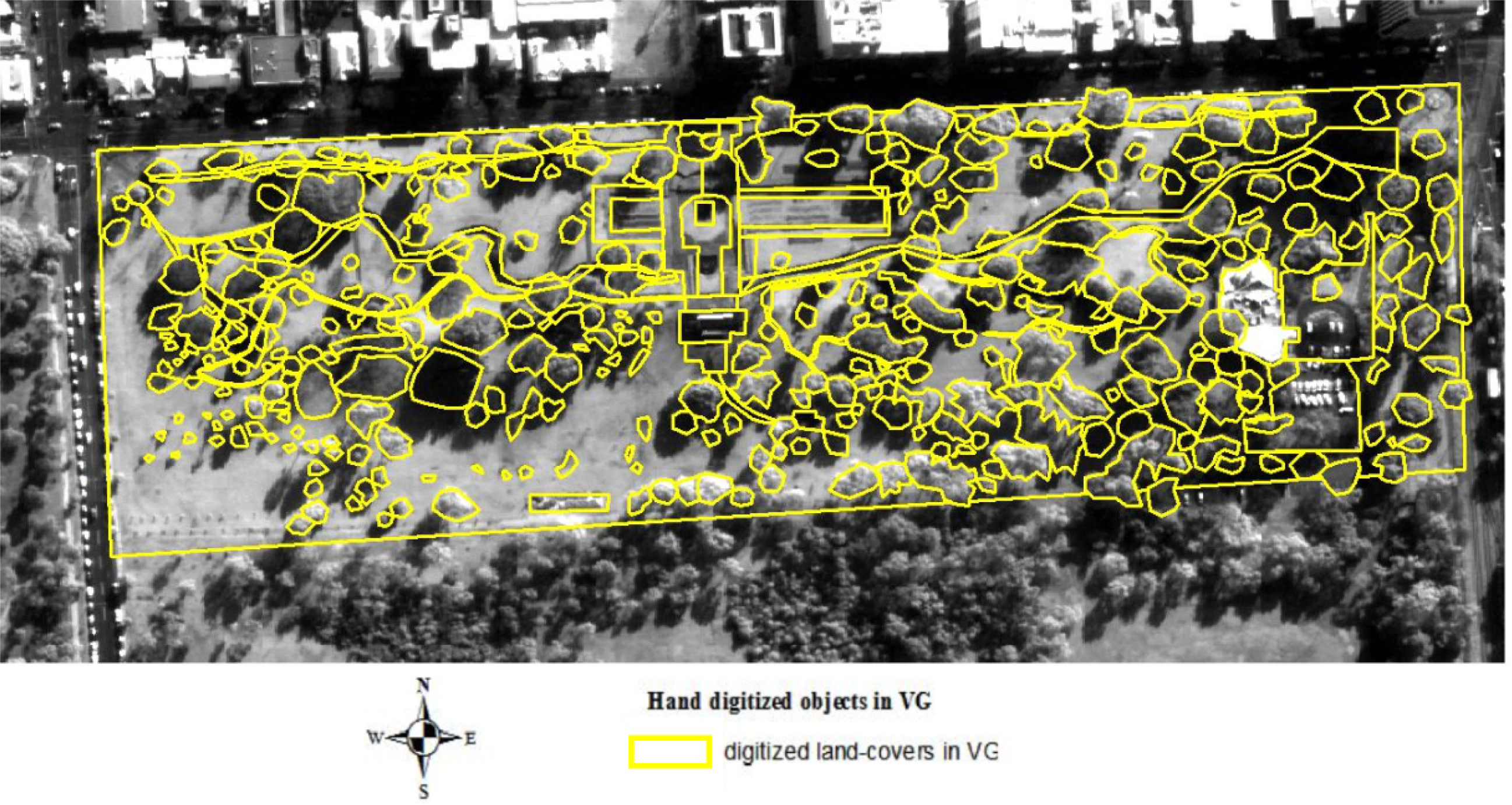
2.5. Independent Remotely-Sensed ET Estimation in Veale Gardens

Although the motivation of this research was to assess the capability and feasibility of remotely sensed VIs for predicting evapotranspiration of mixed urban vegetation, the authors additionally have investigated an independent measure of ET using satellite derived data. The authors employed a recently published remotely sensed algorithm by Nagler et al. [12] using Enhanced Vegetation Index (EVI) from MODIS for ET estimation in Veale Gardens mixed vegetation area. EVI (Equation (3)) was developed as an index to compensate for canopy background noises and topographic variations [6,22].
EVI = 2.5 × ( NIR Red ) / ( 1 + NIR + ( 6 × Red 7.5 × Blue ) )
where the coefficient “1” accounts for canopy background scattering and the blue and red coefficients, 6 and 7.5, minimize residual aerosol variations.

3. Results

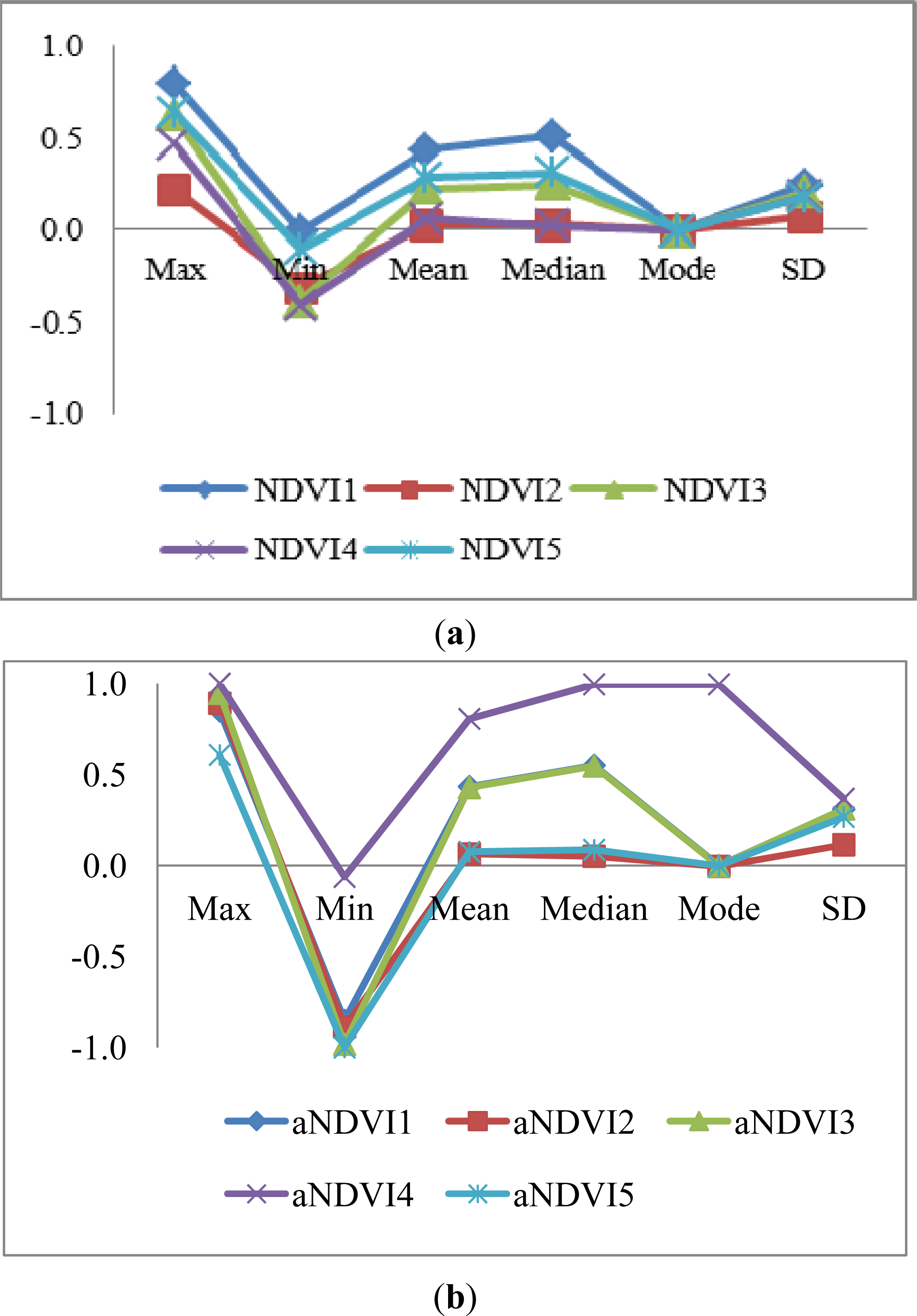
3.1. Selecting the Most Reliable NDVI from WV2 Images

Different combinations of spectral bands were employed to model different NDVIs, as shown in Figure 2. A similar process was applied on the atmospheric corrected images to develop aNDVIs. The statistical analysis of five NDVIs and five aNDVIs revealed a greater range in most statistical properties for aNDVIs than for NDVIs (Figure 5).
Considering the importance of temporal changes in NDVI and the significant differences in aNDVIs, the authors selected aNDVI1 as the most reliable NDVI for further analysis. The significant difference in median of NDVI1 and aNDVI1 compared to similar pairs resulted in the selection of aNDVI1. Because of the application to urban landscape plants, aNDVI1 will henceforth be referred to as Landscape NDVI.

3.2. Temporal Variation of Mean NDVI for Veale Gardens

The geospatial border of Veale Gardens was hand digitized using panchromatic imagery and field observations (Figure 6). All the steps mentioned in Figure 4 were followed to develop Landscape NDVI images of AOI in ERDAS Imagine and then clipped to the Veale Gardens border in ArcGIS. Zonal statistics were applied to calculate the statistical parameters of Landscape NDVI for the entire Veale Gardens for each image. The mean and standard deviation of Landscape NDVIs of all five images are shown in Table 4.

3.3. Temporal Variation of Landscape NDVIs for each Vegetation Type in Veale Gardens

The geospatial boundaries of different objects in Veale Gardens were hand digitized using panchromatic imagery, aerial imagery and field observations (Figure 6).
If the center of a pixel fell within a defined category, it was taken to belong to that category. From the hand-digitized objects map, five land cover classes were defined for analysis. These classes corresponded to trees, shrubs, turf grasses, impervious pavements and water bodies. However, NDVI analysis was limited to the three vegetation cover types of trees, shrubs and turf grasses. The land cover classes are shown in Figure 7 as trees in green, shrubs in textured-green, impervious pavements in textured-grey, water bodies in blue and the remaining uncolored areas are turf grasses.
The Landscape NDVI values for the five landcover types in all five WV2 images were calculated using ERDAS IMAGINE and overlayed by landcover maps in ArcGIS as described in Figure 4. The zonal statistics of Landscape NDVI for each vegetation cover type within the study period are listed in Table 5.

3.4. Observation-Based Landscape Evapotranspiration

In order to assign a landscape coefficient, KL, for Veale Gardens, three observational-based approaches were employed. Due to the heterogeneity of vegetation and availability of mixed plantings, a species factor of 0.53 was allocated to Veale Gardens. This was based on field observations of different landscape species and the advice of a water expert panel, who advised that the majority of the species were in the category of plants with a moderate water requirement. Considering the fact that most of the park is covered by Kikuyu turf grasses with sparse trees and shrubs, a density factor of 1 was assigned. A microclimate factor of 1.05 was selected for the whole park considering the minor influence of surrounding urban features including parking lots, streets and buildings in the park. Hence, an overall WUCOLS landscape coefficient of KL = 0.56 was calculated for Veale Gardens.
The PF approach uses research-based field data for estimation of landscape plants’ water requirements. A PF landscape factor of 0.5 was assigned for Veale Gardens corresponding to PF principles that have been comprehensively described by Nouri et al. [44]. The plant landscape factors, PF, for certain landscape plants in specific regions were reported by Pittenger et al. [51]. For plants where PF is unknown, an initial value of 0.5 was recommended.
The IPOS method mainly focuses on turf grasses within a mixture of trees and shrubs in an urban landscape planting. The IPOS adjustment factor is quantified by combining crop coefficients with crop stress factors [52]. In Veale Gardens, a crop factor of 0.6 was assigned to Kikuyu turf grasses and a value of 0.4 was assigned to the crop stress factor resulting in an overall IPOS landscape factor of KL = 0.24 for Veale Gardens.
For the period February 2012 to February 2013, monthly ET values were estimated by multiplying reference evapotranspiration data from a quality controlled Bureau of Meteorology (BOM) station at Kent Town by the KL values for WUCOLS, PF and IPOS (Figure 8). The differences between ETIPOS and ETWUCOLS and WTPF can be explained by the IPOS key principles. This method mainly focuses on turf grasses within a mix of trees and shrubs in an urban landscape planting [52]. As the results show, turf grasses often have low NDVIs and so prediction of vegetation water requirement based on turf grasses may often lead to insufficient irrigation volumes. The reason for including IPOS in these results is that IPOS was used as the basis for the irrigation design in Veale Gardens.

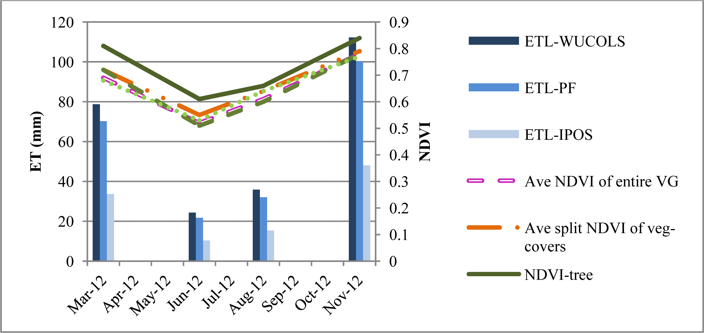
3.5. Temporal Variation of ETL, Mean Landscape NDVI and Landscape NDVIs for Different Vegetation Types

The mean Landscape NDVI for the entire Veale Gardens was calculated by statistical analysis of the Landscape NDVI image limited to the extent of the Veale Gardens borders. The mean Landscape NDVI was calculated as a product of each vegetation type’s Landscape NDVI and its area divided by the total area of Veale Gardens that is covered by trees, shrubs and turf grasses. The corresponding landscape ET is shown in Figure 8. The temporal variations of ET (WUCOLS, PF and IPOS), mean entire Veale Gardens Landscape NDVI (including water bodies and impervious pavements), mean total vegetation cover Landscape NDVI (includes the three vegetation types but not water bodies or impervious pavements), and Landscape NDVI for each individual vegetation cover (trees, shrubs and turf grasses) are plotted in Figure 9. The highest Landscape NDVIs are in November and the lowest values are in June. Of the three vegetation covers, trees had the highest Landscape NDVI values in the whole year and turf grasses had the lowest Landscape NDVI values except in winter time.

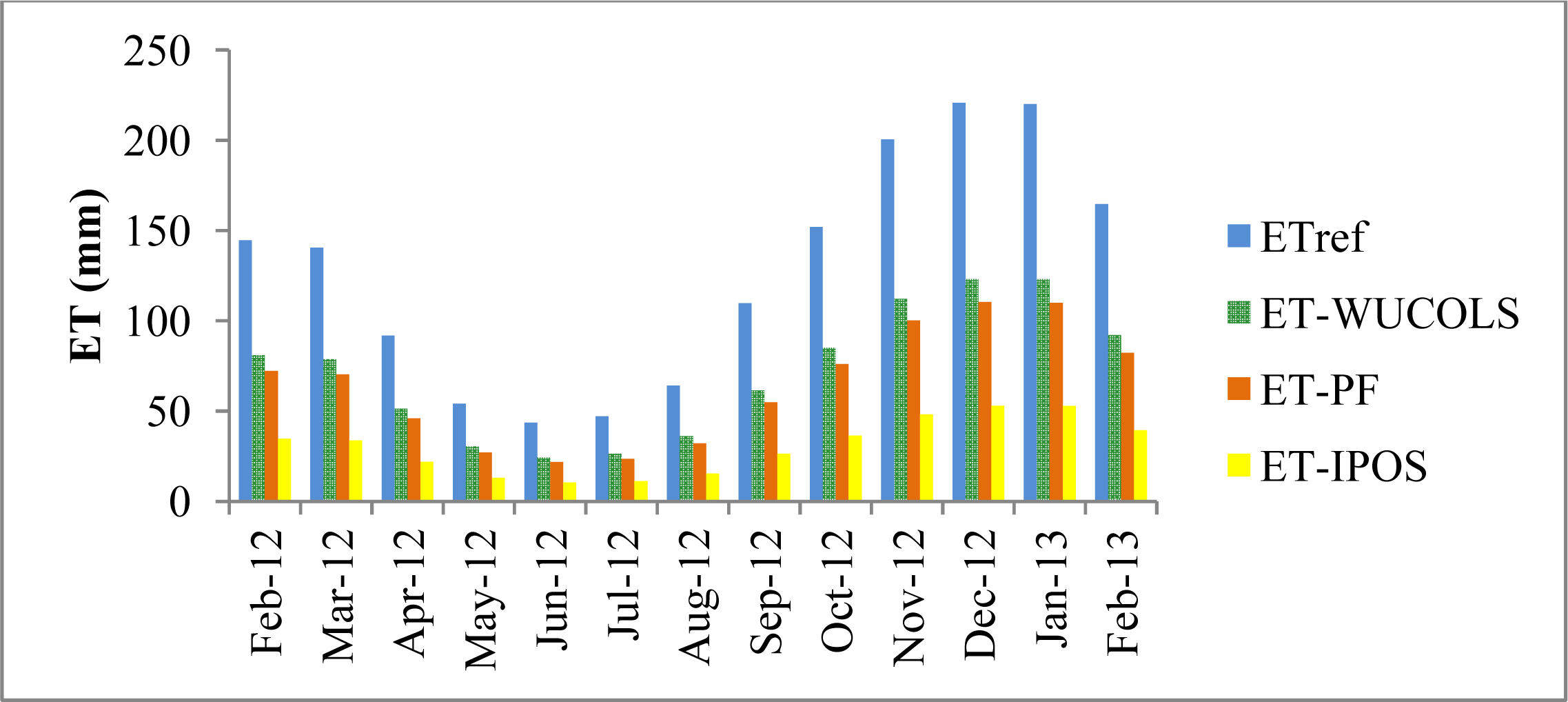
3.6. Independent Remotely-Sensed ET Estimation Using MODIS-EVI

The results of using remotely-sensed ET estimation using MODIS-EVI and local meteorological station potential ET (collected from the Australian Bureau of Meteorology, www.bom.gov.au) to estimate ET rates in Veale Gardens during 2000–2013 are presented in Figure 10.
The relationship between ET estimation of the MODISEVI algorithm and ground-based ET estimation using the WUCOLS approach was investigated (Figure 10). The results show a significant positive relationship between ETMODIS and ETWUCOLS (r2 = 0.9902).

4. Discussions

Landscape NDVI values (Figure 9) display the expected annual vegetation greenness pattern (as represented by NDVI). This shows the greenness starting as relatively high in late summer (March) and then reducing to a minimum in winter (June), before starting to green up in spring (August) and peaking again in November. Low winter temperatures in Adelaide lead to winter dormancy in most species of shrubs and kikuyu turf grasses. This resulted in the lowest Landscape NDVI of the year. Low rainfall and very high ET rates in January are two factors that may have caused a drop in the Landscape NDVI rate compared to the highest Landscape NDVI values in November.
There is not a significant difference between the mean Landscape NDVI for the entire Veale Gardens (regardless of cover type) and the mean Landscape NDVI of three combined vegetation covers (trees, shrubs, and turf grasses). The lack of significance might be related to the low coverage of water bodies and impervious pavements in Veale Gardens. The authors recommend a similar approach for different study areas to investigate potential differences between NDVI derived from different vegetation covers and average NDVI for an entire urban park. However, the mean Landscape NDVIs for the three vegetation covers were higher than the mean Landscape NDVI for the entire Veale Gardens. The largest difference in the NDVI average values was only 5.7% between the three vegetation covers and the entire park values.
The results of a previous study by the authors confirmed that the acceptable aesthetic and healthiness levels of vegetation of Veale Gardens was achieved by the WUCOLS method, which produced the best estimation of urban vegetation water requirements [44]. In this study, the possible relationship between ETWUCOLS and Landscape NDVI has been examined. A linear regression analysis of Landscape NDVI values versus ETWUCOLS shows that the highest predictable relationship is between landscape ET rates and Landscape NDVI of shrubs and trees (r2 = 0.66, p > 0.05; r2 = 0.63, p > 0.05), respectively compared to the lowest predictable relationship with turf and Landscape NDVI (r2 = 0.34, p > 0.05) (Figure 11).
Data analysis shows a consistent trend between Landscape NDVIs and ET rates with the exception of January 2013. The meteorological records for Kent Town show that the January 2013 rainfall was only 61.1% of the average 30-year rainfall history for this month. This led to a drier vegetation cover which in turn negatively influenced the greenness of the turf grasses, as can be seen in Figure 11.
The January 2013 results were considered as outliers because this image had 22% cloud cover compared to the other images, which all had 0% cloud cover. Therefore the January 2013 results were excluded from the analysis. Figure 12 shows a strong relationship between Landscape NDVIs and ETWUCOLS during 2012. The highest predictable relationship was found between ET and Landscape NDVI for the entire Veale Gardens regardless of vegetation type (r2 = 0.95, p > 0.05) and the lowest was between ET and turf-Landscape NDVI (r2 = 0.88, p > 0.05), although this was still quite high.
These results show that the ET estimations using WV2-NDVI model were a good indicator of the ET of urban landscape plants for Veale Gardens when January 2013 data was excluded (Figure 13). The strong significant positive correlation between ETWV2 and ETWUCOLS (r2 = 0.96, p > 0.05) demonstrates well the feasibility and practicality of a remotely-sensed ET estimation approach in Veale Gardens. This finding is in line with several studies that have found a strong and reliable relationship between aerial-satellite-based Landscape NDVI measurements and ground-based ET measurements [17,5359]. A significant decrease in rainfall in January 2013 imposed stress conditions to the vegetation in Veale Gardens. This finding is in line with Nagler et al. [23] and Glenn et al. [57] who found that remotely sensed ET using a VI approach is a good estimator only in unstressed conditions. Glenn et al. [57] recommended multiple ET measurements over a site to enhance the accuracy and they also suggested considering the salinity and hydraulic gradients that greatly affect ET measurements.
Also, the relationship between remotely-sensed ET estimation using MODIS-EVI and BOM data and remotely-sensed ET estimation using WV2-NDVI was investigated (Figure 14). The results showed a significant positive relationship between ETMODIS and ETWV2 (r2=0.9857, p>0.05). A t-test analysis showed only a 3.3% difference between means of ETMODIS and ETWV2, which supports the legitimacy of comparison (using a paired, two-tailed, t-test with p = 0.78).

5. Conclusion

The objective of the research was to estimate ET of urban vegetation at a local scale using high resolution satellite data, which is not widely published in the remote sensing literature. This has been mainly due to the newly available WV2 imagery which can address previous limitation issues such as not only the size of the regions of interest for most urban parks and landscape features but also the permission and accessibility to these areas.
Despite these challenges associated with scaling in-situ ETL measurements for mixed urban landscape plants, the authors assessed the correlation between ground-based ET and ET derived from multi-seasonal WV2 imagery using four scenes over a city park area of mixed vegetation in Adelaide, South Australia, during the year 2012. Remotely sensed ET using NDVI (ETWV2) showed the highest correlation to ETWUCOLS. This significant positive correlation (r2 = 0.88–0.95 for the four image acquisitions) between ETWUCOLS and ETWV2 demonstrated the performance and validity of a remotely-sensed ET estimation approach using high resolution images from WV2. The results from ET estimation using coarse resolution MODIS imagery strongly support the capability and feasibility of predicting ET rates for mixed urban vegetation. Thus, this study has successfully developed a model describing the relationship between ET from urban landscape plants and remotely-sensed VI models in Veale Gardens. Moreover, the use of MODIS over Veale Gardens shows variability in water demand since 2000 demonstrating that this method can be used for monitoring purposes.
Considering the fact that all Australian states, including South Australia, have weather station networks, daily reference ET measurements for important urban green spaces and agricultural sites are also readily available. By accounting for field conditions, this remotely sensed method can provide practical, simple, quick and low-cost urban vegetation ET estimates compared with more expensive field-based approaches. This method of urban landscape water requirement estimation is highly beneficial and reliable as it is not dependent on extensive field data collection programs or on expensive airborne photographs.

Acknowledgments

This study was funded by the SA Water Corporation through Research Grant SW100201. The researchers are also grateful to staff at SA Water and particularly to Karen Rouse and Greg Ingleton. We also appreciate the support of Adelaide City Council and particularly Kent Williams, Adam Gunn and all the horticulturists and gardeners working in Veale Gardens. The researchers also acknowledge the support of the Goyder Institute for Water Research. The authors thank Edward Glenn from University of Arizona for his review of the manuscript. We also thank the Australian Bureau of Meteorology for providing meteorological data. Finally, we are very grateful for the assistance of Paul Sutton, David Bruce, Ali Hassanli, Sattar Chavoshi, Fatemeh Kazemi and technical officers in the School of Natural and Built Environments at the University of South Australia. We also appreciate the advice of Jorg Hacker of Flinders University. Any use of trade, product, or firm names is for descriptive purposes only and does not imply endorsement by the US Government.

Conflicts of Interest

The authors declare no conflict of interest.

References

  1. Sumantra, C. A Modified Crop Coefficient Approach for Estimating Regional Evapotranspiration; NASA/USDA Workshop on Evapotranspiration: Silver Spring, MD, USA, 2011. [Google Scholar]
  2. Pu, R.; Landry, S. A comparative analysis of high spatial resolution IKONOS and WorldView-2 imagery for mapping urban tree species. Remote Sens. Environ 2012, 124, 516–533. [Google Scholar]
  3. Mulla, D.J. Twenty five years of remote sensing in precision agriculture: Key advances and remaining knowledge gaps. Biosyst. Eng 2013, 114, 358–371. [Google Scholar]
  4. NDVI History. Available online: http://www.maxmax.com/ndv_historyi.htm (accessed on 24 September 2013).
  5. Rouse, J.W.; Haas, R.H.; Schell, J.A.; Deering, D.W.; Harlan, J.C. Monitoring the Vernal Advancements and Retrogradation of Natural Vegetation-, Final Report; NASA/GSFC: Greenbelt, MD, USA, 1974; pp. 1–137. [Google Scholar]
  6. Huete, A.R. A soil-adjusted vegetation index (SAVI). Remote Sens. Environ 1988, 25, 295–309. [Google Scholar]
  7. Kim, M.S.; Daughtry, C.S.T.; Chappelle, E.W.; McMurtrey, J.E.; Walthall, C.L. The use of high spectral resolution bands for estimating absorbed photosynthetically active radiation. Proceedings of the 6th Symposium on Physical Measurements and Signatures in Remote Sensing, Val D’Isere, France, 17–21 January, 1994; pp. 299–306.
  8. Roujean, J.L.; Breon, F.M. Estimating PAR absorbed by vegetation from bidirectional reflectance measurements. Remote Sens. Environ 1995, 51, 375–384. [Google Scholar]
  9. Daughtry, C.S.T.; Walthall, C.L.; Kim, M.S.; de Colstoun, E.B.; McMurtrey, J.E., Iii. Estimating corn leaf chlorophyll concentration from leaf and canopy reflectance. Remote Sens. Environ 2000, 74, 229–239. [Google Scholar]
  10. Broge, N.H.; Leblanc, E. Comparing prediction power and stability of broadband and hyperspectral vegetation indices for estimation of green leaf area index and canopy chlorophyll density. Remote Sens. Environ 2000, 76, 156–172. [Google Scholar]
  11. Tang, S.; Zhu, Q.; Wang, J.; Zhou, Y.; Zhao, F. Principle and application of three-band gradient difference vegetation index. Sci. China Earth Sci 2005, 48, 241–249. [Google Scholar]
  12. Nagler, P.; Glenn, E.; Nguyen, U.; Scott, R.; Doody, T. Estimating riparian and agricultural actual evapotranspiration by reference evapotranspiration and MODIS enhanced vegetation index. Remote Sens 2013. [Google Scholar]
  13. Vina, A.; Gitelson, A.A.; Nguy-Robertson, A.L.; Peng, Y. Comparison of different vegetation indices for the remote assessment of green leaf area index of crops. Remote Sens. Environ 2011, 115, 3468–3478. [Google Scholar]
  14. Nouri, H.; Beecham, S.; Kazemi, F.; Hassanli, A.; Anderson, S. Remote sensing techniques for predicting evapotranspiration from mixed vegetated surfaces. Urban Water J 2013, in press.. [Google Scholar]
  15. Nouri, H.; Beecham, S.; Kazemi, F.; Hassanli, A.M. A review of ET measurement techniques for estimating the water requirements of urban landscape vegetation. Urban Water J 2012, 10, 247–259. [Google Scholar]
  16. Glenn, E.; Huete, A.; Nagler, P.; Nelson, S. Relationship between remotely-sensed vegetation indices, canopy attributes and plant physiological processes: What vegetation indices can and cannot tell us about the landscape. Sensors 2008, 8, 2136–2160. [Google Scholar]
  17. Rossato, L.; Alvala, R.C.S.; Ferreira, N.J.; Tomasella, J. Evapotranspiration estimation in the Brazil using NDVI data. Proc. SPIE 2005, 5976, 377–385. [Google Scholar]
  18. Duchemin, B.; Hadria, R.; Erraki, S.; Boulet, G.; Maisongrande, P.; Chehbouni, A.; Escadafal, R.; Ezzahar, J.; Hoedjes, J.C.B.; Kharrou, M.H.; et al. Monitoring wheat phenology and irrigation in Central Morocco: On the use of relationships between evapotranspiration, crops coefficients, leaf area index and remotely-sensed vegetation indices. Agric. Water Manag 2006, 79, 1–27. [Google Scholar]
  19. Glenn, E.; Nagler, P.; Huete, A. Vegetation index methods for estimating evapotranspiration by remote sensing. Surv. Geophys 2010, 31, 531–555. [Google Scholar]
  20. Glenn, E.P.; Morino, K.; Didan, K.; Jordan, F.; Carroll, K.C.; Nagler, P.L.; Hultine, K.; Sheader, L.; Waugh, J. Scaling sap flux measurements of grazed and ungrazed shrub communities with fine and coarse-resolution remote sensing. Ecohydrology 2008, 1, 316–329. [Google Scholar]
  21. Nagler, P.; Glenn, E.; Kim, H.; Emmerich, W.; Scott, R.; Huxman, T.; Huete, A. Seasonal and interannual variation of ET for a semiarid watershed estimated by moisture flux towers and MODIS vegetation indices. J. Arid Environ 2007, 70, 443–463. [Google Scholar]
  22. Nagler, P.; Morino, K.; Murray, R.S.; Osterberg, J.; Glenn, E. An empirical algorithm for estimating agricultural and riparian evapotranspiration using MODIS enhanced vegetation index and ground measurements of ET. I. Description of method. Remote Sens 2009, 1, 1273–1297. [Google Scholar]
  23. Nagler, P.L.; Cleverly, J.; Glenn, E.; Lampkin, D.; Huete, A.; Wan, Z. Predicting riparian evapotranspiration from MODIS vegetation indices and meteorological data. Remote Sens. Environ 2005, 94, 17–30. [Google Scholar]
  24. Nagler, P.L.; Glenn, E.P.; Hinojosa-Huerta, O. Synthesis of ground and remote sensing data for monitoring ecosystem functions in the Colorado River Delta, Mexico. Remote Sens. Environ 2009, 113, 1473–1485. [Google Scholar]
  25. Nagler, P.L.; Scott, R.L.; Westenburg, C.; Cleverly, J.R.; Glenn, E.P.; Huete, A.R. Evapotranspiration on western U.S. rivers estimated using the Enhanced Vegetation Index from MODIS and data from eddy covariance and Bowen ratio flux towers. Remote Sens. Environ 2005, 97, 337–351. [Google Scholar]
  26. Sheffield, J.; Ferguson, C.R.; Troy, T.J.; Wood, E.F.; McCabe, M.F. Closing the terrestrial water budget from satellite remote sensing. Geophys. Res. Lett 2009, 36, L07403. [Google Scholar]
  27. Wang, K.; Liang, S. An improved method for estimating global evapotranspiration based on satellite determination of surface net radiation, vegetation index, temperature, and soil moisture. J. Hydrometeorol 2008, 9, 712–727. [Google Scholar]
  28. Fensholt, R.; Proud, S.R. Evaluation of earth observation based global long term vegetation trends—Comparing GIMMS and MODIS global NDVI time series. Remote Sens. Environ 2012, 119, 131–147. [Google Scholar]
  29. Jiang, Z.; Huete, A.R.; Chen, J.; Chen, Y.; Li, J.; Yan, G.; Zhang, X. Analysis of NDVI and scaled difference vegetation index retrievals of vegetation fraction. Remote Sens. Environ 2006, 101, 366–378. [Google Scholar]
  30. Tucker, C.J. Red and photographic infrared linear combinations for monitoring vegetation. Remote Sens. Environ 1979, 8, 127–150. [Google Scholar]
  31. Sellers, P.J. Canopy reflectance, photosynthesis and transpiration. Int. J. Remote Sens 1985, 6, 1335–1372. [Google Scholar]
  32. Gontia, N.; Tiwari, K. Estimation of crop coefficient and evapotranspiration of Wheat (Triticum aestivum) in an irrigation command using remote sensing and GIS. Water Resour. Manage 2010, 24, 1399–1414. [Google Scholar]
  33. Johnson, L.F.; Trout, T.J. Satellite NDVI assisted monitoring of vegetable crop evapotranspiration in California’s San Joaquin Valley. Remote Sens 2012, 4, 439–455. [Google Scholar]
  34. Xiaocheng, Z.; Tamas, J.; Chongcheng, C.; Malgorzata, W.V. Urban Land Cover Mapping Based on Object Oriented Classification Using WorldView 2 Satellite Remote Sensing Images. Proceedings of International Scientific Conference on Sustainable Development & Ecological Footprint, Sopron, Hungary, 2012.
  35. Wolf, A.F. Using WorldView 2 Vis-NIR MSI imagery to support land mapping and feature extraction using Normalized Difference Index Ratios. Proc. SPIE 2010, 8390. [Google Scholar] [CrossRef]
  36. De Benedetto, D.; Castrignanò, A.; Rinaldi, M.; Ruggieri, S.; Santoro, F.; Figorito, B.; Gualano, S.; Diacono, M.; Tamborrino, R. An approach for delineating homogeneous zones by using multi-sensor data. Geoderma 2013, 199, 117–127. [Google Scholar]
  37. Eckert, S. Improved forest biomass and carbon estimations using texture measures from WorldView-2 satellite data. Remote Sens 2012, 4, 810–829. [Google Scholar]
  38. Mutanga, O.; Adam, E.; Cho, M.A. High density biomass estimation for wetland vegetation using WorldView-2 imagery and random forest regression algorithm. Int. J. Appl. Earth Obs. Geoinf 2012, 18, 399–406. [Google Scholar]
  39. Zengeya, F.M.; Mutanga, O.; Murwira, A. Linking remotely sensed forage quality estimates from WorldView-2 multispectral data with cattle distribution in a savanna landscape. Int. J. Appl. Earth Obs. Geoinf 2013, 21, 513–524. [Google Scholar]
  40. Brazile, J.; Richter, R.; Schläpfer, D.; Schaepman, M.E.; Itten, K.I. Cluster versus grid for operational generation of ATCOR’s Modtran-based look up tables. Parallel Comput 2008, 34, 32–46. [Google Scholar]
  41. Richter, R.; Schlapfer, D. Geo-atmospheric processing of airborne imaging spectrometry data. Part 2: atmospheric/topographic correction. Int. J. Remote Sens 2002, 23, 2631–2649. [Google Scholar]
  42. Schläpfer, D.; Richter, R. Geo-atmospheric processing of airborne imaging spectrometry data. Part 1: Parametric orthorectification. Int. J. Remote Sens 2002, 23, 2609–2630. [Google Scholar]
  43. Neubert, M.; Meinel, G. Atmospheric Correction and Terrain Correction of IKONOS Imagery Using ATCOR3. Evaluation of Segmentation Programs. 2005. Available online: http://www2.ioer.de/recherche/pdf/2005_neubert_meinel_isprs_hanover.pdf (accessed on 3 January 2014).
  44. Nouri, H.; Beecham, S.; Hassanli, A.M.; Kazemi, F. Water requirements of urban landscape plants: A comparison of three factor-based approaches. Ecol. Eng 2013, 57, 276–284. [Google Scholar]
  45. Allen, R.G.; Pereira, L.S.; Raes, D.; Smith, M. Crop Evapotranspiration. Guidelines for Computing Crop Water Requirements; FAO Irrigation and Drainage (No-56); Food and Agriculture Organisation of the United Nations: Rome, Itlay, 1998. [Google Scholar]
  46. Allen, R.G.; Smith, M.; Pereira, L.S.; Perrier, A. An Update for the Calculation of Reference Evapotranspiration; ICID Bulletin: New Delhi, India, 1994; pp. 35–92. [Google Scholar]
  47. Costello, L.R.; Jones, K.S. WUCOLS, Water Use Classification of Landscape Species: A Guide to the Water Needs of Landscape Plants; California Department of Water Resources: Sacramento, CA, USA, 1994. [Google Scholar]
  48. Costello, L.R.; Matheny, N.P.; Clark, J.R. A guide to estimating irrigation water needs of landscape plantings in California. The landscape coefficient method and WUCOLS III; University of California Cooperative Extension, California Department of Water Resources. 2000. Available online: http://www.water.ca.gov/wateruseefficiency/docs/wucols00.pdf (accessed on 2 January 2014).
  49. Salvador, R.; Bautista-Capetillo, C.; Playán, E. Irrigation performance in private urban landscapes: A study case in Zaragoza (Spain). Landsc. Urban Plan 2011, 100, 302–311. [Google Scholar] [Green Version]
  50. Pittenger, D.; Henry, M.; Shaw, D. Water Needs of Landscape Plants; UCR Turfgrass and Landscape Research Field Day;. University of California: Riverside, CA, USA, 2008. Available online: http://ucanr.edu/sites/UrbanHort/Water_Use_of_Turfgrass_and_Landscape_Plant_Materials/Plant_Water_Needs/Water_Needs_of_Landscape_Plants_/ (accessed on 3 January 2014).
  51. Pittenger, D.R.; Shaw, D.A.; Hodel, D.R.; Holt, D.B. Responses of landscape groundcovers to minimum irrigation. J. Environ. Hortic 2001, 19, 78–84. [Google Scholar]
  52. South Australian Water Corporation-IPOS Consulting. Irrigated Public Open Space: Code of Practice; IPOS Consulting: Adelaide, SA, Australia, 2008; p. 46. Available online: http://www.sawater.com.au/NR/rdonlyres/5D05C0E5-28C8-40F9-B936-4CA1875509AB/0/CoP_IPOS.pdf (accessed on 3 January 2014).
  53. Nouri, H.; Anderson, S.; Beecham, S.; Bruce, D. Estimation of Urban Evapotranspiration through Vegetation Indices Using worldview2 Satellite Remote Sensing Images. Proceedings of EFITA-WCCA-CIGR Conference Sustainable Agriculture through ICT Innovation, Turin, Italy, 23–27 June 2013; p. C0068.
  54. Devitt, D.A.; Fenstermaker, L.F.; Young, M.H.; Conrad, B.; Baghzouz, M.; Bird, B.M. Evapotranspiration of mixed shrub communities in phreatophytic zones of the Great Basin region of Nevada (USA). Ecohydrology 2010, 4, 807–822. [Google Scholar]
  55. Johnson, T.D.; Belitz, K. A remote sensing approach for estimating the location and rate of urban irrigation in semi-arid climates. J. Hydrol 2012, (414–415), 86–98. [Google Scholar]
  56. Palmer, A.R.; Fuentes, S.; Taylor, D.; Macinnis-Ng, C.; Zeppel, M.; Yunusa, I.; Eamus, D. Towards a spatial understanding of water use of several land-cover classes : an examination of relationships amongst pre-dawn leaf water potential, vegetation water use, aridity and MODIS LAI. Ecohydrology 2009, 3, 1–10. [Google Scholar]
  57. Glenn, E.P.; Mexicano, L.; Garcia-Hernandez, J.; Nagler, P.L.; Gomez-Sapiens, M.M.; Tang, D.; Lomeli, M.A.; Ramirez-Hernandez, J.; Zamora-Arroyo, F. Evapotranspiration and water balance of an anthropogenic coastal desert wetland: Responses to fire, inflows and salinities. Ecol. Eng 2013, in press.. [Google Scholar]
  58. Nagler, P.; Jetton, A.; Fleming, J.; Didan, K.; Glenn, E.; Erker, J.; Morino, K.; Milliken, J.; Gloss, S. Evapotranspiration in a cottonwood (Populus fremontii) restoration plantation estimated by sap flow and remote sensing methods. Agric. For. Meteorol 2007, 144, 95–110. [Google Scholar]
  59. Nagler, P.L.; Brown, T.; Hultine, K.R.; van Riper, C., Iii; Bean, D.W.; Dennison, P.E.; Murray, R.S.; Glenn, E.P. Regional scale impacts of Tamarix leaf beetles (Diorhabda carinulata) on the water availability of western U.S. rivers as determined by multi-scale remote sensing methods. Remote Sens. Environ 2012, 118, 227–240. [Google Scholar]
Figure 1. Veale Gardens in the Adelaide Parklands: (a) satellite image of the Adelaide Parklands, (b) mix of vegetation types in Veale Gardens, (c) satellite image of Veale Gardens.
Remotesensing 06 00580f1
Figure 2. Flowchart of the analysis procedure of NDVI mapping with high resolution WV2 images.
Remotesensing 06 00580f2
Figure 3. Multi-spectral images of Veale Gardens in March 2012, June 2012, August 2012, November 2012, and January 2013.
Remotesensing 06 00580f3
Figure 4. Flow chart of steps to create NDVI image and to calculate zonal statistics.
Remotesensing 06 00580f4
Figure 5. Comparing NDVI statistics (a) and aNDVI statistics (b).
Remotesensing 06 00580f5
Figure 6. Objects in Veale Gardens.
Remotesensing 06 00580f6
Figure 7. Different categories of landcovers in Veale Gardens.
Remotesensing 06 00580f7
Figure 8. Comparison of evapotranspiration (ET)REF with ETL estimated using WUCOLS, PF and IPOS approaches.
Remotesensing 06 00580f8
Figure 9. Temporal variation of ETL, mean Landscape NDVI, and each vegetation type’s Landscape NDVI.
Remotesensing 06 00580f9
Figure 10. Daily ET (mm/day) values from the MODISEVI equation.*Red circles show ground-based ET using the WUCOLS method in Veale Gardens.
Remotesensing 06 00580f10
Figure 11. Linear regression analyses of Landscape NDVI-ET relationships during the period March 2012 to January 2013 in Veale Gardens; Average vegetation covers NDVI (a), Average VG border NDVI (b), NDVI-shrub (c), NDVI-tree (d) and NDVI-turf (e). Green circles are January data.
Remotesensing 06 00580f11aRemotesensing 06 00580f11b
Figure 12. Linear regression analyses of Landscape NDVI-ET relationships during 2012; Average vegetation covers NDVI (a), Average VG border NDVI (b), NDVI-shrub (c), NDVI-tree (d) and NDVI-turf (e).
Remotesensing 06 00580f12
Figure 13. The relationship between remotely-sensed ET estimation using WV2-NDVI and ground-based ET estimation using WUCOLS.
Remotesensing 06 00580f13
Figure 14. The relationship between remotely-sensed ET estimation using MODIS-EVI and BOM data and remotely-sensed ET estimation using WV2-NDVI.
Remotesensing 06 00580f14
Table 1. Sensor characteristics of WorldView-2 (WV2) imagery.
Image SpecificationBand No.Spectral Resolution (nm)Spatial Resolution (cm)
Panchromatic Multi-spectral450–80046

Standard bands

Blue2450–510
Green3510–580
Red5630–690
NIR17770–895184 (at Nadir)

New bands

Coastal blue1400–450
Yellow4585–625
Red-edge6705–745
NIR28860–1040
Table 2. WV2 imagery specifications.
Date18 March 201229 June 201217 August 20129 November 201216 Jane 2013
Catalogue ID1030010012
C13200
103001001
A27B400
103001001
B6A4C00
103001001
D8D1200
103001001
E5CA200
Cloud cover in the image000022%
Cloud cover over target area00000
Table 3. Five combinations of eight bands to estimate Normalized Difference Vegetation Index (NDVI) from WV2 images
NDVIsBands CombinationBand Names
NDVI1WV2: (band7−band5)/(band7+band5)NIR1 and Red bands
NDVI2WV2: (band8−band6)/(band8+band6)NIR2 and Red-Edge
NDVI3WV2: (band8−band4)/(band8+band4)NIR2 and Yellow
NDVI4WV2: (band6−band1)/(band6+band1)Red-Edge and Coastal Blue
NDVI5WV2: (band6−band5)/(band6+band5)Red-Edge and Red
Table 4. Statistical analysis of landscape NDVI images clipped to Veale Gardens’ borders.
12 March12 June12 August12 November13 Jane
Mean Landscape NDVI of Veale Gardens borders0.690.520.610.780.64
STD0.3560.410.330.260.3
Table 5. Zonal statistics of Landscape NDVI for each vegetation type in Veale Gardens.
Vegetation TypesArea (m2)Mean Landscape NDVI (STD)
March-12June-12August-12November-12Jane-13
Tree21,896.80.81 (0.28)0.61 (0.35)0.66 (0.32)0.84 (0.19)0.74 (0.24)
Shrub10,051.30.72 (0.34)0.51 (0.41)0.6 (0.34)0.79 (0.26)0.67 (0.30)
Turf54,8350.68 (0.34)0.53 (0.41)0.64 (0.30)0.77 (0.25)0.61 (0.28)

