Investigation of Leaf Diseases and Estimation of Chlorophyll Concentration in Seven Barley Varieties Using Fluorescence and Hyperspectral Indices

Abstract

Leaf diseases, such as powdery mildew and leaf rust, frequently infect barley plants and severely affect the economic value of malting barley. Early detection of barley diseases would facilitate the timely application of fungicides. In a field experiment, we investigated the performance of fluorescence and reflectance indices on (1) detecting barley disease risks when no fungicide is applied and (2) estimating leaf chlorophyll concentration (LCC). Leaf fluorescence and canopy reflectance were weekly measured by a portable fluorescence sensor and spectroradiometer, respectively. Results showed that vegetation indices recorded at canopy level performed well for the early detection of slightly-diseased plants. The combined reflectance index, MCARI/TCARI, yielded the best discrimination between healthy and diseased plants across seven barley varieties. The blue to far-red fluorescence ratio (BFRR_UV) and OSAVI were the best fluorescence and reflectance indices for estimating LCC, respectively, yielding R² of 0.72 and 0.79. Partial least squares (PLS) and support vector machines (SVM) regression models further improved the use of fluorescence signals for the estimation of LCC, yielding R² of 0.81 and 0.84, respectively. Our results demonstrate that non-destructive spectral measurements are able to detect mild disease symptoms before significant losses in LCC due to diseases under natural conditions.

1. Introduction

Techniques for monitoring plant physiological and healthy status and their spatiotemporal variation will benefit more precise and target-oriented crop management. Cereal leaf diseases such as powdery mildew and leaf rust frequently infect barley plants and affect the economic value of malting barley. Chlorophyll plays a crucial role for the photosynthetic processes including light harvesting and energy conversion, and thus the content of chlorophyll is a potential indicator of a range of stresses [1]. Early detection of crop diseases and accurate assessment of chlorophyll variations are important to help crop managers to efficiently make applications of agrochemicals and fertilizers [2,3].

Active fluorescence techniques allow the sensing of plant physiological changes and are less affected by weather conditions than the passive ones [4,5]. The intensity of chlorophyll fluorescence emitted by plants is governed by both the photosynthetic activity and chlorophyll concentration [6]. Red and far-red chlorophyll fluorescence and blue-green fluorescence (BGF) signals can be used for the detection of plant stresses as they often change before visible symptoms are detectable, for example water deficiency and heat stresses often lead to an increase in BGF and chlorophyll fluorescence, respectively [7–9].

Spectrally resolved fluorescence signals are typically expressed in the form of fluorescence ratios in order to be less dependent on instruments, on the intensity of exciting light and the distance of fluorescence detection [10,11]. The red/far-red chlorophyll fluorescence ratio (RF/FRF) is determined primarily by the in vivo chlorophyll content, of which the high amount has more reabsorption of RF while little effect on the FRF [12–14]. Hence, the decline in chlorophyll content caused by biotic or abiotic stresses often result in an increase of RF/FRF [12,15]. In contrast, Gitelson et al. [16] suggested that the inverse form as far-red/red fluorescence ratio (FRF/RF) might be more precise for quantifying the chlorophyll in a wide range. Although fluorescence indices allow the non-invasive estimation of chlorophyll content, it is often unavoidable that they are nonlinearly related to chlorophyll content and lose the sensitivity when chlorophyll reaches a certain level [16–18]. Therefore, comprehensive algorithms might be useful to improve the use of fluorescence signals in such situations. Partial least squares (PLS) [19] and support vector machines (SVM) [20] have been widely used in hyperspectral remote sensing studies [21,22]. The partial least squares (PLS) method has the desirable property that solves not only the problem of strong co-linearity but also the problem of regression singularity due to small sample size and high dimension of predictive variables [19]. PLS is particularly relevant in the situation where modeling data consist of many predictors relative to the number of observations [23]. Atzberger et al. [23] highlighted the advantage of PLS in dealing with multi-collinearity over stepwise multiple linear and principal component regressions, even when the number of observations was smaller than the number of predictive variables. The support vector machines (SVM) method has been widely used for classification problems [21,24–26] and for retrieving biophysical parameters [27,28]. For non-linear problems in particular, the SVM transforms the nonlinearity into a linear regression via mapping the original input space to a high dimensional feature space [29].

Blue/red (BF/RF) and blue/far-red (BF/FRF) fluorescence ratios and combined fluorescence indices also allow to detect various stresses [8,30] such as water [9] and nitrogen (N) deficiencies [11,31,32] and to monitor changes in chlorophyll and polyphenols [11,33]. However, studies on detecting cereal diseases or estimating chlorophyll content of barley plants are scarce. Buschmann and Lichtenthaler [34] reported that maize plants grown without nitrogen yield higher blue-green fluorescence and also the higher values of the fluorescence ratios BF/FRF and BF/RF. Langsdorf et al. [35] also found that BF/RF and BF/FRF ratios are the most sensitive indicators to distinguish different N treatments. As aforementioned, fluorescence indices for chlorophyll are of potential for detecting diseases, as well as for estimating leaf N content since leaf chlorophyll is related to leaf N content [4,36]. However, how early fluorescence indices can sense cereal diseases is not well known as diseases may precede significant losses in chlorophyll or N [37]. Furthermore, under natural conditions the changes in fluorescence signals/indices in response to foliar diseases are usually caused by cross infections.

Recent studies have made progress on detecting diseases and nutrient stresses by hyperspectral remote sensing [32,38–40]. Reflectance indices have been suggested for detecting diseases such as apple leaf scab disease under well controlled conditions [38,39]. However, the discriminatory performances are often affected by plant phenological development [39]. Therefore, comparisons between different hyperspectral indices are still needed to determine which method is most appropriate and which index is most reliable across phenological stages for the early detection of plant diseases, as well as between different fluorescence indices.

The objective of this study was (i) to investigate the performance of fluorescence and reflectance indices for detecting diseases in seven varieties of field grown barley and (ii) to estimate leaf chlorophyll concentration (LCC) using these indices, and PLS and SVM methods.

2. Materials and Methods

2.1. Experimental Design

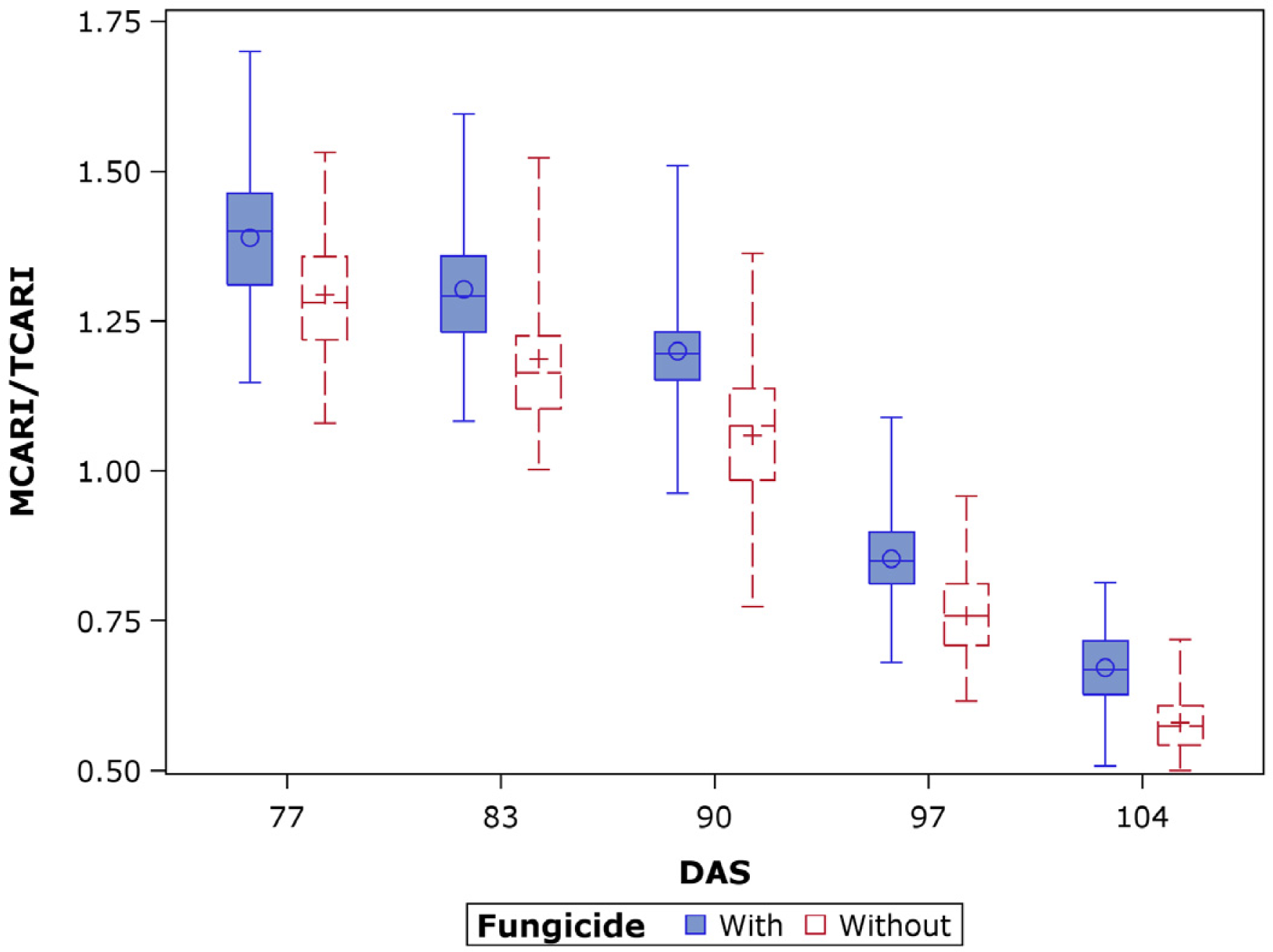
The field experiment of barley (Hordeum vulgare) was conducted at the Institute of Crop Science and Resource Conservation (INRES-Horticultural Science, 50.7299°N, 7.0754°E; 70 m.a.s.l.), University of Bonn, Germany. The soil is sandy loam with the N_min value of 20 kg·N·ha⁻¹. The annual average precipitation and temperature are 669 mm and 10.3 °C, respectively. The experiment was organized as a completely randomized block with three replications and a plot size of 6 m² (4 × 1.5 m) for each variety and fungicide treatment. Ten rows of barley plants sown with a density of 320 seeds per square meter were grown in each plot. The experimental design included seven barley varieties (Belana, Marthe, Scarlett, Iron, Sunshine, Barke and Bambina) and two fungicide variants (with fungicide and without fungicide).

For the treatment group with fungicide, plants were regularly sprayed with protective or curative fungicides over the entire experimental period, while for the treatment group without fungicide no fungicides were sprayed. The seven commercial varieties of malting barley were sown on 24 March 2010. All plots were fertilized immediately after sowing with ammonium nitrate (NH₄⁺-N) at the rate of 100 kg·N·ha⁻¹.

For the plants of without fungicide plots, the infections were generally mild and showed only a few punctiform symptoms due to the unfavorable climatic conditions to pathogens at the study site in 2010.

2.2. Fluorescence Measurements

Random plants were preselected and marked prior to the implementation of treatment design of fungicide. From these plants, six uppermost fully expanded flag leaves were randomly sampled, stored in a cold box and immediately transported into the lab for the fluorescence measurements. The fluorescence recordings were carried out at the beginning of June up to July at weekly intervals on five dates; 9 June (77 DAS, days after sowing), 15 June (83 DAS), 22 June (90 DAS), 29 June (97 DAS) and 6 July (104 DAS). A multi-parametric fluorescence sensor, Multiplex® 3 [41], was used in this study for the recording of fluorescence signals. Barley leaves were placed on a black anodized plate for measuring the fluorescence indices at room temperature in the lab. The mean readings of the six leaves of each plot served as the representative of each plot.

Table 1. Fluorescence indices used in this study.

Index	Description	Formula
SFR_G	Simple Fluorescence Ratio (green excitation)	FRF_G/ RF_G
SFR_R	Simple Fluorescence Ratio (red excitation)	FRF_R/ RF_R
BFRR_UV	Blue-to-Far Red Fluorescence Ratio (UV excitation)	BGF_UV/ FRF_UV
FER_RUV	Fluorescence Excitation Ratio (red & UV excitation)	FRF_R/ FRF_UV
FLAV	Flavonols	log(FER_RUV)
FER_RG	Fluorescence Excitation Ratio (red & green excitation)	FRF_R/ FRF_G
ANTH	Anthocyanins	log(FER_RG)
NBI_G	Nitrogen Balance Index (SFR_G/FER_RUV)	FRF_UV/ RF_G
NBI_R	Nitrogen Balance Index (SFR_R/FER_RUV)	FRF_UV/ RF_R
FERARI	Fluorescence Excitation Ratio Anthocyanin Relative Index	log(1/FRF_R)

presents the ten fluorescence indices that were investigated in this study.

2.3. Hyperspectral Reflectance Measurements

Prior to leaf sampling, canopy reflectance was measured within two hours of solar noon using QualitySpec® Pro (9 June, and 15 June) and FieldSpec® 3 (22 June, 29 June and 6 July) spectrometers from a distance of 1 m above the canopy. The same white reference panel (Spectralon) was used for calibrations for both spectrometers before spectral measurement in the field. In addition, our unpublished results of cross calibration showed that the reflectance difference is negligible, especially for the wavelengths shorter than 1,000 nm because both spectrometers were configured with the same type of detectors (ASD Inc.). The detailed configurations of the spectrometers were described elsewhere [42]. For each of the experiment plots, six reflectance spectra were measured at six random locations within the plot. Finally, reflectance data with 1 nm steps was output for further analysis.

Table 2. Reflectance indices used in this study.

Index	Formula	Reference
PSSRa	R800/R680	Blackburn [43]
ZM	R750/R710	Zarco-Tejada et al. [44]
NPQI	(R415 − R435)/(R415 + R435)	Peñuelas et al. [45]
PRI	(R531 − R570)/(R531 + R570)	Gamon et al. [46]
MCARI	[(R700 − R670) − 0.2 × (R700 − R550)] × (R700/R670)	Daughtry et al. [47]
TCARI	3 × [(R700 − R670) − 0.2 × (R700 − R550) × (R700/R670)]	Haboudane et al. [48]
OSAVI	(1 + 0.16) × (R800 − R670)/(R800 + R670 + 0.16)	Rondeaux et al. [49]
MCARI/OSAVI	MCARI/OSAVI	Daughtry et al. [47]
TCARI/OSAVI	TCARI/OSAVI	Haboudane et al. [48]
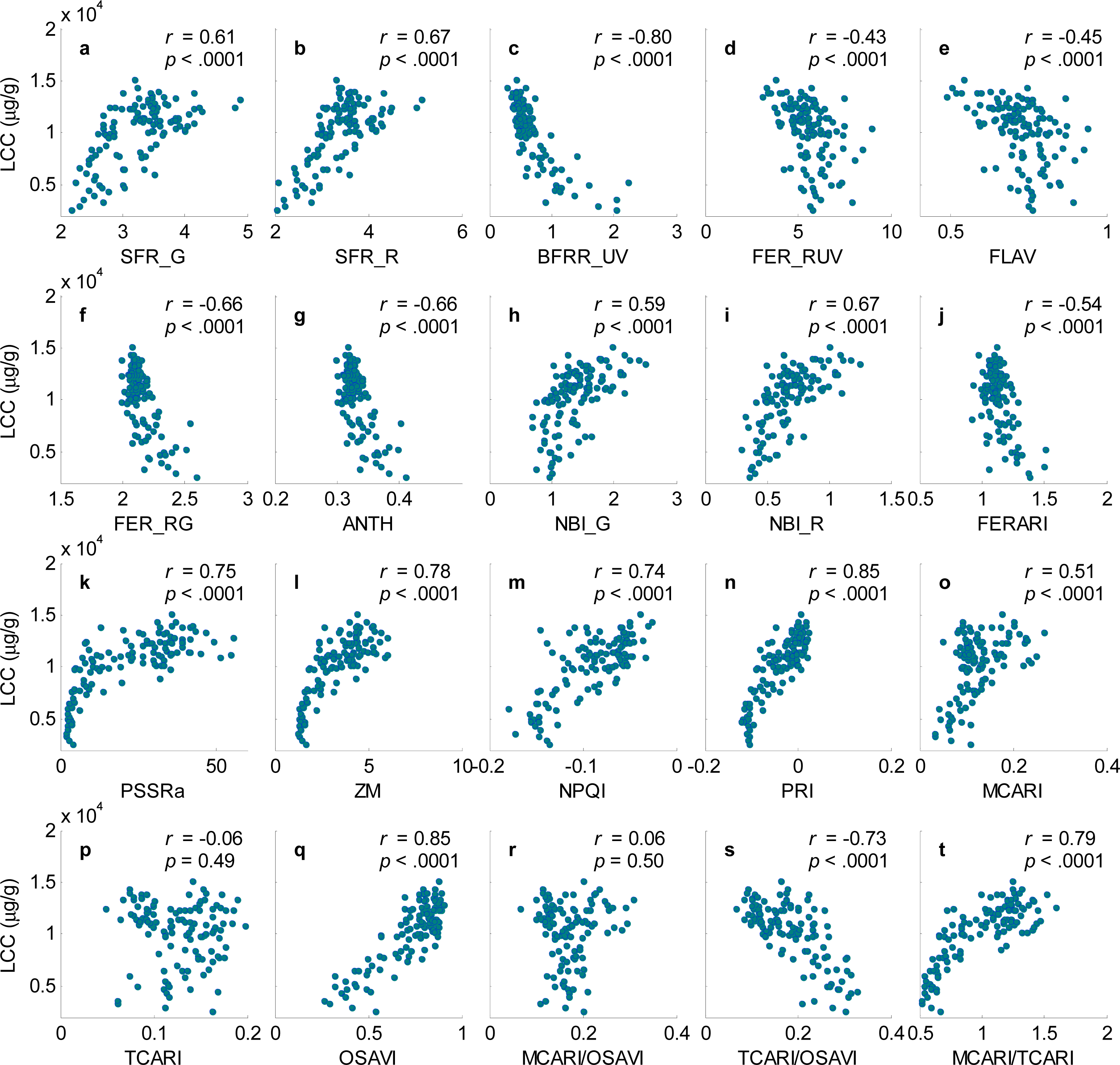
MCARI/TCARI	MCARI/TCARI	Based on [47,48]

shows the ten reflectance indices [43–49] used in this study.

2.4. Leaf Sampling and Chlorophyll Determination

After the fluorescence recordings, the six leaf samples of each plot were immediately frozen, free-dried, grounded and stored in the dark at room temperature for the determination of their chlorophyll content. The total chlorophyll content of each sample was extracted from 50 mg lyophilized material by 5 ml methanol, which was then filled up to 25 ml. After extraction, the absorbance of the extracts was measured with a UV-VIS spectrophotometer (Perkin-Elmer, Lambda 5, Waltham, MA, USA) and the leaf chlorophyll concentration (LCC) was finally determined.

2.5. Data Analysis

2.5.1. Binary Logistic Regression

To detect diseases in the without-fungicide treatment group, binary classification with logistic regression was performed. This method was successfully used in previous studies for detecting scab disease in apple leaves [2,38]. Logistical regression was implemented to examine the ability of each of the fluorescence and reflectance indices (Tables 1 and 2) for detecting the event of interest (disease). Accordingly, the with- and without-fungicide treatment groups correspond respectively to 0 (healthy) and 1 (diseased) in the response variable that represents health status.

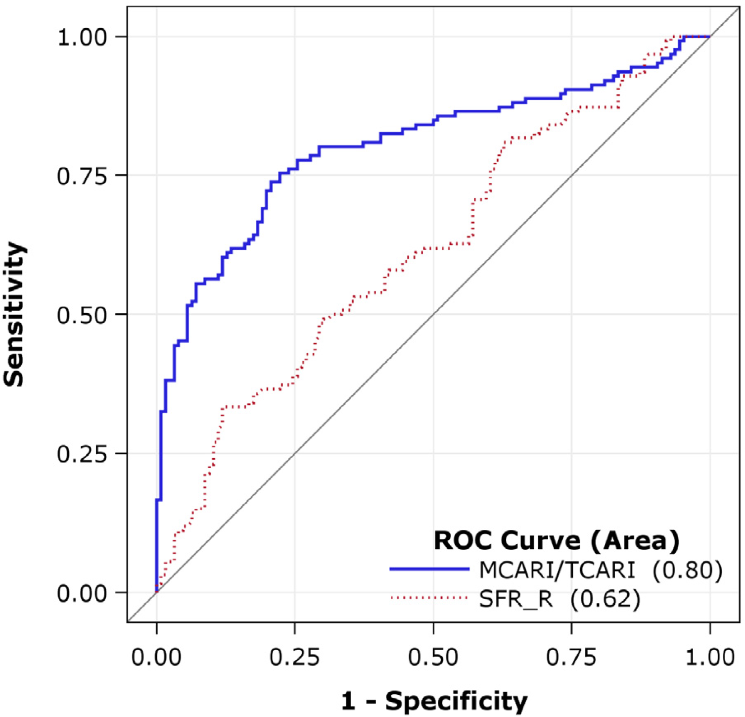
The c-statistic was used to evaluate the discriminatory performance of different indices. The c-value is equivalent to the area under the receiver-operating-characteristic (ROC) curve, and it ranges from 0.5 to 1. The minimum (0.5) and maximum (1) correspond to randomly guessing and perfectly discriminating the response, respectively. The general rule that considers: 0.7 ≤ c < 0.8 as acceptable discrimination; 0.8 ≤ c < 0.9 as excellent discrimination; and c ≥ 0.9 as outstanding discrimination [50] was used to evaluate the discriminatory performance.

2.5.2. Partial Least Squares Regression

The partial least squares (PLS) method was originally developed by the econometrician Herman Wold [51], for use in econometrics for modeling of multivariate time series [52]. The widely used PLS regression (PLSR), which is the simplest PLS approach for linear multivariate modeling, has the advantage that the precision of the model improves with the increasing number of variables and observations [19].

The predictive and response variables are considered as two blocks of variables in the PLSR method [19,53]. The key technique implemented in PLSR is to extract the latent variables (also called factors or components), which serve as new predictors and regress the response variables on these new predictors [54]. These new predictors (hereafter referred to as factors) are expected to explain the variation not only of the response variables but also the predictive variables. How much variation can be explained depends on how many factors are extracted. The more factors that are extracted the more variation can be explained. However, extracting too many factors increases the risk of model overfitting problem (i.e. tailoring the model too much to the training data, leading to the detriment of predicting future observations) [55]. Cross validation is a powerful approach to determine the number of extracted factors through minimizing the prediction error (predicted residual sum of squares, PRESS). However, using the number of factors that yield the minimum in PRESS might also lead to some degree of overfitting [56]. Although various cross validation methods are available, one goal is always preferred that not only a minimum number of factors be selected, but also the risk of overfitting is minimized. To achieve this goal, the statistical model comparison method proposed by van der Voet [57] is implemented. The PLSR model implemented in this study was carried out using the SAS 9.2 software package (SAS Institute Inc.).

2.5.3. Support Vector Regression

The support vector machines (SVM) method is a universal theory of machine learning developed by Vapnik [20]. The main advantage of SVM is its ability to construct a linear function (e.g., classification/regression model) in a high dimensional feature space, where problems of non-linear relations of the training data in the original low dimensional space can be represented, transformed and solved. The support vector regression (SVR) is the implementation of SVM method for regression and function approximation [58] and its standard concept and formulation are briefly described as follows:

Given a training set {(x_i, y_i), ..., (x_l, y_l)}, where x_i ∈ ℝⁿ is a feature vector and y ∈ ℝ is the target output (response variable). Assume that there is a linear function:

$$\widehat{y}=f(x)=\omega \cdot x+b,\hspace{0.17em}\hspace{0.17em}\omega \in {\text{R}}^n,\hspace{0.17em}\hspace{0.17em}\hspace{0.17em}b\in \text{R}$$

(1)

where ŷ is the prediction of y_i, ω is the weight vector and b is the bias. We suppose in Equation (1) the difference between ŷ and y is always extremely small in term of each x_i, i.e., the function f(x) is powerful to predict y. Hence, in order to solve this linear problem of Equation (1) SVR requires the solution of the following optimization problem:

$$\begin{array}{ll}\text{minimize}& \frac{1}{2}{\Vert \omega \Vert }^2\\ \text{subject to}& \Vert y_i-(\omega \cdot x_i-b)\Vert \le \epsilon ,\hspace{0.17em}\hspace{0.17em}\epsilon \ge 0\end{array}$$

(2)

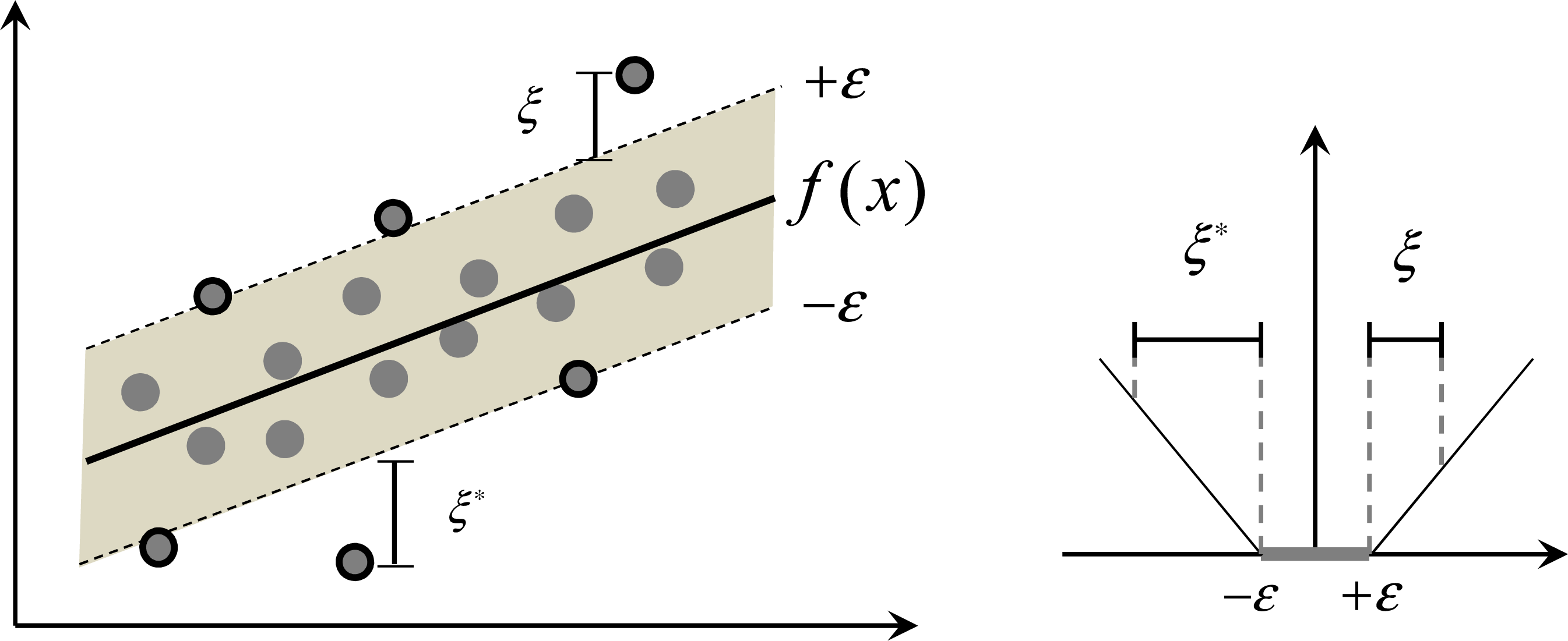
Note that the tacit assumption in Equation (2) was that such a function f(x) does actually exist and that f(x) approximates all pairs (x_i, y_i,) of the training set with the ε precision [58]. This optimization method using ε-insensitive loss function is the widely known ε-SVR [29], which is shown with a schematic in Figure 1. Only the points outside the shaded ε-insensitive tube are called support vectors, which are penalized, and will contribute to the optimization solution [58].

Generally, when ε is under a reasonable range, the optimization problem is considered to be feasible. However, in practical application, it may not be feasible due to different kinds of noises and uncertainty. In this context, the slack variables ξ_i and ${\xi }_i^{*}$ were introduced to permit an otherwise that some instances x_i being out of the ε precision, and then the optimization problem of Equation (2) can be represented as the formulation of the standard form of SVR by Vapnik [20] as follow:

$$\begin{array}{ll}\text{minimize}& \frac{1}{2}{\Vert \omega \Vert }^2+C\sum _{i=1}^l({\xi }_i+{\xi }_i^{*})\\ \text{subject to}& \{\begin{array}{c}{y}_i-\omega \cdot x_i-b\le \epsilon +{\xi }_i\\ \omega \cdot x_i+b-y_i\le \epsilon +{\xi }_i^{*}\\ {\xi }_i,\hspace{0.17em}{\xi }_i^{*}\ge 0\end{array}\end{array}$$

(3)

where (x_i, y_i) has its corresponding ξ_i and ${\xi }_i^{*}$, respectively, which denotes the deviation of predicted value above +ε and below −ε (Figure 1). The parameter C is a constant to determine the tradeoff between the model complexity and the training errors [59]. In addition to the ε-SVR, ν-SVR and some other kinds of SVRs, they vary in the optimization of the corresponding parameters.

Furthermore, based on kernel functions the training data will be mapped into feature space to apply the regression algorithm. Commonly used kernels include linear, polynomial, radial basis function (RBF) and sigmoid. In this study, the ε-SVR model was implemented in MATLAB R2010a (The MathWorks, Inc.) with the LIBSVM tool [60].

2.5.4. Model Validation

The performance of regression models for the estimation of LCC was evaluated by comparing the differences in the coefficients of determination (R²) and root mean square error (RMSE) in predictions. The higher the R² and the lower the RMSE the higher the precision and accuracy of the model to predict LCC. The RMSE values were calculated according to Equation (4),

$$\mathit{RMSE}=\sqrt{\frac{1}{n}\sum _{i=1}^n{(y_i-\widehat{y})}^2}$$

(4)

where y_i and ŷ are the measured and the predicated values of LCC, respectively, and n is the number of samples.

3. Results

3.1. Leaf Chlorophyll Concentration (LCC)

Results of the repeated-measures ANOVA show that both fungicide and variety influenced LCC (

Table 3. Results of repeated-measures ANOVA performed against the leaf chlorophyll concentration (LCC) of barley.

Source	DF	F	P
Fungicide	1	17.63	0.0002
Variety	6	17.10	<0001
Fungicide × Variety	6	1.85	0.1244
Date	4	246.98	<0001
Date × Fungicide	4	3.50	0.0099
Date × Variety	24	1.31	0.1731
Date × Fungicide × Variety	24	0.54	0.9588

). The effect of fungicide treatment on LCC was independent of barley variety (p = 0.12), and vice versa. Sampling date had a significant effect on LCC (p < 0.0001), as well as an interaction with fungicide treatment (p < 0.01). The interaction between the sampling date and variety was not statistically significant (p = 0.17), and the interaction among sampling date, fungicide treatment and variety was not statistically significant (p = 0.96, Table 3).

As expected, LCC was higher on the first two sampling dates (77 and 83 DAS) and decreased as plants aged, irrespective of fungicide treatments (Figure 2). Across all varieties, LCC did not show significant differences between the with- and without-fungicide treatments until the last two sampling dates (97 and 104 DAS), where the LCC was lower in the without-fungicide treatment than the with-fungicide.

3.2. Discriminatory Performances of Fluorescence and Hyperspectral Indices

Table 4. The c statistic showing the performance of fluorescence indices in discriminating between the with- and without-fungicide treatments (bold font highlights c-values that are not less than 0.8).

DAS	Index	Belana	Marthe	Scarlett	Iron	Sunshine	Barke	Bambina	All
77	SFR_G	0.51	0.58	0.62	0.56	0.64	0.70	0.54	0.52
	SFR_R	0.56	0.61	0.60	0.52	0.61	0.67	0.50	0.50
	BFRR_UV	0.69	0.54	0.55	0.54	0.53	0.70	0.62	0.55
	FER_RUV	0.53	0.56	0.51	0.47	0.53	0.73	0.53	0.51
	FLAV	0.54	0.56	0.51	0.53	0.54	0.73	0.54	0.51
	FER_RG	0.57	0.54	0.54	0.54	0.52	0.63	0.57	0.52
	ANTH	0.56	0.54	0.54	0.55	0.52	0.62	0.57	0.53
	NBI_G	0.51	0.50	0.52	0.60	0.52	0.65	0.47	0.52
	NBI_R	0.51	0.52	0.50	0.57	0.52	0.68	0.47	0.52
	FERARI	0.73	0.53	0.60	0.73	0.65	0.72	0.73	0.56
83	SFR_G	0.55	0.65	0.58	0.83	0.55	0.65	0.52	0.61
	SFR_R	0.53	0.65	0.54	0.86	0.59	0.65	0.47	0.62
	BFRR_UV	0.52	0.57	0.62	0.81	0.58	0.67	0.72	0.59
	FER_RUV	0.62	0.58	0.57	0.87	0.54	0.53	0.64	0.55
	FLAV	0.63	0.58	0.57	0.87	0.55	0.53	0.64	0.55
	FER_RG	0.72	0.55	0.60	0.67	0.55	0.64	0.56	0.54
	ANTH	0.72	0.53	0.59	0.66	0.55	0.63	0.56	0.55
	NBI_G	0.64	0.68	0.61	0.70	0.49	0.50	0.60	0.49
	NBI_R	0.67	0.67	0.60	0.71	0.50	0.51	0.61	0.51
	FERARI	0.70	0.54	0.71	0.52	0.68	0.70	0.75	0.58
90	SFR_G	0.52	0.62	0.79	0.61	0.77	0.66	0.55	0.60
	SFR_R	0.54	0.60	0.81	0.60	0.76	0.67	0.51	0.61
	BFRR_UV	0.59	0.54	0.58	0.62	0.60	0.54	0.83	0.54
	FER_RUV	0.50	0.59	0.73	0.53	0.50	0.63	0.79	0.51
	FLAV	0.51	0.59	0.73	0.57	0.53	0.63	0.79	0.51
	FER_RG	0.82	0.68	0.68	0.61	0.62	0.70	0.46	0.62
	ANTH	0.81	0.68	0.67	0.60	0.62	0.71	0.48	0.62
	NBI_G	0.58	0.66	0.54	0.64	0.60	0.47	0.78	0.54
	NBI_R	0.53	0.66	0.56	0.62	0.61	0.55	0.78	0.53
	FERARI	0.65	0.67	0.54	0.58	0.57	0.82	0.89	0.64
97	SFR_G	0.63	0.54	0.65	0.55	0.63	0.67	0.69	0.61
	SFR_R	0.64	0.52	0.65	0.54	0.66	0.68	0.69	0.62
	BFRR_UV	0.82	0.71	0.55	0.65	0.64	0.66	0.88	0.65
	FER_RUV	0.61	0.64	0.68	0.68	0.62	0.58	0.72	0.56
	FLAV	0.61	0.64	0.68	0.68	0.62	0.58	0.72	0.56
	FER_RG	0.52	0.50	0.53	0.50	0.51	0.64	0.54	0.53
	ANTH	0.52	0.49	0.54	0.51	0.51	0.64	0.54	0.53
	NBI_G	0.65	0.61	0.57	0.67	0.60	0.70	0.79	0.60
	NBI_R	0.63	0.62	0.58	0.64	0.59	0.69	0.78	0.59
	FERARI	0.78	0.80	0.62	0.53	0.74	0.67	0.84	0.63
104	SFR_G	0.58	0.65	0.57	0.58	0.56	0.47	0.61	0.53
	SFR_R	0.56	0.63	0.55	0.56	0.53	0.54	0.63	0.51
	BFRR_UV	0.79	0.54	0.52	0.57	0.61	0.69	0.63	0.61
	FER_RUV	0.67	0.50	0.66	0.54	0.72	0.67	0.53	0.59
	FLAV	0.67	0.50	0.65	0.50	0.72	0.67	0.55	0.59
	FER_RG	0.65	0.55	0.49	0.54	0.60	0.70	0.67	0.57
	ANTH	0.65	0.55	0.48	0.54	0.60	0.70	0.67	0.57
	NBI_G	0.56	0.57	0.48	0.46	0.65	0.57	0.42	0.54
	NBI_R	0.62	0.58	0.51	0.45	0.67	0.62	0.61	0.55
	FERARI	0.66	0.54	0.52	0.52	0.61	0.59	0.69	0.57

shows the discriminatory performance of the ten fluorescence indices in discriminating between the with- and without-fungicide treatments. Only few indices performed acceptable (c ≥ 0.7) discrimination for each variety on different sampling dates.

Table 5. The c statistic showing the performance of hyperspectral indices in discriminating between the with- and without-fungicide treatments (bold font and italics highlight c-values that are not less than 0.8 for each variety and for all varieties, respectively).

DAS	Index	Belana	Marthe	Scarlett	Iron	Sunshine	Barke	Bambina	All
77	PSSRa	0.45	0.61	0.52	0.77	0.70	0.80	0.68	0.50
	ZM	0.60	0.72	0.55	0.71	0.67	0.84	0.80	0.57
	NPQI	0.76	0.62	0.72	0.69	0.67	0.79	0.82	0.68
	PRI	0.64	0.56	0.49	0.55	0.58	0.55	0.58	0.46
	MCARI	0.72	0.80	0.59	0.52	0.65	0.87	0.92	0.61
	TCARI	0.65	0.68	0.52	0.54	0.69	0.84	0.83	0.53
	OSAVI	0.72	0.56	0.54	0.63	0.54	0.68	0.45	0.52
	MCARI/OSAVI	0.74	0.81	0.59	0.44	0.65	0.86	0.90	0.62
	TCARI/OSAVI	0.59	0.69	0.51	0.60	0.70	0.84	0.82	0.54
	MCARI/TCARI	0.99	0.90	0.70	0.59	0.56	0.88	0.89	0.73
83	PSSRa	0.59	0.70	0.82	0.99	0.87	0.95	0.85	0.59
	ZM	0.49	0.80	0.77	0.98	0.80	0.94	0.70	0.53
	NPQI	0.71	0.57	0.63	0.61	0.55	0.65	0.74	0.61
	PRI	0.63	0.49	0.82	0.86	0.90	0.75	0.86	0.69
	MCARI	0.85	0.68	0.68	0.54	0.65	0.93	0.79	0.66
	TCARI	0.71	0.49	0.58	0.57	0.68	0.98	0.58	0.55
	OSAVI	0.58	0.62	0.78	0.73	0.74	0.64	0.70	0.59
	MCARI/OSAVI	0.86	0.74	0.64	0.56	0.69	0.93	0.78	0.65
	TCARI/OSAVI	0.69	0.62	0.52	0.65	0.77	0.98	0.54	0.52
	MCARI/TCARI	1.00	0.88	0.95	0.73	0.51	0.81	0.96	0.80
90	PSSRa	0.82	0.51	0.98	1.00	1.00	0.73	1.00	0.77
	ZM	0.65	0.62	0.95	1.00	0.92	0.85	1.00	0.71
	NPQI	0.96	0.74	0.96	0.84	0.58	0.77	0.97	0.78
	PRI	0.86	0.70	0.98	1.00	1.00	0.65	1.00	0.86
	MCARI	1.00	0.75	0.98	0.71	0.55	0.89	0.70	0.80
	TCARI	0.92	0.70	0.84	0.55	0.65	0.90	0.55	0.66
	OSAVI	0.95	0.69	1.00	1.00	0.93	0.65	0.97	0.83
	MCARI/OSAVI	0.99	0.75	0.90	0.49	0.56	0.88	0.56	0.72
	TCARI/OSAVI	0.71	0.71	0.50	0.78	0.76	0.90	0.71	0.53
	MCARI/TCARI	1.00	0.81	1.00	0.90	0.80	0.77	1.00	0.83
97	PSSRa	0.82	0.85	1.00	0.95	0.93	0.97	0.99	0.88
	ZM	0.88	0.81	1.00	1.00	0.95	0.94	1.00	0.88
	NPQI	0.52	0.80	0.85	0.86	0.78	0.88	0.88	0.76
	PRI	0.73	0.88	0.94	0.96	0.96	0.89	0.98	0.89
	MCARI	0.51	0.65	0.90	0.74	1.00	0.84	0.71	0.73
	TCARI	0.77	0.59	0.67	0.63	0.93	0.51	0.50	0.54
	OSAVI	0.77	0.78	1.00	0.99	0.99	0.99	1.00	0.87
	MCARI/OSAVI	0.69	0.52	0.66	0.49	0.97	0.66	0.62	0.56
	TCARI/OSAVI	0.83	0.70	0.74	0.64	0.76	0.72	0.82	0.67
	MCARI/TCARI	0.76	0.86	1.00	0.74	0.77	0.97	0.93	0.82
104	PSSRa	0.77	0.93	1.00	0.99	0.86	0.98	0.96	0.90
	ZM	0.80	0.94	1.00	1.00	0.84	0.98	0.97	0.91
	NPQI	0.72	0.83	0.89	0.90	0.75	0.96	0.86	0.82
	PRI	0.85	0.84	0.62	0.94	0.84	0.90	0.87	0.78
	MCARI	0.78	0.91	1.00	0.94	0.99	0.97	0.93	0.88
	TCARI	0.79	0.88	1.00	0.87	0.96	0.89	0.86	0.85
	OSAVI	0.80	0.94	1.00	0.99	0.93	0.99	0.97	0.91
	MCARI/OSAVI	0.74	0.71	0.97	0.78	0.94	0.60	0.50	0.70
	TCARI/OSAVI	0.50	0.54	0.85	0.50	0.75	0.80	0.78	0.52
	MCARI/TCARI	0.73	0.91	1.00	0.98	0.83	0.98	0.96	0.88

shows the performance of the ten hyperspectral indices in discriminating between the with- and without-fungicide treatments. In most cases, reflectance indices performed significant discrimination (c ≥ 0.8), particularly at later stages. MCARI/TCARI performed best in early stages when across all varieties and yielded acceptable discrimination (c = 0.73) on the first sampling date (77 DAS).

On the first two sampling dates (77 and 83 DAS), SFR_R and MCARI/TCARI yielded the highest c-value compared to other fluorescence and reflectance indices, respectively. Figure 3 shows the ROC curves for the best performing fluorescence index (SFR_R) and reflectance index (MCARI/TCARI) on 83 DAS. MCARI/TCARI and SFR_R yielded the c-value of 0.80 and 0.62, respectively.

Figure 4 shows the performance of MCARI/TCARI on discriminating between the with- and without-fungicide treatments on each sampling date. The without-fungicide treatment yielded significant lower values of MCARI/TCARI than the with-fungicide treatment.

3.3. Relationships between LCC and Fluorescence and Hyperspectral Indices

To compare the performance of different indices for estimating LCC, we divided the whole data into two parts: calibration data consisting of four varieties (Belana, Marthe, Scarlett and Iron) and validation data consisting of another three varieties (Sunshine, Barke and Bambina).

Based on the calibration data, correlation analysis was performed to examine the associations between LCC and the fluorescence and reflectance indices across all sampling dates. As shown in Figure 5, all the fluorescence indices were significantly correlated with the LCC across the sampling dates and varieties (p < 0.0001). The BFRR_UV, SFR_R and NBI_R were the best indices correlating with LCC (Figure 5c,b,i). All reflectance indices were significantly correlated with LCC, with the exception of TCARI (p = 0.49, Figure 5p) and MCARI/OSAVI (p = 0.50, Figure 5r).

3.4. Estimation of LCC

3.4.1. Polynomial Regression Model

Based on the trend of scatter points, second order polynomial regression was used to fit regression models for the three best fluorescence indices (Figure 6a–c) and three best reflectance indices (Figure 6d–f). The validation data set was used to examine the performance of the six indices in predicting LCC.

Table 6. Results of LCC estimations in calibration and validation data sets using SFR_R, BFRR_UV, NBI_R, ZM, PRI, OSAVI, partial least squares regression (PLSR) and support vector regression (SVR) (RMSEc and RMSEv represent root mean square errors for calibration and validation, respectively).

Model	Descriptions	Calibration		Validation
		R2	RMSEc (μg/g)	R2	RMSEv (μg/g)
SFR_R	Polynomial	0.57	1,927.3	0.46	1,863.8
BFRR_UV	Polynomial	0.73	1,524.0	0.72	1,376.3
NBI_R	Polynomial	0.52	2,040.6	0.42	1,952.3
ZM	Polynomial	0.74	1500.9	0.76	1,283.5
PRI	Polynomial	0.75	1,471.8	0.75	1,319.5
OSAVI	Polynomial	0.72	1,549.0	0.79	1,155.5
PLSR	6 Factors	0.84	1,188.1	0.81	1,111.0
SVR	RBF kernel	0.86	1,094.9	0.84	1,021.9

shows the results of the model calibration and validation for each index.

For the calibration data set, SFR_R, BFRR_UV and NBI_R accounted for 57%, 73% and 52% of the variation in LCC, respectively (Table 6). ZM, PRI and OSAVI accounted for 74%, 75% and 72% of the variation in LCC, respectively.

For the validation data set, SFR_R, BFRR_UV and NBI_R models yielded the R² of 0.46, 0.72 and 0.42, respectively. ZM, PRI and OSAVI models yielded the R² of 0.76, 0.75 and 0.79, respectively. Figure 7 shows the comparison between the measured and predicted values of LCC using each of these six indices. BFRR_UV was the best fluorescence index for predicting LCC among the fluorescence indices (Figure 7b). OSAVI was the best reflectance index for predicting LCC among the fluorescence indices (Figure 7f).

3.4.2. PLSR and SVR models

Although fluorescence indices showed acceptable results, SFR_R and NBI_R still failed to account for a large portion (R² < 0.5) of the variation in LCC (Table 6). Therefore, multivariate regression methods were performed to improve the accuracy in estimating LCC using fluorescence signals.

PLSR and SVR models were constructed using all the available fluorescence signals/indices. They explained 84% and 86% of the variation in LCC of calibration data, respectively (Table 6). For the validation data, PLSR and SVR yielded R² of 0.81 and 0.84, respectively. Figure 8 shows that the consistencies between the measured and predicted values of LCC were very high and close to the 1:1 line. SVR slightly outperformed PLSR model for predicting LCC in the calibration and validation data sets. PLSR and SVR models were superior to the fluorescence and reflectance indices (Table 6).

4. Discussion

4.1. Early Detection of the Risk of Disease

Among the five sampling dates, LCC showed significant differences between the with- and without-fungicide treatments only on the last two dates, suggesting that there is a lag of LCC responding to diseases that were mild in this study. Some of the fluorescence indices (recorded on detached leaves) could distinguish between the with- and without-fungicide treatments on the first two sampling dates for some varieties individually, suggesting that fluorescence indices may observe chlorophyll functioning changes that precede significant losses of LCC [37]. Fluorescence indices did not show consistent performance for different varieties on different dates (Table 4), which is due not only to the effect of phenological development [39] but also to variety variations and the mild disease symptoms. Reflectance indices generally showed good performance for distinguish between the with- and without-fungicide plots (Tables 4 and 5). The difference might be related not only to the sensitivity of different indices but also to the measuring methods: while the fluorescence measurement was performed on individual leaves, the reflectance was done from the canopy and could have detected the infections in the leaves of lower layers.

MCARI/TCARI, which is the combination of the Modified Chlorophyll Absorption in Reflectance Index (MCARI) [47] and the Transformed Chlorophyll Absorption in Reflectance Index (TCARI) [48], showed promising performance for discrimination and differentiation between the with- and without-fungicide treatments (Table 5). MCARI was developed for minimizing effects of non-photosynthetic materials [47], based on which TCARI was proposed to counteract the effect of soil background on MCARI [48]. Since diseases affect the absorbed photosynthetically active radiation and thus the radiation use efficiency by leaves, MCARI/TCARI is reasonably expected to detect physiological changes due to diseases, as well as the natural senescence of plant materials. The plants of without-fungicide treatment are also expected to accelerate the senescence process compared to the with-fungicide treatment.

BFRR_UV, as a blue/far-red fluorescence ratio (BF_UV/FRF_UV, Table 1) is considered as a robust indicator of plant stresses [15], however provided excellent (c ≥ 0.8) discrimination for only one variety (Bambina) on the third and fourth sampling dates (90 and 97 DAS) (Table 4). Again, this might be due to that fluorescence measurements were performed on individual leaves rather than the canopy level, as well as for other fluorescence indices.

4.2. Estimation of LCC

Several studies have consistently shown that RF/FRF is a good inverse indicator of the chlorophyll content [10,18,61]. However, our results show that BF/FRF (BFRR_UV) yielded the highest correlation with LCC (Figure 5c), suggesting that the BF/FRF (BFRR_UV) can serve as an indicator of the leaf chlorophyll. Similarly, Heisel et al. [62] found that the BF/FRF (F440/F740) and BF/RF (F440/F690) were more sensitive to the growth conditions than the most frequently used chlorophyll fluorescence ratio RF/FRF (F690/F740).

SFR_G and SFR_R, the FRF/RF ratios that are suggested as chlorophyll indicators by Gitelson et al. [16], were positively correlated to LCC (Figure 6a,b) but yielded lower correlation coefficients as compared to BFRR_UV. This is probably due to (i) different varieties were served as model calibration and validation data sets, (ii) same amount of N fertilizer for each variety. The given conditions could have caused the inconsistency with the previous studies [11,31]. On the other hand, results are consistent to some degree with previous study that the reflectance indices comprised of blue-green and far-red wavelengths are efficient for estimating chlorophyll when across barley varieties [42]. Thus, results reveal that the blue to far-red fluorescence ratio (BF/FRF) might be more useful for modeling LCC across crop varieties. Far-red fluorescence excitation ratios FER_RG and ANTH were also closely related to LCC, which suggests the potential for simultaneously monitoring both chlorophylls and anthocynins using chlorophyll fluorescence [63].

PLS is known as an efficient tool to solve the collinear problems of multivariate statistical analysis [19,22]. Apparently, the fluorescence indices are collinear since the fluorescence ratios are all derived from the measured fluorescence signals (Table 1). Results show that PLSR model provided higher prediction accuracy as compared to the best fluorescence index BFRR_UV (Table 6). Generally, calibration data is expected to have the minimum in predicted residual sum of squares (PRESS). However, a model with fewer factors is always preferred to alleviate the risk of over-fitting. Therefor, 6 factors were extracted for implementing the PLSR model because it satisfied not only the requirement of minimizing PRESS, but also the necessity of statistical tests for none significant increase in the PRESS [57].

SVM has theoretically the advantage for high dimensional data. Similar with previous study [41], nonlinear problems of fluorescence indices also occurred in this study (Figure 6). However, it is critical to determine the proper kernel function in order to produce a good performance and also weaken the complexity of model selection. In this study, the RBF kernel was preferred because RBF kernel outperformed linear and polynomial kernels (data not shown). In addition, RBF kernel not only can handle the case when the relations between dependent variables and predictors are nonlinear but also has fewer numerical difficulties [64].

It is difficult to make a fair comparison between the SVM and the PLS methods. There are more factors and parameters to be carefully considered for the SVM and PLS models as compared to a simple regression method. In this study, SVR model only slightly outperformed PLSR model (Table 6 and Figure 8). Although the consistent result has also been addressed in other studies [65–67], this does not mean that SVR is always the best choice because SVR optimization is relatively slow and complicated compared to PLSR [65]. Overall, SVR and PLSR both seem to be powerful to improve the use of fluorescence signals in estimating LCC.

The relative error of estimation was about 10% for PLSR and SVR, which is low from the practical point of view. The polynomial models using the fluorescence index BFRR_UV was about 13%, which is applicable in practices. However, the multivariate models such as PLS and SVM might be more reliable for future scenarios, where which index is the best choice remains to be studied as shown in the preceding discussion. As the “full spectrum” methods, PLS and SVM not only can deal efficiently with the strong multi-collinearity problem but also consider covariance to the model response/dependent variable(s) [23] when extracting regression factors and support vectors, respectively. Therefore, they are expected to be better adapted to deal with potential confounding factors compared to a simple index-based approach [23].

5. Conclusions

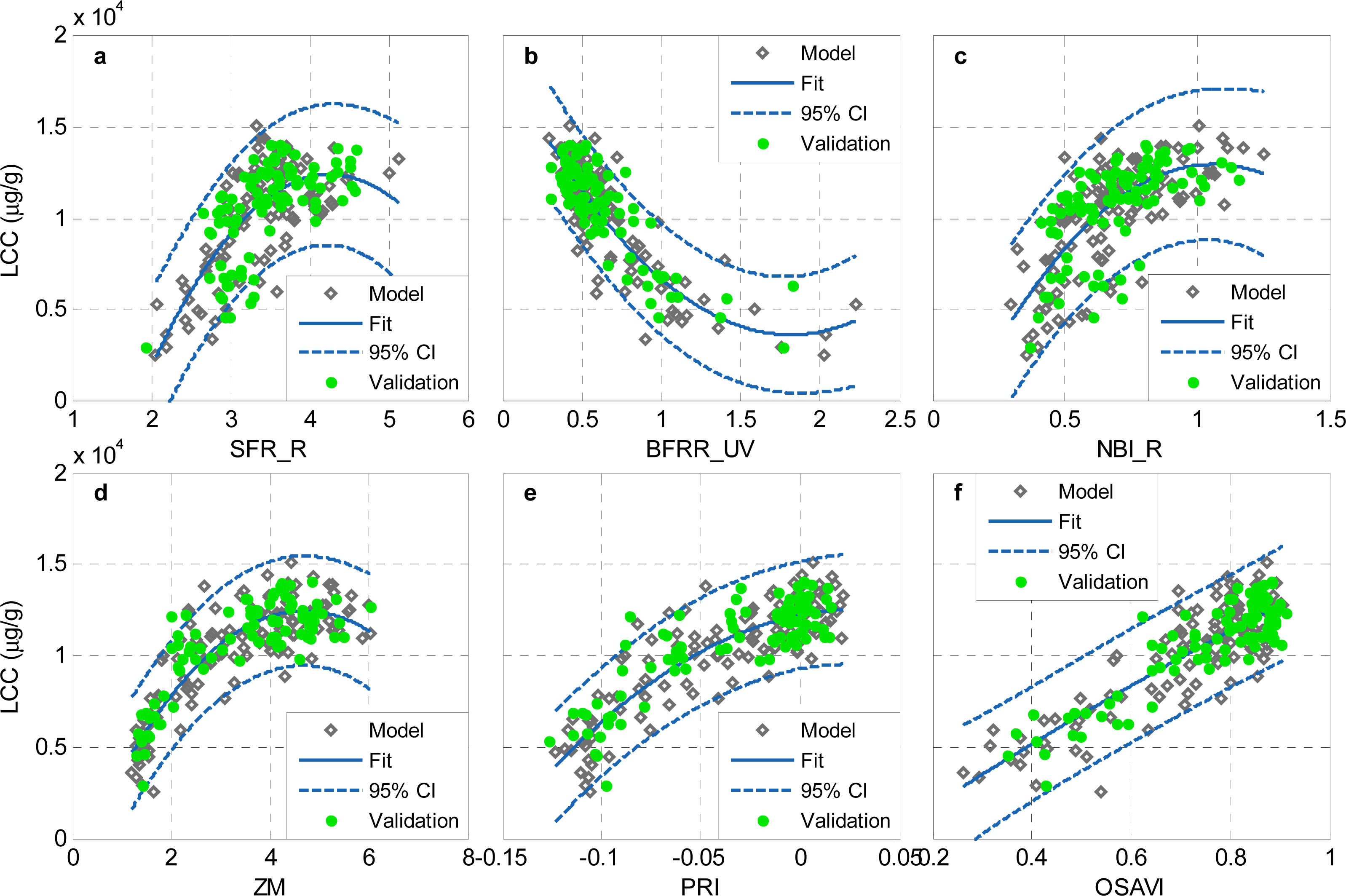
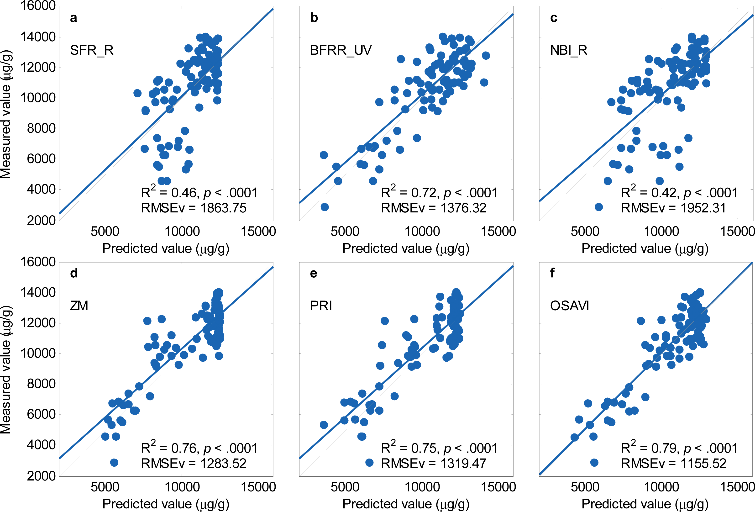
There is a time lag between the occurrence of barley diseases and significant losses of leaf chlorophyll concentration (LCC). Hyperspectral reflectance indices showed good discrimination between healthy and slightly-diseased barley plants that precede significant losses in LCC. A combination of MCARI and TCARI (MCARI/TCARI) showed a promising performance on early detecting diseases across seven barley varieties. Reflectance indices generally showed good performance on predicting LCC (R² = 0.75 − 0.79). The blue to far-red fluorescence ratio, BFRR_UV, also performed well for predicting LCC (R² = 0.72) compared to other fluorescence indices. However, the BFRR_UV vs. LCC relationship was nonlinear, which still constrained the accuracy for LCC estimation. PLSR and SVR models overcome the nonlinear problem, significantly increased the accuracy in estimating LCC (R² > 0.81).

The possible shortage of this study is that fluorescence signals were measured on individual leaves while hyperspectral reflectance were measured on canopy level, thus a meaningful comparison between the fluorescence and reflectance indices is not possible. Future studies should consider performing canopy level fluorescence and hyperspectral measurements for cross comparisons, for example mounting the fluorescence sensor on a wheeled platform [11].

Further studies on different species under different environmental conditions remain to be undertaken to explore the full potential of fluorescence and hyperspectral remote sensing for detecting and identifying crop diseases, which would facilitate the fungicide-specific management in precision agriculture.

References

1. Zarco-Tejada, P.J.; Miller, J.R.; Mohammed, G.H.; Noland, T.L.; Sampson, P.H. Vegetation stress detection through chlorophyll a + b estimation and fluorescence effects on hyperspectral imagery. J. Environ. Qual 2002, 31, 1433–1441. [Google Scholar]
2. Delalieux, S.; van Aardt, J.; Keulemans, W.; Schrevens, E.; Coppin, P. Detection of biotic stress (Venturia inaequalis) in apple trees using hyperspectral data: Non-parametric statistical approaches and physiological implications. Eur. J. Agron 2007, 27, 130–143. [Google Scholar]
3. Bürling, K.; Hunsche, M.; Noga, G. Quantum yield of non-regulated energy dissipation in PSII (Y(NO)) for early detection of leaf rust (Puccinia triticina) infection in susceptible and resistant wheat (Triticum aestivum L.) cultivars. Precis. Agric 2010, 11, 703–716. [Google Scholar]
4. Tremblay, N.; Wang, Z.; Cerovic, Z.G. Sensing crop nitrogen status with fluorescence indicators. A review. Agron. Sustain. Dev 2012, 32, 451–464. [Google Scholar]
5. Chappelle, E.W.; Wood, F.M., Jr.; McMurtrey, J.E., III; Newcomb, W.W. Laser-induced fluorescence of green plants. 1: A technique for the remote detection of plant stress and species differentiation. Appl. Opt 1984, 23, 134–138. [Google Scholar]
6. Chappelle, E.W.; McMurtrey, J.E., III; Wood, F.M., Jr.; Newcomb, W.W. Laser-induced fluorescence of green plants. 2: LIF caused by nutrient deficiencies in corn. Appl. Opt 1984, 23, 139–142. [Google Scholar]
7. Lichtenthaler, H.K. Vegetation stress: An introduction to the stress concept in plants. J. Plant. Physiol 1996, 148, 4–14. [Google Scholar]
8. Lang, M.; Lichtenthaler, H.K.; Sowinska, M.; Heisel, F.; Miehé, J.A. Fluorescence imaging of water and temperature stress in plant leaves. J. Plant. Physiol 1996, 148, 613–621. [Google Scholar]
9. Leufen, G.; Noga, G.; Hunsche, M. Physiological response of sugar beet (Beta vulgaris) genotypes to a temporary water deficit, as evaluated with a multiparameter fluorescence sensor. Acta. Physiol. Plant 2013, 35, 1763–1774. [Google Scholar]
10. Buschmann, C. Variability and application of the chlorophyll fluorescence emission ratio red/far-red of leaves. Photosynth. Res 2007, 92, 261–271. [Google Scholar]
11. Lejealle, S.; Evain, S.; Cerovic, Z.G. Multiplex: A New Diagnostic Tool for Management of Nitrogen Fertilization of Turfgrass. Proceedings of the 10th International Conference on Precision Agriculture, Denver, CO, USA, 18–21 July 2010.
12. Lichtenthaler, H.K.; Babani, F. Light Adaptation and Senescence of the Photosynthetic Apparatus. Changes in Pigment Composition, Chlorophyll Fluorescence Parameters and Photosynthetic Activity. In Chlorophyll a Fluorescence: A Signature of Photosynthesis; Papageorgiou, G.C., Govindjee, Eds.; Springer: Dordrecht, The Netherlands, 2004; Volume 19, pp. 713–736. [Google Scholar]
13. Lichtenthaler, H.K.; Rinderle, U. The role of chlorophyll fluorescence in the detection of stress conditions in plants. CRC Crit. Rev. Anal. Chem 1988, 19, S29–S85. [Google Scholar]
14. Gitelson, A.A.; Buschmann, C.; Lichtenthaler, H.K. Leaf chlorophyll fluorescence corrected for re-absorption by means of absorption and reflectance measurements. J. Plant. Physiol 1998, 152, 283–296. [Google Scholar]
15. Lichtenthaler, H.K.; Miehé, J.A. Fluorescence imaging as a diagnostic tool for plant stress. Trend. Plant. Sci 1997, 2, 316–320. [Google Scholar]
16. Gitelson, A.A.; Buschmann, C.; Lichtenthaler, H.K. The chlorophyll fluorescence ratio F735/F700 as an accurate measure of the chlorophyll content in plants. Remote Sens. Environ 1999, 69, 296–302. [Google Scholar]
17. Babani, F.; Lichtenthaler, H.K. Light-induced and age-dependent development of chloroplasts in etiolated barley leaves as visualized by determination of photosynthetic pigments, CO2 assimilation rates and different kinds of chlorophyll fluorescence ratios. J. Plant. Physiol 1996, 148, 555–566. [Google Scholar]
18. Lichtenthaler, H.K.; Langsdorf, G.; Lenk, S.; Buschmann, C. Chlorophyll fluorescence imaging of photosynthetic activity with the flash-lamp fluorescence imaging system. Photosynthetica 2005, 43, 355–369. [Google Scholar]
19. Wold, S.; Sjöström, M.; Eriksson, L. PLS-regression: A basic tool of chemometrics. Chemometr. Intell. Lab. Syst 2001, 58, 109–130. [Google Scholar]
20. Vapnik, V.N. The Nature of Statistical Learning Theory; Springer-Verlag: New York, NY, USA, 1995. [Google Scholar]
21. Plaza, A.; Benediktsson, J.A.; Boardman, J.W.; Brazile, J.; Bruzzone, L.; Camps-Valls, G.; Chanussot, J.; Fauvel, M.; Gamba, P.; Gualtieri, A.; et al. Recent advances in techniques for hyperspectral image processing. Remote Sens. Environ 2009, 113, S110–S122. [Google Scholar]
22. Hansen, P.M.; Schjoerring, J.K. Reflectance measurement of canopy biomass and nitrogen status in wheat crops using normalized difference vegetation indices and partial least squares regression. Remote Sens. Environ 2003, 86, 542–553. [Google Scholar]
23. Atzberger, C.; Guérif, M.; Baret, F.; Werner, W. Comparative analysis of three chemometric techniques for the spectroradiometric assessment of canopy chlorophyll content in winter wheat. Comput. Electron. Agric 2010, 73, 165–173. [Google Scholar]
24. Zheng, H.; Lu, H.; Zheng, Y.; Lou, H.; Chen, C. Automatic sorting of Chinese jujube (Zizyphus jujuba Mill. cv. ‘hongxing’) using chlorophyll fluorescence and support vector machine. J. Food Eng 2010, 101, 402–408. [Google Scholar]
25. Mountrakis, G.; Im, J.; Ogole, C. Support vector machines in remote sensing: A review. ISPRS J. Photogramm. Remote Sens 2011, 66, 247–259. [Google Scholar]
26. Römer, C.; Bürling, K.; Hunsche, M.; Rumpf, T.; Noga, G.; Plümer, L. Robust fitting of fluorescence spectra for pre-symptomatic wheat leaf rust detection with support vector machines. Comput. Electron. Agric 2011, 79, 180–188. [Google Scholar]
27. Durbha, S.S.; King, R.L.; Younan, N.H. Support vector machines regression for retrieval of leaf area index from multiangle imaging spectroradiometer. Remote Sens. Environ 2007, 107, 348–361. [Google Scholar]
28. Sun, D.; Li, Y.; Wang, Q.; Le, C.; Lv, H.; Huang, C.; Gong, S. A novel support vector regression model to estimate the phycocyanin concentration in turbid inland waters from hyperspectral reflectance. Hydrobiologia 2012, 680, 199–217. [Google Scholar]
29. Vapnik, V.N. Statistical Learning Theory; John Wiley & Sons, Inc: New York, NY, USA, 1998. [Google Scholar]
30. Bürling, K.; Hunsche, M.; Noga, G. Use of blue-green and chlorophyll fluorescence measurements for differentiation between nitrogen deficiency and pathogen infection in winter wheat. J. Plant. Physiol 2011, 168, 1641–1648. [Google Scholar]
31. Zhang, Y.; Tremblay, N.; Zhu, J. A first comparison of Multiplex® for the assessment of corn nitrogen status. J. Food. Agric. Environ 2012, 10, 1008–1016. [Google Scholar]
32. Agati, G.; Foschi, L.; Grossi, N.; Guglielminetti, L.; Cerovic, Z.G.; Volterrani, M. Fluorescence-based versus reflectance proximal sensing of nitrogen content in Paspalum vaginatum and Zoysia matrella turfgrasses. Eur. J. Agron 2013, 45, 39–51. [Google Scholar]
33. Cerovic, Z.G.; Moise, N.; Agati, G.; Latouche, G.; Ben Ghozlen, N.; Meyer, S. New portable optical sensors for the assessment of winegrape phenolic maturity based on berry fluorescence. J. Food Compos. Anal 2008, 21, 650–654. [Google Scholar]
34. Buschmann, C.; Lichtenthaler, H.K. Principles and characteristics of multi-colour fluorescence imaging of plants. J. Plant. Physiol 1998, 152, 297–314. [Google Scholar]
35. Langsdorf, G.; Buschmann, C.; Sowinska, M.; Babani, F.; Mokry, M.; Timmermann, F.; Lichtenthaler, H.K. Multicolour fluorescence imaging of sugar beet leaves with different nitrogen status by flash lamp UV-excitation. Photosynthetica 2000, 38, 539–551. [Google Scholar]
36. Cartelat, A.; Cerovic, Z.G.; Goulas, Y.; Meyer, S.; Lelarge, C.; Prioul, J.L.; Barbottin, A.; Jeuffroy, M.H.; Gate, P.; Agati, G.; et al. Optically assessed contents of leaf polyphenolics and chlorophyll as indicators of nitrogen deficiency in wheat (Triticum aestivum L.). Field Crop. Res 2005, 91, 35–49. [Google Scholar]
37. Zarco-Tejada, P.J.; Miller, J.R.; Mohammed, G.H.; Noland, T.L.; Sampson, P.H. Chlorophyll fluorescence effects on vegetation apparent reflectance: II. Laboratory and airborne canopy-level measurements with hyperspectral data. Remote Sens. Environ 2000, 74, 596–608. [Google Scholar]
38. Delalieux, S.; Auwerkerken, A.; Verstraeten, W.; Somers, B.; Valcke, R.; Lhermitte, S.; Keulemans, J.; Coppin, P. Hyperspectral reflectance and fluorescence imaging to detect scab induced stress in apple leaves. Remote Sens 2009, 1, 858–874. [Google Scholar]
39. Delalieux, S.; Somers, B.; Verstraeten, W.W.; van Aardt, J.A.N.; Keulemans, W.; Coppin, P. Hyperspectral indices to diagnose leaf biotic stress of apple plants, considering leaf phenology. Int. J. Remote Sens 2009, 30, 1887–1912. [Google Scholar]
40. Miphokasap, P.; Honda, K.; Vaiphasa, C.; Souris, M.; Nagai, M. Estimating canopy nitrogen concentration in sugarcane using field imaging spectroscopy. Remote Sens 2012, 4, 1651–1670. [Google Scholar]
41. Ben Ghozlen, N.; Cerovic, Z.G.; Germain, C.; Toutain, S.; Latouche, G. Non-destructive optical monitoring of grape maturation by proximal sensing. Sensors 2010, 10, 10040–10068. [Google Scholar]
42. Yu, K.; Lenz-Wiedemann, V.; Leufen, G.; Hunsche, M.; Noga, G.; Chen, X.; Bareth, G. Assessing hyperspectral vegetation indices for estimating leaf chlorophyll concentration of summer barley. ISPRS Ann. Photogramm. Remote Sens. Spat. Inf. Sci 2012. [Google Scholar] [CrossRef]
43. Blackburn, G.A. Quantifying chlorophylls and carotenoids at leaf and canopy scales: An evaluation of some hyperspectral approaches. Remote Sens. Environ 1998, 66, 273–285. [Google Scholar]
44. Zarco-Tejada, P.J.; Miller, J.R.; Noland, T.L.; Mohammed, G.H.; Sampson, P.H. Scaling-up and model inversion methods with narrowband optical indices for chlorophyll content estimation in closed forest canopies with hyperspectral data. IEEE Trans. Geosci. Remote Sens 2001, 39, 1491–1507. [Google Scholar]
45. Peñuelas, J.; Filella, I.; Lloret, P.; Muñoz, F.; Vilajeliu, M. Reflectance assessment of mite effects on apple trees. Int. J. Remote Sens 1995, 16, 2727–2733. [Google Scholar]
46. Gamon, J.A.; Peñuelas, J.; Field, C.B. A narrow-waveband spectral index that tracks diurnal changes in photosynthetic efficiency. Remote Sens. Environ 1992, 41, 35–44. [Google Scholar]
47. Daughtry, C.S.T.; Walthall, C.L.; Kim, M.S.; de Colstoun, E.B.; McMurtrey, J.E., III. Estimating corn leaf chlorophyll concentration from leaf and canopy reflectance. Remote Sens. Environ 2000, 74, 229–239. [Google Scholar]
48. Haboudane, D.; Miller, J.R.; Tremblay, N.; Zarco-Tejada, P.J.; Dextraze, L. Integrated narrow-band vegetation indices for prediction of crop chlorophyll content for application to precision agriculture. Remote Sens. Environ 2002, 81, 416–426. [Google Scholar]
49. Rondeaux, G.; Steven, M.; Baret, F. Optimization of soil-adjusted vegetation indices. Remote Sens. Environ 1996, 55, 95–107. [Google Scholar]
50. Hosmer, D.W.; Lemeshow, S. Applied Logistic Regression, 2nd ed.; John Wiley & Sons, Inc: New York, NY, USA, 2000. [Google Scholar]
51. Wold, H. Estimation of Principal Components and Related Models by Iterative Least Squares. In Multivariate Analysis; Krishnaiaah, P.R., Ed.; Academic Press: New York, NY, USA, 1966; pp. 391–420. [Google Scholar]
52. Wold, S. Personal memories of the early PLS development. Chemometr. Intell. Lab. Syst 2001, 58, 83–84. [Google Scholar]
53. Wold, S.; Kettaneh-Wold, N.; Skagerberg, B. Nonlinear PLS modeling. Chemometr. Intell. Lab. Syst 1989, 7, 53–65. [Google Scholar]
54. Rosipal, R.; Krämer, N. Overview and Recent Advances in Partial Least Squares. In Subspace, Latent Structure and Feature Selection; Saunders, C., Grobelnik, M., Gunn, S., Shawe-Taylor, J., Eds.; Springer-Verlag: Berlin, Germany, 2006; Volume 3940, pp. 34–51. [Google Scholar]
55. SAS Institute Inc. SAS/STAT® 9.2 User’s Guide; SAS Institute Inc: Cary, NC, USA, 2008. [Google Scholar]
56. Haaland, D.M.; Thomas, E.V. Partial least-squares methods for spectral analyses. 1. Relation to other quantitative calibration methods and the extraction of qualitative information. Anal. Chem 1988, 60, 1193–1202. [Google Scholar]
57. Van der Voet, H. Comparing the predictive accuracy of models using a simple randomization test. Chemometr. Intell. Lab. Syst 1994, 25, 313–323. [Google Scholar]
58. Smola, A.J.; Schölkopf, B. A tutorial on support vector regression. Stat. Comput 2004, 14, 199–222. [Google Scholar]
59. Yang, F.; White, M.A.; Michaelis, A.R.; Ichii, K.; Hashimoto, H.; Votava, P.; Zhu, A.X.; Nemani, R.R. Prediction of continental-scale evapotranspiration by combining MODIS and AmeriFlux data through support vector machine. IEEE Trans. Geosci. Remote Sens 2006, 44, 3452–3461. [Google Scholar]
60. Chang, C.; Lin, C. LIBSVM: A library for support vector machines. ACM Trans. Intell. Syst. Technol 2011, 2, 1–27. [Google Scholar]
61. Ounis, A.; Cerovic, Z.G.; Briantais, J.M.; Moya, I. Dual-excitation FLIDAR for the estimation of epidermal UV absorption in leaves and canopies. Remote Sens. Environ 2001, 76, 33–48. [Google Scholar]
62. Heisel, F.; Sowinska, M.; Miehé, J.A.; Lang, M.; Lichtenthaler, H.K. Detection of nutrient deficiencies of maize by laser induced fluorescence imaging. J. Plant. Physiol 1996, 148, 622–631. [Google Scholar]
63. Agati, G.; Pinelli, P.; Cortes Ebner, S.; Romani, A.; Cartelat, A.; Cerovic, Z.G. Nondestructive evaluation of anthocyanins in Olive (Olea europaea) fruits by in situ chlorophyll fluorescence spectroscopy. J. Agric. Food Chem 2005, 53, 1354–1363. [Google Scholar]
64. Hsu, C.W.; Chang, C.C.; Lin, C.J. A Practical Guide to Support Vector Classification. Available online: http://www.csie.ntu.edu.tw/∼cjlin/papers/guide/guide.pdf (accessed on 1 November 2013).
65. Thissen, U.; Pepers, M.; Üstün, B.; Melssen, W.J.; Buydens, L.M.C. Comparing support vector machines to PLS for spectral regression applications. Chemometr. Intell. Lab. Syst 2004, 73, 169–179. [Google Scholar]
66. Yu, H.; Lin, H.; Xu, H.; Ying, Y.; Li, B.; Pan, X. Prediction of enological parameters and discrimination of rice wine age using least-squares support vector machines and near infrared spectroscopy. J. Agric. Food Chem 2008, 56, 307–313. [Google Scholar]
67. Borin, A.; Ferrão, M.F.; Mello, C.; Maretto, D.A.; Poppi, R.J. Least-squares support vector machines and near infrared spectroscopy for quantification of common adulterants in powdered milk. Anal. Chim. Acta 2006, 579, 25–32. [Google Scholar]
Figure 1. Schematic of linear support vector regression (SVR) and the ε-intensive loss function (circles with black outline are support vectors).
Remotesensing 06 00064f1
Figure 2. Box-and-whiskers plots showing the differences between the with- and without-fungicide treatments across varieties for each sampling date. Significant differences were observed at the last two sampling dates (*, p < 0.05; **, p < 0.01).
Remotesensing 06 00064f2
Figure 3. ROC plot shows the performances of MCARI/TCARI and SFR_R for the discriminating between the with- and without-fungicide treatments at the second sampling date (DAS 83). The area under ROC curves is 0.80 and 0.62 for MCARI/TCARI and SFR_R, respectively.
Remotesensing 06 00064f3
Figure 4. Box-and-whiskers plots showing the significant performance of MCARI/TCARI on discriminating between the with- and without-fungicide treatments. Significant (p < 0.01) differences between the with- and without-fungicide treatments were observed on each sampling date across all varieties (circle and plus signs show the means of the with- and without-fungicide treatments, respectively).
Remotesensing 06 00064f4
Figure 5. Scatter plots showing the relationships between LCC with (a–j) the ten fluorescence indices and (k–t) ten reflectance indices used in this study for the calibration data set.
Remotesensing 06 00064f5
Figure 6. Fitting second order polynomial regression models to the calibration data for (a) SFR_R, (b) BFRR_UV, (c) NBI_R, (d) ZM, (e) PRI and (f) OSAVI and validating each of the indices for predicting LCC using the independent validation data.
Remotesensing 06 00064f6
Figure 7. Measured-by-predicted values of LCC showing the validation results of (a) SFR_R, (b) BFRR_UV, (c) NBI_R, (d) ZM, (e) PRI and (f) OSAVI in predicting the LCC of the validation data set. Solid and dashed lines show the best linear fit and 1:1 lines, respectively.
Remotesensing 06 00064f7
Figure 8. Measured-by-predicted values of LCC showing the validation results of (a) PLSR model and (b) SVR model in predicting the LCC of the validation data set. Solid and dashed lines show the best linear fit and 1:1 lines, respectively.
Remotesensing 06 00064f8