Airborne Dual-Wavelength LiDAR Data for Classifying Land Cover

Abstract

This study demonstrated the potential of using dual-wavelength airborne light detection and ranging (LiDAR) data to classify land cover. Dual-wavelength LiDAR data were acquired from two airborne LiDAR systems that emitted pulses of light in near-infrared (NIR) and middle-infrared (MIR) lasers. The major features of the LiDAR data, such as surface height, echo width, and dual-wavelength amplitude, were used to represent the characteristics of land cover. Based on the major features of land cover, a support vector machine was used to classify six types of suburban land cover: road and gravel, bare soil, low vegetation, high vegetation, roofs, and water bodies. Results show that using dual-wavelength LiDAR-derived information (e.g., amplitudes at NIR and MIR wavelengths) could compensate for the limitations of using single-wavelength LiDAR information (i.e., poor discrimination of low vegetation) when classifying land cover.

1. Introduction

Airborne light detection and ranging (LiDAR), which measures distance by illuminating a target with a laser, is used for the rapid collection of geolocated elevation data from the surface of the earth. The positions of the targets can be obtained based on a positioning and orientation system. Increasing numbers of researchers have used airborne LiDAR data in landscape mapping [1,2]. LiDAR data typically contain 3D spatial point clouds and the intensity of returns (echoes), and its penetration capabilities make it a better system for identifying vegetation compared with photogrammetry. LiDAR systems can automatically classify land cover from geometric properties [1,3]. Moreover, multispectral image and LiDAR data can provide a large amount of spectral and geometric information for land cover classification. The combination of LiDAR data with either multispectral [4–6] or hyperspectral [7] imagery has been demonstrated to improve land cover classification.

Recently, LiDAR technology has been developed into a full-waveform LiDAR system, which can record the complete waveform of a backscattered signal echo [8]. The full-waveform LiDAR collects a continuous signal for each pulse, whereas the discrete-return LiDAR only collects four to five discrete points. Previous studies [8–10] have indicated that waveform LiDAR data record more physical characteristics than discrete-return LiDAR data. These physical characteristics affect the shape of waveforms and potentially benefit the land cover classification. For example, the waveform of an echo is wider on the canopy or ploughed fields than that on the roads [8]. Each waveform is commonly represented by a mixed Gaussian model that is produced using a Gaussian decomposition process [11]. Each return echo is represented by a Gaussian function, and the Gaussian parameters can be used to characterize the physical features of the echoes. For example, the echo width (Gaussian standard deviation) obtained from full-waveform data after decomposition, which is unavailable to discrete-return LiDAR data, has proven useful for land cover classification [12–14]. The signal-processing step extracts various features from the waveforms, such as echo width [14,15], amplitude [15], intensity [15], rise/ fall time [9] and Fourier coefficients [10,16], which are used to classify land cover and identify tree species. Given these useful features, the application of waveform LiDAR data in land cover classification has been demonstrated.

Although most commercial airborne LiDAR systems emit laser radiation at a single wavelength, multi-spectral LiDAR (MSL) systems that emit laser radiation at various wavelengths have been recently developed. Given that the return laser intensities at various wavelengths are combined in the MSL data, these data can then be used to obtain several MSL indices, such as the normalized difference vegetation index (NDVI) [17] and tree structure segmentation [3], which cannot be obtained using single-wavelength LiDAR data [18,19]. Thus, multiple potential applications of MSL systems have been demonstrated. Chlorophyll content retrieval with hyperspectral LiDAR was reported by [20], and NDVI with multispectral LiDAR was studied by [21,22]. Morsdorf et al. [23] simulated an MSL waveform system to demonstrate its ability in capturing a vertical profile of leaf-level physiology. A dual-wavelength LiDAR can separate the canopy from ground returns [24]. The dual-wavelength LiDAR system, a current MSL system, has been used for specific applications, such as measuring coastal water depths by using green and near-infrared (NIR) bathymetric LiDARs [25], measuring NDVI by using red-NIR wavelength LiDARs [26] and measuring the moisture content of vegetation by using NIR and middle-infrared (MIR) wavelength LiDARs [27]. However, most dual-wavelength or MSL systems are commonly used for bench mounted test instruments or experimental terrestrial operations. MSL has not yet been used to measure the land from airborne platforms, as it is still at an experimental stage.

The classification of land cover in regional areas using remote sensing is essential. In this study, airborne dual-wavelength LiDAR data were obtained by combining two commercial airborne LiDAR systems that emit NIR and MIR laser pulses. The results demonstrated the potential of using dual-wavelength airborne LiDAR data to investigate land cover types. The dual-wavelength amplitude information and waveform features were used to classify land cover. A progressive classification test was conducted to demonstrate that using dual-wavelength LiDAR data resulted in more accurate land cover classification than using single-wavelength LiDAR data.

2. Methodology

2.1. Study Area and Remote Sensing Data

Figure 1a shows the study area, Namasha (Namaxia), which is located on a hillside in southern Taiwan. Namasha, which is a famous source of precious wood, is a suburban district in the northeastern part of Kaohsiung City, located upstream of the Kao-ping river watershed (Figure 1a). This area was severely damaged by Typhoon Morakot in 2009. The study area is 0.95 km², with an average elevation and slope of approximately 722 m and 18°, respectively.

Table 1. Configuration of dual-wavelength data in the two light detection and ranging (LiDAR) systems.

	Optech ALTM Pegasus HD400	Riegl LMS-Q680i
Laser wavelength (nm)	1,064	1,550
Pulse width (FWHM, full width at half maximum) (ns)	7	4
Beam divergence (mrad)	0.20	0.50
Field of view (degree)	40	60
Footprint size (m)	0.2 at 1 km	0.5 at 1 km
Pulse rate (kHZ)	150	220
Range accuracy (cm)	1	2
Date of survey	7 October 2011	8 January 2012
Flying height (m)	2,000	1,900
Point density (pts/m2)	1.81	2.07

shows the dual-wavelength data configuration in the two LiDAR systems. LiDAR data were acquired using the Optech ALTM Pegasus HD400 and the Riegl LMS-Q680i systems. The Optech system emits NIR laser pulses at a wavelength of 1,064 nm [28], whereas the Riegl system emits MIR laser pulses at a wavelength of 1,550 nm [29]. The proposed dual-wavelength LiDAR was obtained by integrating two LiDAR systems, because no airborne, dual-wavelength (e.g., NIR-MIR) LiDAR system was currently available. In the experimental period, most land cover did not change in study area. The radiometric correction for each LiDAR system has been determined [30]. Further correction of dual-wavelength LiDAR systems will be considered for advanced usage [31]. The accuracy of the collected LiDAR data can be verified by comparing with independently surveyed ground control points. Both systems yielded horizontal accuracy of less than 0.40 m and vertical accuracy of less than 0.10 m.

An IGI DigiCAM was used in the Riegl LMS-Q680i system to produce an orthoimage. To develop a reference dataset for validating the classification results, we identified six classes of land cover based on this orthoimage. The classes were selected based on the landscape of the test area: road and gravel (R&G), bare soil (SOIL), low vegetation (LV), high vegetation (HV), roofs (ROOF) and water bodies (WATER). R&G comprised the asphalt and gravel along the western side of the river and on the south side of the study area. LV comprised grass, low crops and other vegetation shorter than 2 m. HV comprised vegetation taller than 2 m, such as broadleaf evergreen forests. Water absorbs most of the incoming radiation [32]. This could result in the low intensity of LiDAR return points or few return points from water bodies. In this study, low-intensity points were returned from water bodies in the Optech system, whereas few return points from water bodies were observed in the Riegl system. Studies have applied the LiDAR data from water bodies to delineate the river boundaries [33].

Figure 1b shows the locations of the reference samples used for training and tests. Various classes of land cover within a small area are often mixed. For example, when LV is not dense, SOIL and LV may mix and become difficult to separate. Thus, two rules were used to assess the reference samples. First, the pixels must be clearly recognizable on the reference samples. Second, the reference samples must be pure, containing no more than one class of land cover. For example, an area containing a mixture of grass (LV) and trees (HV) would not be considered a reference sample.

2.2. Data Processing

Figure 2 shows the processes used in the classification model, namely, data processing, data integration, feature selection and classification. Both the Optech and Riegl LiDAR systems can provide waveform data, recording an intensity signal that represents the interactions between the emitted laser and the illuminated objects along the laser path. Multi-return echoes are recorded in the laser waveform information, and the waveform data can be decomposed into individual components to characterize the original waveform and echoes [34]. In the Gaussian decomposition method, which has been widely applied [11,13,14,35], a Gaussian function is used to represent a decomposed component; this method was used in this study to decompose a waveform into individual echo components. After decomposition, a Gaussian mixture representing a waveform with multiple distinct components was obtained. These components were described using three Gaussian parameters, namely, mean, amplitude and standard deviation. The Gaussian mean of each component was combined with the attitude information of the system when the laser was fired to map the 3D coordinates of each object. The echo amplitude and standard deviation were then attached to each 3D component as the attributes of the LiDAR points. The amplitude and standard deviation of the first LiDAR echo are termed “amplitude” and “echo width” hereafter.

2.3. Data Integration and Feature Selection

Most land covers contain one major echo, except trees and building roofs. Only the first-return (echo) extracted from each full waveform was selected to analyze the land cover. To integrate the LiDAR data, the sample points from the two LiDAR systems were interpolated into gridded images at 1-m resolution and integrated for subsequent processing. The moving average in a circle with a 2-m radius was applied for the interpolation. Based on the LiDAR data characteristics, the following features were captured: (1) amplitude; (2) echo width; and (3) surface height from the Riegl and Optech systems. Surface height is the height of the land cover from the ground elevation and the digital surface model (DSM). The ground elevation was obtained from the digital elevation models (DEMs) that were, in turn, obtained by processing the point clouds by using TerraScan (TerraSolid software) and manual procedures. First, the TerraScan was applied to filter out non-ground points automatically. Manual inspection and editing were subsequently conducted to ensure the quality of the ground data points.

Major features were selected using the Bhattacharyya distance (separability) [36], which is widely used in feature selection and extraction studies. For feature selection, the Bhattacharyya distance, B_ij, has been used as a class-separability measurement between two land cover types based on the assumption of multivariate normality, and is expressed as follows:

$${\text{B}}_{\text{ij}}=\frac{1}{8}{\left({\text{M}}_{\text{i}}-{\text{M}}_{\text{j}}\right)}^{\text{T}}\hspace{0.17em}{\left(\frac{{\text{C}}_{\text{i}}+{\text{C}}_{\text{j}}}{2}\right)}^{-1}\hspace{0.17em}\hspace{0.17em}\left({\text{M}}_{\text{i}}-{\text{M}}_{\text{j}}\right)+\frac{1}{2}\text{ln}\hspace{0.17em}\left[\frac{|({\text{C}}_{\text{i}}+{\text{C}}_{\text{j}})/2|}{{(|{\text{C}}_{\text{i}}|\cdot |{\text{C}}_{\text{j}}|)}^{1/2}}\right]$$

(1)

where M_i and C_i are the mean vector and covariance matrices of class i, respectively. The lower values of Bhattacharyya distance represent less separable classes and higher classification errors. Based on the relation between the Bhattacharyya distance and classification error in the graph of [36], the criterion for the Bhattacharyya distance is 1 if the classification error is less than 10%.

2.4. Classification

The support vector machine (SVM), a supervised classification algorithm, is an effective classification method. SVM is capable of mixing data from diverse sources, responding robustly to dimensionality, and effectively functioning non-linearly in remote sensing applications [37]. The kernel of SVM used in this study was the Gaussian radial basis function. The SVM algorithm is implemented by using the functions from MATLAB (R2012a). Six classes (R&G, SOIL, LV, HV, ROOF and WATER) were chosen as the land cover categories. Amplitude, surface height and echo width from Riegl and Optech systems were used as the major features for classification. From the reference (sampling) data, 1% of samples in each class was selected as the training data in the SVM classifier. After the SVM classifier was trained, all reference data, except the training data, were treated as validation data. The various LiDAR feature sets were used for the progressive classification test. The confusion matrices for each feature set were calculated to assess the classification results.

3. Results and Discussion

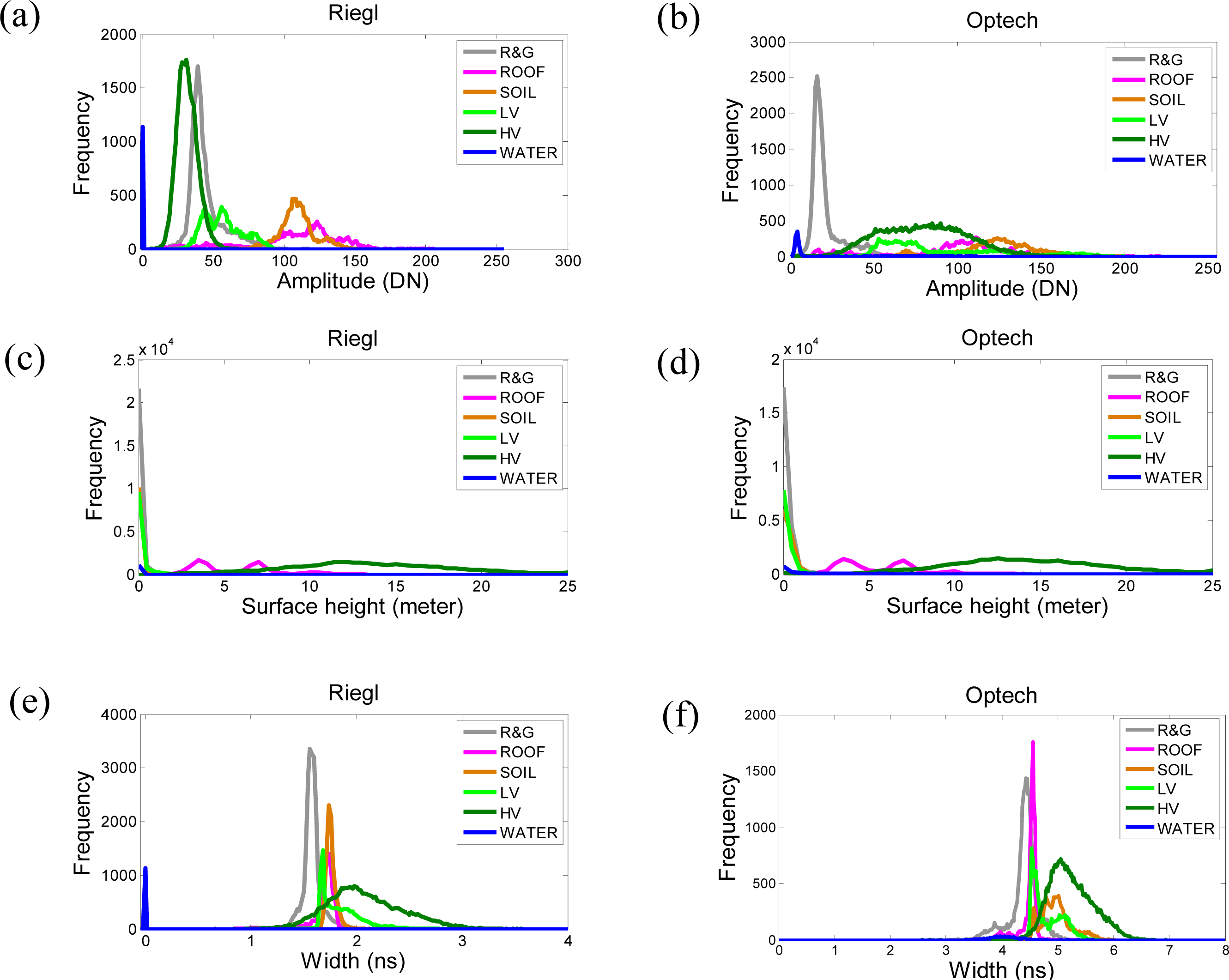
3.1. Analysis of Features

Figure 3 shows the distribution of the amplitude, surface height and echo width of the image pixel elements from the six classes in the reference data. The amplitude values from the Riegl system allowed three groups, namely, WATER, {R&G, LV, HV} and {SOIL, ROOF}, to be distinguished. The amplitude feature from the Optech system improved the separation of WATER, R&G and the remaining classes. The merits of using both amplitudes for classifying land cover are reflected in the accuracy of the preliminary classification. The surface height from the Riegl and Optech systems provided information for separating {R&G, SOIL, LV, WATER} from {HV, ROOF}. The echo width information from the Riegl system indicated two groups, namely WATER, and {R&G, SOIL, LV, HV, ROOF}.

In summary (Figure 3), WATER can be readily classified using most of the features. R&G can be classified using amplitude information from the Optech system. SOIL can be separated from other classes by combining data on amplitude and surface height from the Riegl system. HV can be classified by combining amplitude and surface height information from the Riegl system, and ROOF can be classified by combining all features.

3.2. Feature Selection Using Bhattacharyya Distance

Table 2. Bhattacharyya distance between land cover classes with different feature combinations.

Bhattacharyya Distance Using h *
	R&G	SOIL	LV	HV	ROOF	WATER
R&G	0	0.28 (0.25)	0.00 (0.16)	3.21 (2.52)	2.27 (1.30)	19.52 (0.24)
SOIL		0	0.29 (0.02)	3.79 (3.10)	2.87 (1.94)	18.98 (0.11)
LV			0	3.20 (2.98)	2.26 (1.82)	19.54 (0.15)
HV				0	0.76 (0.92)	23.07 (3.41)
ROOF					0	22.16 (2.31)
WATER						0
Bhattacharyya Distance Using σ *
	R&G	SOIL	LV	HV	ROOF	WATER
R&G	0	0.74 (0.70)	0.48 (0.31)	0.83 (0.56)	0.12 (0.05)	80.07 (0.28)
SOIL		0	0.30 (0.12)	0.85 (0.11)	0.30 (0.60)	301.67 (1.68)
LV			0	0.27 (0.20)	0.11 (0.23)	51.78 (1.06)
HV				0	0.47 (0.54)	28.45 (1.02)
ROOF					0	51.23 (0.53)
WATER						0
Bhattacharyya Distance Using AOptech **
	R&G	SOIL	LV	HV	ROOF	WATER
R&G	0	5.44	1.68	1.06	1.92	2.58
SOIL		0	0.21	0.63	0.14	7.66
LV			0	0.09	0.01	2.88
HV				0	0.14	2.12
ROOF					0	3.15
WATER						0
Bhattacharyya Distance Using ARiegl **
	R&G	SOIL	LV	HV	ROOF	WATER
R&G	0	5.34	0.44	0.29	1.42	28.47
SOIL		0	1.98	7.29	0.18	38.63
LV			0	1.06	0.68	26.63
HV				0	1.81	25.36
ROOF					0	24.70
WATER						0
Bhattacharyya Distance Using ARiegl, AOptech
	R&G	SOIL	LV	HV	ROOF	WATER
R&G	0	8.94	1.69	1.55	2.17	29.98
SOIL		0	2.09	7.36	0.05	40.48
LV			0	1.17	0.48	26.10
HV				0	1.58	25.00
ROOF					0	24.95
WATER						0
Bhattacharyya Distance Using ARiegl, AOptech, h, σ
	R&G	SOIL	LV	HV	ROOF	WATER
R&G	0	9.52	2.34	7.53	4.66	111.44
SOIL		0	2.91	13.79	4.03	376.15
LV			0	5.47	4.42	103.44
HV				0	5.21	56.45
ROOF					0	112.30
WATER						0
Bhattacharyya Distance Using ARiegl, AOptech, h
	R&G	SOIL	LV	HV	ROOF	WATER
R&G	0	8.23	1.70	5.45	3.82	107.14
SOIL		0	2.55	12.07	3.58	60.54
LV			0	4.97	3.39	98.71
HV				0	3.22	46.58
ROOF					0	44.97
WATER						0

^*The surface height (h) and echo width (σ) are from the Riegl system; the number in parentheses represents those from the Optech system.

^**A_Optech, A_Riegl: the Optech and Riegl amplitude information.

lists the Bhattacharyya distances among the classes for different feature sets. The performances of the Riegl and Optech surface height and echo width were consistent. The Riegl surface height and echo width were eventually considered as the major features in the study based on the comparison of Bhattacharyya distance matrix determinants. The matrix determinants of the Riegl surface height and echo width were larger than those of the Optech ones. When the model considered the Riegl surface height information, the classes such as HV and ROOF could be separated from other classes. When the model considered the Riegl echo width information, the Bhattacharyya distances between HV and SOIL and between HV and R&G were 0.85 and 0.83, respectively. The Riegl and Optech systems provided complementary amplitude information for land cover discrimination. When the Optech amplitude information was used, the separability between LV and R&G was 1.68, and 0.21 between LV and SOIL. When the Riegl amplitude information was used, the separability between LV and R&G was 0.44, and 1.98 between LV and SOIL. The same situation in complementary amplitude information occurred between HV and R&G and between HV and SOIL. Compared with the separability values obtained using the Riegl amplitude information, those obtained using the Optech amplitude information were higher for HV and R&G but lower for HV and SOIL. However, when the model considered both sets of amplitude information, the separability between LV and R&G and between LV and SOIL increased. When the model considered both the Riegl and Optech amplitude information, all land cover became separable, except between ROOF and SOIL and between ROOF and LV.

A feature is more critical if the separability among all land cover types is higher. Moreover, feature separability is highly related to classification accuracy. Amplitude is a dominant feature that varies based on the radiometric and geometric properties of the targets [38]. When classifying land cover, the measured amplitudes are high for bare soil and grass and low for water and roads. However, the amplitude varies for high vegetation and roofs of buildings depending on the materials and sensors. LiDAR-based features, such as laser intensity, amplitude, surface height, and topographic data, are primarily used to classify land cover [39]. The feature information of LiDAR data is critical to increase the discriminability of LV and HV classes because the information contains similar spectral signatures [40]. Numerous applications described in the introduction (e.g., chlorophyll or NDVI) are available from dual-wavelength LiDAR data. Future studies should examine the potential of dual-wavelength LiDAR data for extracting the details of vegetation species. When the commercial MSL becomes available for airborne platforms in the future, the MSL instruments will contain many more wavelengths to improve separability. Key information, such as the chlorophyll, NDVI and moisture content, about the vegetation can be derived from MSL data. The applications for vegetation species recognition and forest ecosystem estimation would be expected to benefit from the information.

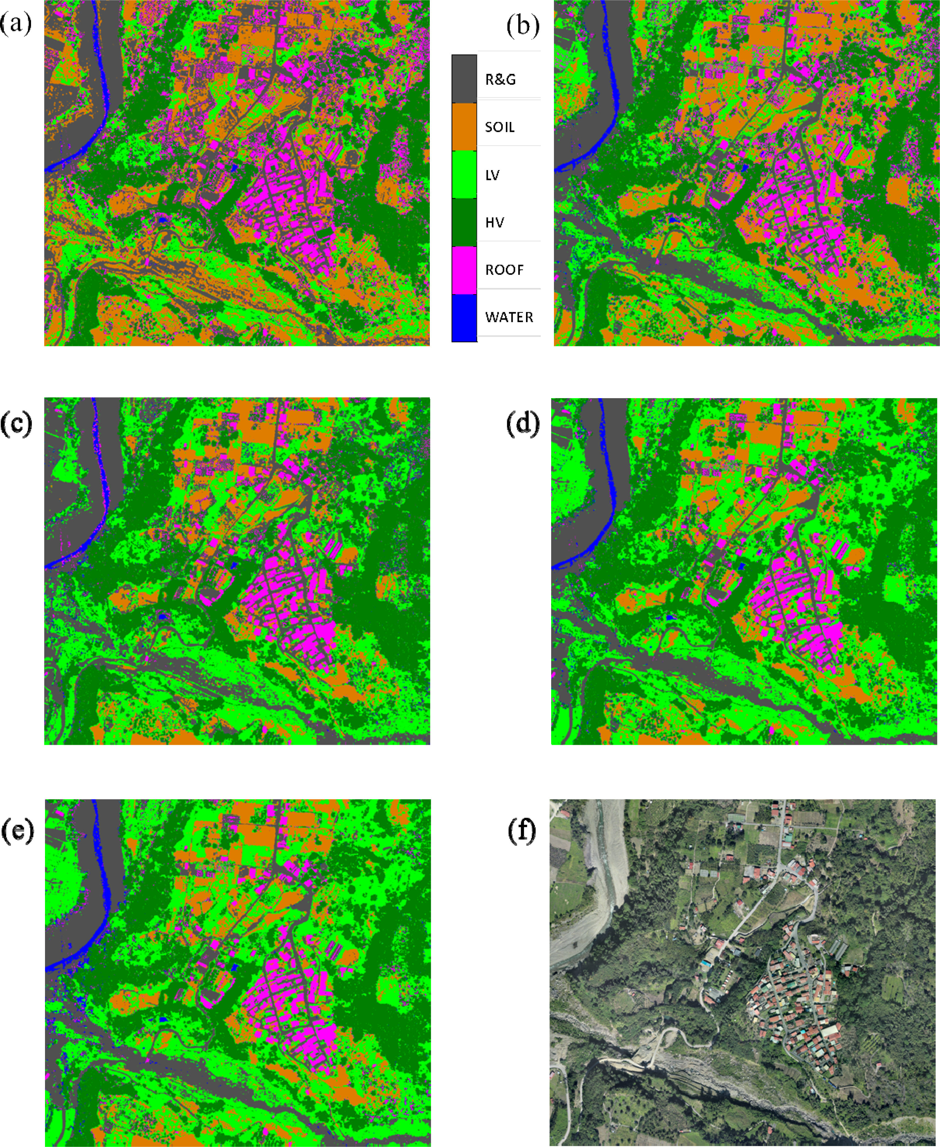
3.3. Classification Accuracies

Table 3. Confusion matrices between the reference and SVM classification using various feature sets. The feature sets are ϕ₁: {h, σ}, ϕ₂: {A_Optech, h, σ}, ϕ₃: {A_Riegl, h, σ}, ϕ₄:{A_Riegl, A_Optech, h, σ } and ϕ₅:{A_Riegl, A_Optech, h }, respectively. The user’s, producer’s and overall accuracies and the Kappa of the classifications are shown. A_Riegl, A_Optech, h, σ

Feature Set	Reference Pixels	Classified Pixels						Producer’s Accuracy (%)
		R&G	SOIL	LV	HV	ROOF	WATER
ϕ1	R&G	21,231	1,731	70	0	23	3	92.07
	SOIL	508	9,758	59	0	2	0	94.49
	LV	3,029	5,174	2,602	3	0	0	24.07
	HV	22	0	166	29,402	1,473	60	94.47
	ROOF	233	0	21	1,001	8,664	8	87.28
	WATER	0	0	0	0	0	1,254	100.00
	User’s accuracy (%)	84.85	58.56	89.17	96.70	85.26	94.64
	Overall accuracy (%)	84.29
	Kappa	0.804
ϕ2	R&G	22,790	14	208	1	4	41	98.84
	SOIL	0	10,275	50	0	2	0	99.50
	LV	409	5,540	4,844	13	0	2	44.82
	HV	19	1	119	30,001	946	37	96.39
	ROOF	193	39	40	974	8,680	1	87.44
	WATER	0	0	0	0	0	1,254	100.00
	User’s accuracy (%)	97.35	64.75	92.07	96.81	90.12	93.93
	Overall accuracy (%)	90.00
	Kappa	0.872
ϕ3	R&G	22,173	259	526	0	91	9	96.16
	SOIL	83	10,230	13	0	1	0	99.06
	LV	3,893	1,301	5,609	2	0	3	51.90
	HV	49	0	228	30,624	192	30	98.40
	ROOF	351	3	10	196	9,365	2	94.34
	WATER	0	0	0	0	0	1,254	100.00
	User’s accuracy (%)	83.52	86.75	87.83	99.36	97.06	96.61
	Overall accuracy (%)	91.63
	Kappa	0.892
ϕ4	R&G	22,924	12	93	0	8	21	99.42
	SOIL	0	10,283	43	0	1	0	99.57
	LV	309	943	9,543	6	0	7	88.30
	HV	30	0	249	30,767	54	23	98.86
	ROOF	360	19	55	14	9,477	2	95.47
	WATER	0	0	0	0	0	1,254	100.00
	User’s accuracy (%)	97.04	91.35	95.59	99.93	99.34	95.94
	Overall accuracy (%)	97.40
	Kappa	0.966
ϕ5	R&G	22,942	24	73	1	1	17	99.50
	SOIL	0	10,289	38	0	0	0	99.63
	LV	307	869	9,631	0	0	1	89.11
	HV	8	0	251	30,702	131	31	98.65
	ROOF	658	79	41	204	8,944	1	90.10
	WATER	0	0	0	0	0	1,254	100.00
	User’s accuracy (%)	95.93	91.37	95.98	99.34	98.55	96.17
	Overall accuracy (%)	96.84
	Kappa	0.959

shows the confusion matrices of the classification results using various feature sets. Based on the feature set, ϕ₁, which comprised the surface height and echo width, the overall accuracy of the classification reached 84.29%. However, the level of producer accuracy was extremely low for LV, and many LV pixels were misclassified into R&G and SOIL. Thus, the user accuracy was poor for R&G and SOIL. For the other classes (R&G, SOIL, HV, ROOF and WATER), the feature set, ϕ₁, provided sufficient information for classification. Based on the feature set, ϕ₂, including additional Optech LiDAR amplitude information, the overall accuracy reached 90.00%. By considering Riegl amplitude features, surface height and echo width in the feature set, ϕ₃, the overall accuracy reached 91.63%. LV was misclassified as R&G more frequently using Riegl amplitude information compared with using Optech amplitude information. However, SOIL was misclassified less using the Riegl amplitude than it was using the Optech amplitude (Table 3). User accuracy in separating SOIL and ROOF was higher using the Riegl amplitude than it was using the Optech amplitude, whereas user accuracy for R&G and LV was higher using the Optech amplitude information compared with using the Riegl amplitude information.

When the feature set, ϕ₄ (surface height, echo width and dual-wavelength amplitude), was used, the overall classification accuracy substantially increased compared with using a single system. When ϕ₄ was used, the producer accuracy for LV increased to 88.3% from 44.82% and 51.90% for single systems, and both the overall producer and user accuracies exceeded 90%, except the LV producer accuracy. The overall accuracy (97.4%) and Kappa (0.966) values were highest when features including the dual-wavelength amplitude were used. Without considering the echo width in ϕ₅ (surface height and dual-wavelength amplitude), the overall accuracy decreased to 96.8% and the Kappa value decreased to 0.959. Thus, the echo width could be discarded because of its low effect on the classification. Figure 4 shows the land cover classification results based on various datasets. Most land covers were classified more accurately. These results indicate the effectiveness of using dual-wavelength airborne LiDAR data to classify land cover (Figure 4). Given that the reflectance of land cover objects varies based on wavelength, land cover objects (e.g., LV and HV, SOIL and LV) cannot be readily distinguished when amplitude information is used at a single wavelength. The features of dual-wavelength data are primarily responsible for the improvement in land cover classification demonstrated in this study.

The use of dual-wavelength LiDAR data offers effective geometry information to classify land cover. First, LiDAR data can provide 3D information. Thus, the DSM, DEM, and surface height can be directly obtained. Second, LiDAR data can record multiple returns in forest areas. The canopy reflectance information in spectral images is considerably influenced by the objects under the canopy. Dual-wavelength LiDAR amplitude and geometric information for the canopy, understory vegetation, soil, and other land cover types precisely represent the features of these covers. By contrast, based on the spectral image, the canopy signal cannot be readily separated from that of the understory vegetation and soil. Thus, the LiDAR data are potentially useful in classifying 3D tree species. Third, current LiDAR systems can record waveform data that allow physical features to be extracted, such as the echo width used in this study. These features cannot be obtained from discrete-return LiDAR. All these features, including dual-wavelength amplitude features, facilitate land cover classification, as clearly demonstrated by the current findings. Therefore, this study revealed the potential of dual-wavelength LiDAR applications, which can be developed when airborne LiDAR systems become available. From a practical perspective, the combination of LiDAR and multi-spectral images will be useful for land cover classification.

4. Conclusion

In this study, two airborne LiDAR systems were used to obtain dual-wavelength LiDAR data (i.e., amplitudes at NIR and MIR wavelengths) and classify land cover. The proposed processes involved waveform data processing, data integration, feature selection, and land cover classification. The findings show that using dual-wavelength airborne LiDAR systems could substantially improve land cover classification in large areas compared with using single-wavelength LiDAR. The dual-wavelength amplitude features facilitated the identification of vegetation, particularly LV, more accurately compared with using single-wavelength amplitude.

Based on the major features of LiDAR data, land cover was effectively classified in the absence of auxiliary remote sensing data, and the overall classification accuracy reached 97.4%. Additional applications can be designed for this method in the future until airborne dual-wavelength LiDAR systems are developed.

References

1. Korpela, I.S. Mapping of understory lichens with airborne discrete-return LiDAR data. Remote Sens. Environ 2008, 112, 3891–3897. [Google Scholar]
2. Miliaresis, G.; Kokkas, N. Segmentation and object-based classification for the extraction of the building class from LIDAR DEMs. Comput. Geosci 2007, 33, 1076–1087. [Google Scholar]
3. Suomalainen, J.; Hakala, T.; Kaartinen, H.; Räikkönen, E.; Kaasalainen, S. Demonstration of a virtual active hyperspectral LiDAR in automated point cloud classification. ISPRS J. Photogramm. Remote Sens 2011, 66, 637–641. [Google Scholar]
4. Bork, E.W.; Su, J.G. Integrating LIDAR data and multispectral imagery for enhanced classification of rangeland vegetation: A meta analysis. Remote Sens. Environ 2007, 111, 11–24. [Google Scholar]
5. Hellesen, T.; Matikainen, L. An object-based approach for mapping shrub and tree cover on grassland habitats by use of LiDAR and CIR orthoimages. Remote Sens 2013, 5, 558–583. [Google Scholar]
6. Hartfield, K.A.; Landau, K.I.; van Leeuwen, W.J.D. Fusion of high resolution aerial multispectral and LiDAR data: Land cover in the context of urban mosquito habitat. Remote Sens 2011, 3, 2364–2383. [Google Scholar]
7. Dalponte, M.; Bruzzone, L.; Gianelle, D. Fusion of hyperspectral and LIDAR remote sensing data for classification of complex forest areas. IEEE Trans. Geosci. Remote Sens 2008, 46, 1416–1427. [Google Scholar]
8. Mallet, C.; Bretar, F. Full-waveform topographic lidar: State-of-the-art. ISPRS J. Photogramm. Remote Sens 2009, 64, 1–16. [Google Scholar]
9. Neuenschwander, A.L.; Magruder, L.A.; Tyler, M. Landcover classification of small-footprint, full-waveform lidar data. J. Appl. Remote Sens 2009, 3. [Google Scholar] [CrossRef]
10. Vaughn, N.R.; Moskal, L.M.; Turnblom, E.C. Fourier transformation of waveform Lidar for species recognition. Remote Sens. Lett 2011, 2, 347–356. [Google Scholar]
11. Wagner, W.; Ullrich, A.; Ducic, V.; Melzer, T.; Studnicka, N. Gaussian decomposition and calibration of a novel small-footprint full-waveform digitising airborne laser scanner. ISPRS J. Photogramm. Remote Sens 2006, 60, 100–112. [Google Scholar]
12. Alexander, C.; Tansey, K.; Kaduk, J.; Holland, D.; Tate, N.J. Backscatter coefficient as an attribute for the classification of full-waveform airborne laser scanning data in urban areas. ISPRS J. Photogramm. Remote Sens 2010, 65, 423–432. [Google Scholar]
13. Wagner, W.; Hollaus, M.; Briese, C.; Ducic, V. 3D vegetation mapping using small-footprint full-waveform airborne laser scanners. Int. J. Remote Sens 2008, 29, 1433–1452. [Google Scholar]
14. Hollaus, M.; Aubrecht, C.; Höfle, B.; Steinnocher, K.; Wagner, W. Roughness mapping on various vertical scales based on full-waveform airborne laser scanning data. Remote Sens 2011, 3, 503–523. [Google Scholar]
15. Heinzel, J.; Koch, B. Exploring full-waveform LiDAR parameters for tree species classification. Int. J. Appl. Earth Obs. Geoinf 2011, 13, 152–160. [Google Scholar]
16. Vaughn, N.R.; Moskal, L.M.; Turnblom, E.C. Tree species detection accuracies using discrete point lidar and airborne waveform lidar. Remote Sens 2012, 4, 377–403. [Google Scholar]
17. Wei, G.; Shalei, S.; Bo, Z.; Shuo, S.; Faquan, L.; Xuewu, C. Multi-wavelength canopy LiDAR for remote sensing of vegetation: Design and system performance. ISPRS J. Photogramm. Remote Sens 2012, 69, 1–9. [Google Scholar]
18. Rall, J.A.R.; Knox, R.G. Spectral ratio biospheric lidar. Proceedings of the 2004 IEEE International, Geoscience and Remote Sensing Symposium, 2004, IGARSS’04, Anchorage, AK, USA, 20–24 September 2004; 3, pp. 1951–1954.
19. Kaasalainen, S.; Lindroos, T.; Hyyppa, J. Toward hyperspectral lidar: Measurement of spectral backscatter intensity with a supercontinuum laser source. IEEE Geosci. Remote Sens. Lett 2007, 4, 211–215. [Google Scholar]
20. Hakala, T.; Suomalainen, J.; Kaasalainen, S.; Chen, Y. Full waveform hyperspectral LiDAR for terrestrial laser scanning. Opt. Express 2012, 20, 7119–7127. [Google Scholar]
21. Woodhouse, I.H.; Nichol, C.; Sinclair, P.; Jack, J.; Morsdorf, F.; Malthus, T.J.; Patenaude, G. A multispectral canopy liDAR demonstrator project. IEEE Geosci. Remote Sens. Lett 2011, 8, 839–843. [Google Scholar]
22. Wallace, A.; Nichol, C.; Woodhouse, I. Recovery of forest canopy parameters by Inversion of multispectral LiDAR data. Remote Sens 2012, 4, 509–531. [Google Scholar]
23. Morsdorf, F.; Nichol, C.; Malthus, T.; Woodhouse, I.H. Assessing forest structural and physiological information content of multi-spectral LiDAR waveforms by radiative transfer modelling. Remote Sens. Environ 2009, 113, 2152–2163. [Google Scholar]
24. Hancock, S.; Lewis, P.; Foster, M.; Disney, M.; Muller, J.-P. Measuring forests with dual wavelength lidar: A simulation study over topography. Agric. For. Meteorol 2012, 161, 123–133. [Google Scholar]
25. Irish, J.L.; Lillycrop, W.J. Scanning laser mapping of the coastal zone: The SHOALS system. ISPRS J. Photogramm. Remote Sens 1999, 54, 123–129. [Google Scholar]
26. Chen, Y.; Raikkonen, E.; Kaasalainen, S.; Suomalainen, J.; Hakala, T.; Hyyppa, J.; Chen, R. Two-channel hyperspectral LiDAR with a supercontinuum laser source. Sensors 2010, 10, 7057–7066. [Google Scholar]
27. Gaulton, R.; Danson, F.M.; Ramirez, F.A.; Gunawan, O. The potential of dual-wavelength laser scanning for estimating vegetation moisture content. Remote Sens. Environ 2013, 132, 32–39. [Google Scholar]
28. Optech. Airborne Surveying. Available online: http://www.optech.ca/ (accessed on 20 March 2011).
29. Riegl Laser Measurement Systems. Products of Airborne Scanning. Available online: http://www.riegl.com/ (accessed on 20 March 2011).
30. Höfle, B.; Pfeifer, N. Correction of laser scanning intensity data: Data and model-driven approaches. ISPRS J. Photogramm. Remote Sens 2007, 62, 415–433. [Google Scholar]
31. Briese, C.; Pfennigbauer, M.; Lehner, H.; Ullrich, A.; Wagner, W.; Pfeifer, N. Radiometric calibration of multi-wavelength airborne laser scanning data. Proceedings of the ISPRS Annals of the Photogrammetry, Remote Sensing and Spatial Information Sciences, XXII ISPRS Congress, Melbourne, Australia, 25 August–1 September 2012.
32. Antonarakis, A.S.; Richards, K.S.; Brasington, J. Object-based land cover classification using airborne LiDAR. Remote Sens. Environ 2008, 112, 2988–2998. [Google Scholar]
33. Cobby, D.M.; Mason, D.C.; Davenport, I.J. Image processing of airborne scanning laser altimetry data for improved river flood modelling. ISPRS J. Photogramm. Remote Sens 2001, 56, 121–138. [Google Scholar]
34. Jinha, J.; Crawford, M.M. Extraction of features from LIDAR waveform data for characterizing forest structure. IEEE Geosci. Remote Sens. Lett 2012, 9, 492–496. [Google Scholar]
35. Reitberger, J.; Schnörr, C.; Krzystek, P.; Stilla, U. 3D segmentation of single trees exploiting full waveform LIDAR data. ISPRS J. Photogramm. Remote Sens 2009, 64, 561–574. [Google Scholar]
36. Choi, E.; Lee, C. Feature extraction based on the Bhattacharyya distance. Pattern Recognit 2003, 36, 1703–1709. [Google Scholar]
37. Bretar, F.; Chauve, A.; Bailly, J.S.; Mallet, C.; Jacome, A. Terrain surfaces and 3-D landcover classification from small footprint full-waveform lidar data: Application to badlands. Hydrol. Earth Syst. Sci 2009, 13, 1531–1544. [Google Scholar]
38. Mallet, C.; Bretar, F.; Roux, M.; Soergel, U.; Heipke, C. Relevance assessment of full-waveform lidar data for urban area classification. ISPRS J. Photogramm. Remote Sens 2011, 66, S71–S84. [Google Scholar]
39. Ke, Y.; Quackenbush, L.J.; Im, J. Synergistic use of QuickBird multispectral imagery and LIDAR data for object-based forest species classification. Remote Sens. Environ 2010, 114, 1141–1154. [Google Scholar]
40. Tooke, T.R.; Coops, N.C.; Goodwin, N.R.; Voogt, J.A. Extracting urban vegetation characteristics using spectral mixture analysis and decision tree classifications. Remote Sens. Environ 2009, 113, 398–407. [Google Scholar]
Figure 1. (a) Location of the study area; (b) location of the reference data for classification.
Remotesensing 06 00700f1
Figure 2. Flowchart of the approach. DSM, digital surface model; DEM, digital elevation model; SVM, support vector machine; HV, high vegetation; LV, low vegetation; SOIL, bare soil; ROOF, roofs; R&G, road and gravel.
Remotesensing 06 00700f2
Figure 3. Frequency distribution of (a) the amplitude from the Riegl system, (b) the amplitude from the Optech system, (c) the surface height from the Riegl system, (d) the surface height from the Optech system, (e) the echo width from the Riegl system and (f) the echo width from the Optech system.
Remotesensing 06 00700f3
Figure 4. Results of the classifications using the five feature sets: (a) Riegl surface height, echo width (set ϕ1); (b) Optech amplitude, Riegl surface height, echo width (set ϕ2); (c) Riegl amplitude, Riegl surface height, echo width (set ϕ3); (d) Riegl amplitude, Optech amplitude, Riegl surface height, echo width (set ϕ4); (e) Riegl amplitude, Optech amplitude, Riegl surface height (set ϕ5); and (f) the orthoimage.
Remotesensing 06 00700f4