Article

Mapping Forest Degradation due to Selective Logging by Means of Time Series Analysis: Case Studies in Central Africa

Remote Sensing and Geoinformation, Institute for Information and Communication Technologies, Joanneum Research, Steyrergasse 17, A-8010 Graz, Austria
*
Author to whom correspondence should be addressed.
Remote Sens. 2014, 6(1), 756-775; https://doi.org/10.3390/rs6010756
Submission received: 20 November 2013 / Revised: 23 December 2013 / Accepted: 30 December 2013 / Published: 9 January 2014

Abstract

:
Detecting and monitoring forest degradation in the tropics has implications for various fields of interest (biodiversity, emission calculations, self-sustenance of indigenous communities, timber exploitation). However, remote-sensing-based detection of forest degradation is difficult, as these subtle degradation signals are not easy to detect in the first place and quickly lost over time due to fast re-vegetation. To overcome these shortcomings, a time series analysis has been developed to map and monitor forest degradation over a longer period of time, with frequent updates based on Landsat data. This time series approach helps to reduce both the commission and the omission errors compared to, e.g., bi- or tri-temporal assessments. The approach involves a series of pre-processing steps, such as geometric and radiometric adjustments, followed by spectral mixture analysis and classification of spectral curves. The resulting pixel-based classification is then aggregated to degradation areas. The method was developed on a study site in Cameroon and applied to a second site in Central African Republic. For both areas, the results were finally evaluated against visual interpretation of very high-resolution optical imagery. Results show overall accuracies in both study sites above 85% for mapping degradation areas with the presented methods.

1. Introduction

The need to conduct research on tropical forest degradation emerged in the 1990s as the spatial extent of selective logging and fire damage was found to be not accounted for in deforestation studies. Selective logging has a strong impact on the whole forest ecosystem with damage to remaining trees, changes in plant and animal species diversity, impacts on the soil, and also on carbon storage [14]. With regard to carbon storage, in the frame of the Kyoto protocol, reducing emissions from deforestation and degradation in developing countries (REDD) was adopted as a mechanism for the post-Kyoto reporting. The need to address and monitor degradation, along with deforestation, has been emphasized on numerous occasions, such as at the COP meeting in Bali, 2007 (FCCC/CP/2007/6), where the parties “acknowledge that forest degradation also leads to emissions, and needs to be addressed when reducing emissions from deforestation”. In the Congo basin, degradation is considered even more important than, for example, in Latin America or Asia, thus, the “COMIFAC (Commission de Forêts d’Afrique Central) position on the international issue on REDD” calls for “factoring of degradation as much as deforestation in emission calculations”. It has been noted that “estimating degradation is difficult because of the great variability in the forms, factors and degrees of human impact” [5]. Many definitions of forest degradation exist in the literature. A selection of definitions is provided on the FAO website [6]. As no common definition has yet been agreed upon within the REDD+ monitoring system [7], a forest degradation area in this study is defined as an area affected by forest canopy disturbance in terms of gaps, logging roads and skid trails, and where no distinction is made between man-made and natural gaps. The complex nature of forest degradation patterns, quick re-growth, and the frequent cloud cover in tropical areas, have been identified as the main obstacles when mapping tropical forest disturbances.

2. State-of-the-Art

Early studies in the Amazon basin investigated the degradation mapping potential of Landsat imagery by applying visual interpretation [1,8]. Extensive studies in Central Africa used Landsat imagery from three decades to derive area estimates of land cover change by combining a systematic regional sampling scheme, based on high-spatial-resolution imagery with object-based unsupervised classification techniques [9] to track the progression of logging roads. Higher resolution data has been used to track skid trails and tree felling [10]. An overview of different remote sensing methods tested and validated for degradation mapping is provided in the REDD Source Book [7]. Basic investigation work in the Congo Basin on the temporal and spatial resolution needed to detect selective logging from remote sensing data has been performed in the Central African Republic [11]. In Cameroon and the Republic of Congo, there has been some degradation monitoring work, based on SAR imagery, e.g., from CosmoSkyMed data using a 3D approach [12], with promising results.
For mapping degradation from optical data, different indicators or features can be used: simple spectral band values, vegetation indices, proximity to new roads (context analysis as also described in [13]), or more advanced tools, such as spectral mixture analysis and related indices, such as the Normalized Difference Fraction Index (NDFI) [14], or also different combinations of these features are possible. A test series, using per-pixel individual band features from Landsat data over Amazonia [15], found that bands 3, 5, and 7 were the most successful. Vegetation and infrared indices were tested by [16] again in the Amazon basin for the use in mapping selective logging. The “Ratio-Vegetation Index” (RVI) is based on the near infrared (NIR) and red bands, and has been used in [17]. Other often-used indices are the Normalized Difference Vegetation Index (NDVI) and the Transformed Vegetation Index (TVI). The “Soil-Adjusted Vegetation Index” (SAVI) was developed as it was found that rain can sometimes result in a false change in NDVI [18,19]. In order to reduce the effects of atmospheric influences, the Global Environment Monitoring Index (GEMI) has been created [18]. Similarly, Normalized Difference Infrared Indices (NDIIs) have also been used for vegetation studies and, as they are based on near and mid-infrared, these indices are less sensitive to atmospheric influences [20]. Similar tests have been performed for hyperspectral data from HYPERION (Hyperspectral Imager) and ALI (Advanced Land Imager) sensors by [21]. Different bands and vegetation indices of the CHRIS sensor have been investigated for their correlation with above ground biomass in the Amazon [22]. Promising results were achieved by deriving cover-type fraction images using Spectral Mixture Analysis (SMA) [23]. In subsequent studies, the SMA fraction images were combined with contextual analysis, which takes into account that logging is spatially bound to either logging decks [14] or skid trails [24]. The Normalized Difference Fraction Index (NDFI) was proposed [24] as a spectral index designed to indicate the intensity of degradation in one band. This index was modified [25] to allow usage even if no non-photosynthetic vegetation endmember can be found (mNDFI). In addition, there have been several attempts to map the world’s intact forest landscapes on a global scale. Some of these approaches use expert knowledge and geographic metrics, such as human population density and roads, (e.g., [26]), while another recent study is based on Landsat data [5] to perform this task by visual image interpretation.
Aside from the literature with specific regard to tropical forest monitoring from high-resolution data, there is a wide range of studies dealing with time series analysis in general. We want to review only those dealing with forest monitoring, based on time series analysis. The first group of studies is based on medium resolution optical data, such as MODIS, MERIS, or SPOT VEGETATION data. There are studies on specific tropical areas: e.g., monitoring of forest changes in Borneo [27], drought forecasting in Somalia [28], or mapping selective logging activities in Brazil [29]. Similar work has also been done in non-tropical areas, e.g., mapping of insect defoliation from MODIS time series data in Norway [30] or forest disturbance detection in Northern Maine [31]. The second group consists of studies involving high-resolution time series data, as done in the present study. With regard to tropical forest monitoring, a supervised classification approach was followed in Indonesia [32]: individual epochs were classified and the changes in terms of tree cover were classified. Considerable thematic developments and mapping work was done using a denser time series (bi-annual to annual) [3335]. The temporal segmentation algorithm developments are based on Landsat time series data and are implemented in the “LandTrendr” software [35]. A similar approach, called VCT (vegetation change tracker), was developed and applied on biennial Landsat data [36]. Another study on Landsat data for forest change and disturbance mapping has been done by [37]. They used very dense time-series data, i.e., between four and eleven images per year, for the analysis. Their study site is located in Alabama, USA, which makes phenological differences within one year more important than in the tropical areas. A similar data situation was also used for forest disturbance detection, done by [38], for a study site in the bordering area of South Carolina and Georgia. They employed over 60 images acquired from 2001 to 2004.
The objective of this study is to bring together the already existing methodological developments on time series analysis from medium- and high-resolution data, and to apply them to forest degradation monitoring in tropical regions in an operational mapping scenario. The main challenges are: the atmospheric conditions in the Tropics, the fast regrowth of vegetation after selective logging, the small-structured logging patterns, different logging practices, and very limited or missing field information in these tropical developing countries.

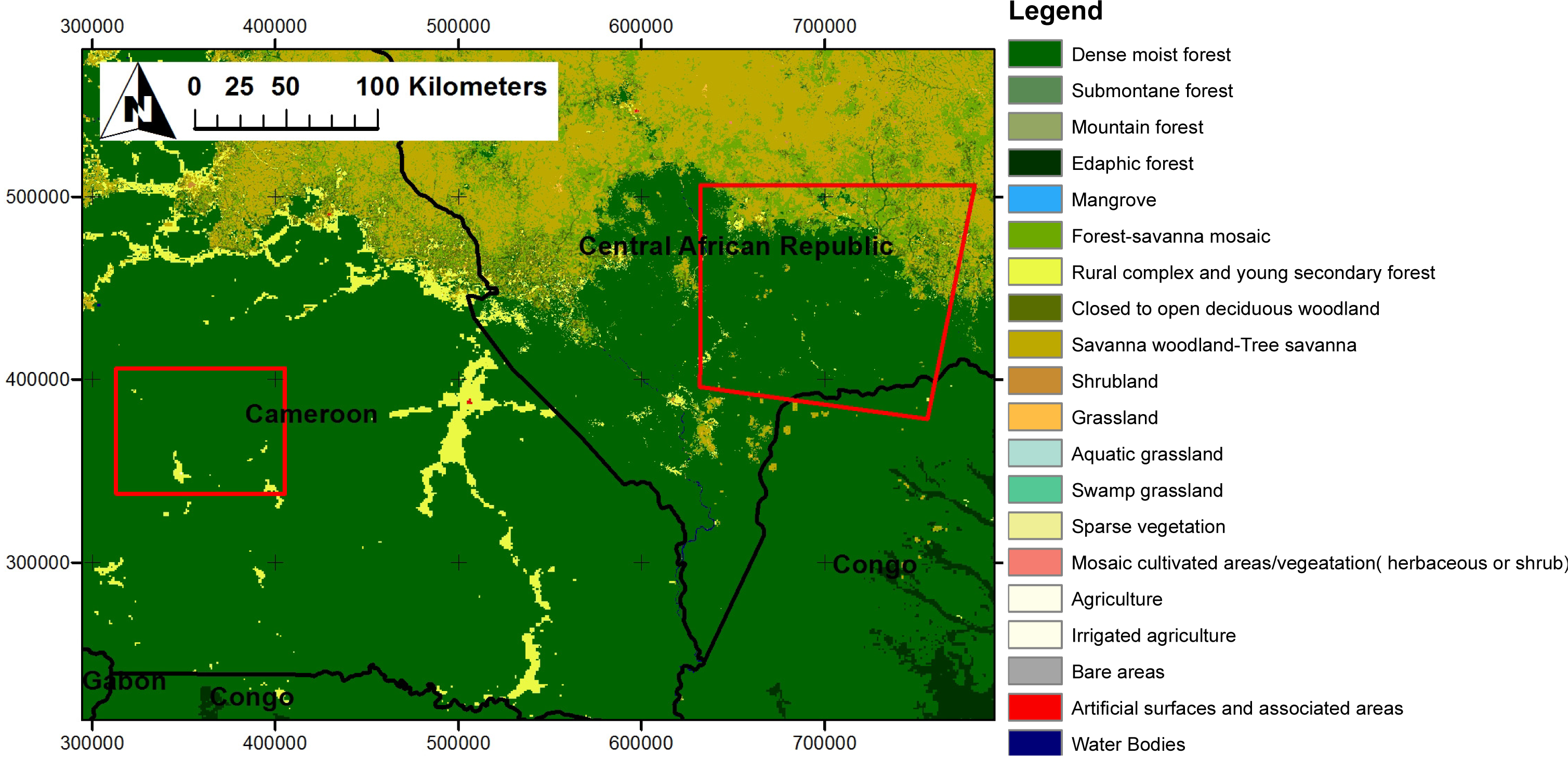
3. Data and Study Sites

Our approach to mapping forest degradation based on time series data was tested in two tropical countries in the Congo Basin within the project REDDAf (Reducing Emissions from Deforestation and Degradation in Africa, EC FP7) [28]. The first study site is located in Cameroon. For this study site, all the methodological developments, training, and also the derivation of the typical spectral behavior were done. The second study site is located in the Central African Republic, where the methods developed in Cameroon have been applied. The Cameroon site is characterized by dense moist forest, while the Central African Republic study site is partly situated in the transition zone to savanna woodland. The location of the two study sites is shown in Figure 1.
The first study site comprises the hilly terrain in the Eastern Province of Cameroon, where selective logging is performed by a certified concessionaire. The area of the study site is 6,356 km2. According to the world forestry atlas [39], more than half of the area is allocated to concessions, which means these areas are typically subject to selective logging. Four VHR (Very High Resolution, i.e., pixel size of 1 m or less) image subsets were ordered for training and verification.
The second study site covers 16,702 km2 and is located in the Central African Republic (CAR). It shows degradation patterns, mainly in the southern part (dense humid forest). The area is mostly flat. For the time series, Landsat data was used. For Cameroon, a period of twelve years was analysed (2000–2012). The data for CAR covers the epoch from 2001 to 2011. For training and accuracy assessment purposes, in Cameroon, four VHR sub-scenes were acquired. For CAR, also four, but smaller, VHR image subsets are available, in this case only used for accuracy assessment. A summary of the data sets used in this study is given in Table 1.

4. Methods

The overall process is illustrated in Figure 2. The individual processing steps are explained in Sections 4.1 and 4.2; the results are described in Section 5.

4.1. Data Preprocessing and Feature Selection

Necessary pre-processing steps include geometric and radiometric adjustment. Clearly, both geometric and radiometric congruence are needed if the spectral behavior over time is to be analyzed. In this study, only Landsat data is used to build the time series; therefore, no geometric adjustment was necessary between the Landsat scenes, as these data sets are already well-registered. However, in order to analyze the suitability of different features in comparison with ground truth data obtained from VHR data, an adjustment of the VHR images to the Landsat data was performed. This was done using tie points and an affine transformation. For radiometric calibration of all multi-temporal Landsat images, one image of the stack was selected as the master image. This master image should have the following properties: (1) free of haze; (2) mostly cloud-free; (3) and, in terms of image acquisition, close to the VHR image (if available). In Table 1, the master image for each of the study sites is printed in bold. All other images were adjusted relative to this master image using the radiometric adjustment procedure developed in the GSE FM REDD (GMES (Global Monitoring for the Environment and Security) Service Element on Forest Monitoring for REDD) project [41]. The method is based on pseudo-invariant features (PIFs); the details can be found in [42].
The aim of the next processing step is to select the best suitable feature for classification of the time series data. This was done for the Cameroon study site only. To this end, features, which have been found useful in the literature, were generated from the Landsat data. Features in this context are defined as pixel-based information, e.g., the original bands’ gray values, as well as derived values, such as vegetation indices. The list of features is given in Table 2. In order to select the best feature, all features were correlated to the reference data from VHR image interpretation (see Figure 3a). The features from the Landsat scene from 17 December 2010, were used for this analysis, as this data set was acquired at nearly the same time as the VHR image used for interpretation (2 December 2010). The result of this step is an analysis of the features’ suitability to map areas of selective logging by their correlation coefficient with the VHR interpretation result (see Table 2 in Section 5.1). In order to avoid residual geometric differences and to reduce noise, the reference data were aggregated to 90 × 90 m cells. Only those cells were used which carry valid data in the Landsat image (no stripes due to scan line corrector (SLC) failure) and are fully interpretable in the VHR image (no clouds). A subset of the raster with percentage of gap is shown in Figure 3b and resulted in 1,589 squares available for correlation all over the VHR image.

4.2. Multi-Temporal Classification

Based on the visual interpretation of VHR images, the temporal behavior of degradation areas (with varying intensity of degradation), as well as of intact forests, were extracted. The results of this interpretation and extraction process are detailed in Section 5.2. For these identified degradation areas, the spectral behavior was obtained from Landsat time-series data in the Cameroon study site. These real behavior curves were then grouped into typical behavior curves for three different degradation classes: strong degradation, weak degradation, and permanent degradation. In addition, areas of intact forest were also interpreted from the VHR image and based on that interpretation; three different types of intact forest were identified. All these six typical behavior curves were used as training data. This is a similar approach as used by [37] with the main difference that they had a much denser time series to build on. This dense time series allows the adjustment of the fit, which was not possible in our case with only one image per year. We had two reasons for using annual data only: first, in tropical areas, the phenology can usually be neglected and second, cloud cover is usually high preventing the acquisition of many usable images per year. In contrast to using training curves for classification, a decision tree model can also be employed, as was done by [36] classify forest disturbances.
Figure 4 illustrates the classification concept exemplarily for class “strong degradation” and a simplified annual update only. This figure is a schematic illustration and does not contain real data. The x-axis in Figure 4 shows the timeline with Tx being the acquisition date of the first image and theoretical annually repeated image acquisition. In reality, there are of course shorter and longer time intervals between the image acquisition dates. The y-axis shows the spectral response, which can be a single band, an index or whatever feature is selected (in our case soil fraction, see Section 5.2). In order to keep Figure 4 generally valid, no units are given for the y-axis. The colored lines at the top show a typical behavior curve for class “strong degradation” at each image acquisition point in time. For the classification, the behavior of each pixel in the time series data (example: black line at the bottom of Figure 4) is compared to these typical behavior curves and the residuals in terms of least squares are calculated to each of the typical behavior curves. Based on the minimal residuals, each pixel is classified to one point in time. The classification is performed using a minimum distance classifier. The class which shows the smallest difference to the given typical curves at each image acquisition point in time (best fitting curve) is assigned. The example pixel in Figure 4 shows the best fit (minimum spectral distance) with the typical curve at the time Tx+14 and is, therefore, assigned to this class. The method is working exactly as if there was an image with y bands, y being the number of image acquisition points in time available.
An additional dimension is added to the classification, as there is not only the class “strong degradation”, but five other classes: two more degradation classes and three intact forest classes. For each of them, the minimum distance has to be calculated for each image acquisition point in time. In our Cameroon study site with 12 available images, this added up to a sum of 72 classes (6 × 12). In a post-classification step, the classes were recorded to “degraded” and “non-degraded” for each image acquisition point in time leading to 24 classes. All pixels classified as “degraded” were then used as initial indicator pixels for each image acquisition point in time. In a next step, a context-analysis was performed. The roads and waterways were digitized and buffered by 1 km and non-forest areas, such as settlements, were buffered by 3 km. These distances were obtained from VHR data by analyzing the largest distance between a visible degradation feature (e.g., a gap) and the nearest logging road. Only pixels lying within these buffers were kept as indicator pixels. Finally, aggregation of the indicator pixels to larger areas was applied to facilitate linking of the “activity data” to emission factors. The aggregation procedure is based on the ArcGIS aggregation tool “Aggregate”. The specific parameters were set individually for Cameroon and CAR, as different logging practices are used. In Cameroon, a minimum mapping unit of 5 ha and an aggregation distance of 300 m was applied. The aggregation distance means that all indicator pixels with a maximum distance of 300 m between them were aggregated to larger areas. The minimum mapping unit determines, that only those areas were kept, which are above the minimum size of 5 ha. Equally, remaining holes were only retained if they were larger than 5 ha. For CAR, the aggregation distance had to be adjusted due to different logging practices and based on visual interpretation of the imagery was set to 800 m. The minimum mapping unit was kept the same as in Cameroon, i.e., 5 ha. Aggregation was performed iteratively: starting with the detections from the first image acquisition point in time, the aggregated result was then combined with the detections from the next image acquisition point in time and again an aggregation was performed. This is necessary as roads are often built in one year, but logging activity might only take place in the following years. Compared to work done in temperate forests, where, e.g., a forest disturbance is only classified as such if it there are at least three consecutive years with a difference above a specific threshold [38], such an approach was not possible in our tropical study areas, as the disturbance is often already lost after two or three years due to fast re-growth.

5. Results and Discussion

This section is divided into three parts: first, the results of the feature selection process; second, findings in terms of temporal spectral behavior after the logging event; and third, the final multi-temporal classification results including accuracy assessment for both study sites.

5.1. Feature Selection Results

The feature selection results are shown in Table 2. The highest correlation was achieved with SMA soil fraction leading to an R2 of 0.56, followed by the NDII7 and the TVI. In contrast to the literature [18], the use of SAVI instead of NDVI did not improve the correlation coefficient: both showed the same correlation coefficient of 0.47. The GEMI did not show any correlation with gaps, although it has been mentioned to be well suitable in the Amazon region [18]. The reason might be that this indicator is more sensitive to detecting re-vegetation than bare soil. In addition, the indicator mNDFI was calculated [25] but did not show a high correlation. In accordance with the literature, the TVI, NDII7, and SMA soil fraction features performed well in our analysis (compare Table 2). Our previous studies in the neighboring Republic of Congo (RoC) led to a similar ranking of features, although with generally higher R2 values (best result SMA soil fraction to gaps: 0.62). The reason for the lower correlation coefficients in Cameroon compared to the investigation performed in RoC can be found in the comparably smaller patterns of degradation in this certified logging concession. Based on these results, the SMA fraction soil was used in the multi-temporal classification.

5.2. Typical Temporal Curves of Degradation Patterns

The second result of this study is an improved understanding of the temporal behavior of the degradation areas after logging activities. For this purpose, all VHR images in Cameroon were interpreted and the mean soil fraction value for degradation patches over time were plotted (Figure 5). In order to complement the current findings, some results from our previous work in RoC are given here, as the results have not yet been published. In RoC, we found that the degradation signal (soil fraction) is lost within three to four years. Further, re-vegetation can be detected within the green vegetation fraction for longer time periods after the logging event. Immediately after the logging event, re-vegetation is sparse and therefore shows low GV fraction. After this initial re-vegetation period, approximately 2–10 years after the logging event, the GV fraction has been observed to be significantly above the average percentage of GV for intact forest.
In the Cameroon study site, with its smaller structured degradation patterns, the soil fraction signals are not as persistent over time as has been observed in RoC. Using the three VHR reference data sets together, complemented by the degradation areas selected from Landsat data in the very beginning of the time series, it can be seen that the elevated soil fraction is only visible for about two years in the Landsat time series (Figure 5). After that, the signal becomes blurred and reliable classification does not seem possible anymore, based solely on the soil fraction image (see Figure 5). Similar time frames have already been found in many studies in Latin America [43,44].
With regard to the behavior of the GV fraction, the same peak was found in the Cameroon study site as in RoC, but only after five years compared to about two to three years in RoC. These observations show that apparently re-vegetation has in general a clear peak after degradation activities, but the time of occurrence varies with logging practice or forest types. In the current classification scheme, the GV fraction is not yet integrated, as annual image coverage is available.

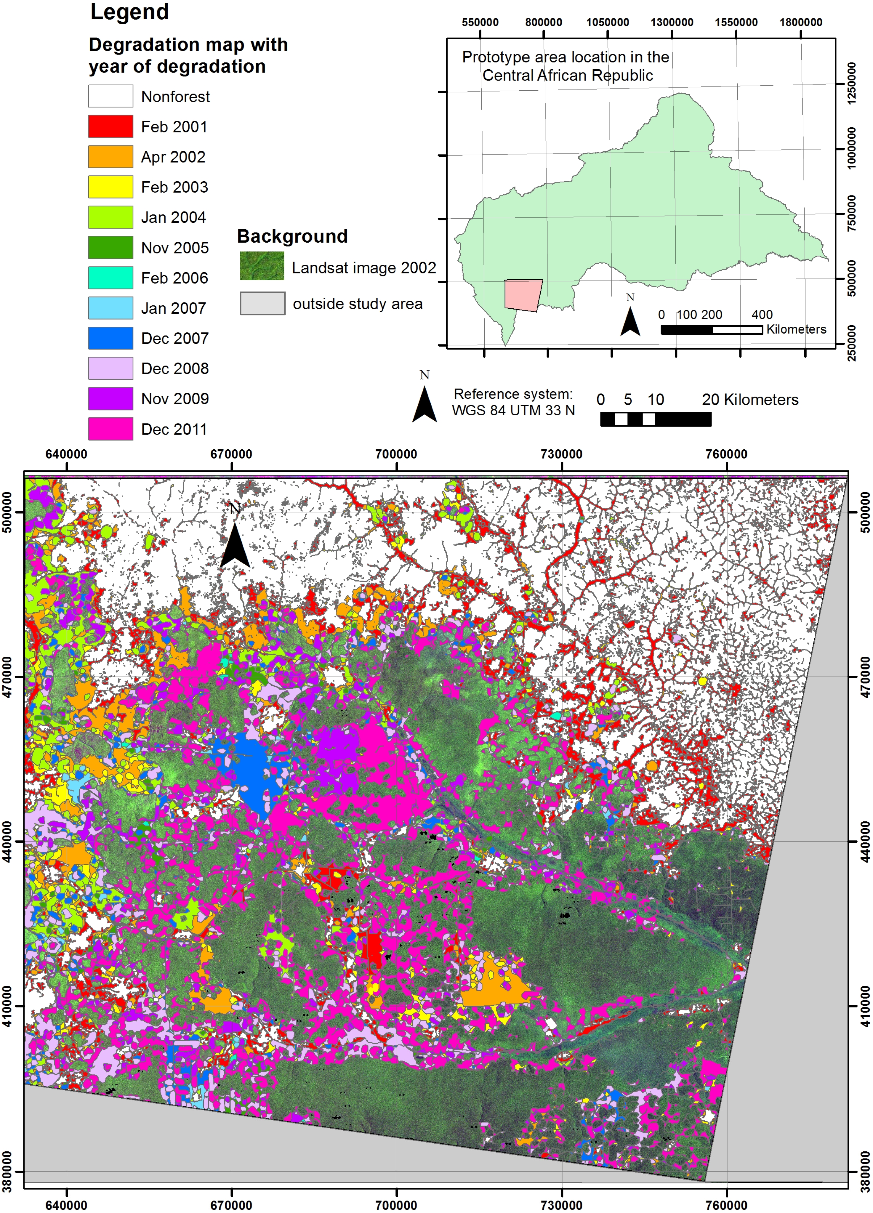
5.3. Results of Multi-Temporal Classification

Following the classification method described in Section 4.2, both test areas were classified into undegraded and degraded forest. Nonforest areas were masked out, the forest—nonforest classification was done by other consortium partners in the REDDAf project (methods and results given in [45]). The mapping result for the whole CAR study site is given in Figure 6; a detailed view is shown in Figure 7, where the typical selective logging pattern is visible in the Landsat image (left) and the resulting degradation map is shown on the right side. Accuracy of this result was assessed by means of systematic sampling in the areas, where VHR data is available. For each of the VHR image subsets, a regular grid of sampling points was generated. To calculate the number of sampling points respectively, the sampling distance for the regular grid, the following formula [46] was applied:
n h = p h ( 1 p h ) σ h 2
where nh is the number of samples per class; ph is estimated error rate; σh is accepted absolute standard error.
With an estimated error rate of 25% and an accepted absolute standard error of 2.5%, the minimum number of samples per class is 300 (and for both classes the total minimum number of sampling points is n = 600). In Cameroon, with a larger area covered by VHR data, more than 1,000 sample points could be interpreted. In CAR, the minimum number of sampling points was achieved, although large parts of the area covered by VHR data were located in the non-forest area. This is because, in CAR, the VHR image subsets were initially ordered for the accuracy assessment of a forest map.
Two different problems had to be taken into account in the visual interpretation of the sampling points: (a) the geometric accuracy and (b) the acquisition data of the VHR data. With regard to the first issue, a buffer of approximately 30 m (one Landsat pixel) was used to assess the degradation, i.e., if there is degradation visible within this buffer around the sample point in the VHR data, the sample point is labeled as “degraded”. For the proper validation of the results one has to consider that the acquisition date of the VHR image plays a decisive role and this aspect has to be taken into account. The time difference between the VHR scene and input image (Landsat) could create a false validation; for example, the sample points from the VHR image of 4 March 2010, in CAR only show the degradation up to this point in time (i.e., last Landsat observation before that time is 30 November 2009). Thus, the validator can only validate the degradation map up to this time. If degradation mapping results are integrated from after this time, some points might falsely appear as commission error, because even though the map is correct the degradation has taken place after the acquisition date of the VHR image.
In both study sites, the results show a very good overall accuracy of more than 87% (see Tables 3 and 4). The similar accuracy values are even more remarkable given that the system was developed in Cameroon and transferred to CAR. This proves the applicability and transferability of the developed system. The commission error (user’s accuracy of class “degradation”) is the main source of error. Two reasons could be identified for this error: (a) occurrence of swamp forest and (b) natural variances in the forest canopy. Swamp forests show—depending on the water level and/or season—varying spectral properties, which can be mistaken as degradation indicators. Due to the context analysis, which also includes waterways as possible routes for timber transport, these indicator pixels are kept and therefore wrongly included in the degradation map. In the verification areas in CAR, 46 sample points (7.6%) are located in swamp forest areas and most of them (37) are wrongly classified as degradation. In addition, natural variations in the spectral reflectance of the canopy, such as insect infestations, funghii, or the simple coincidence of a cluster of trees being temporarily leafless at the same time can also lead to minor commission errors.
This study is focused on forest degradation due to selective logging, as selective logging is the primary degradation driver in the given study sites. It is possible that degradation due to shifting cultivation might also have been detected to a minor extent in the frame of the classification process. There is a clear difference of our approach to common deforestation mapping, as most of the degradation areas still fall in the forest class according to most of the common forest definitions (minimum mapping unit, minimum crown cover, etc.) Exceptions to this rule are probably new big roads and large logging decks, which can be considered as deforestation.
In comparison to global attempts such as [5], the results of this study are much more detailed, both in terms of spatial detail (MMU), as well as in terms of thematic detail because the time of degradation is taken into account. A comparison with the intact forest land map (IFL) from [5] is shown in Figure 8. The black hatch shows the IFL areas according to [5], the colored patches are the detected degradation areas classified in this study. Aside from the spatial and thematic differences, there is also a difference in the time of data validity, which can be seen in the figure: most of the degradation detected by our approach for the year 2000 (red color) are also outside the IFL, which is based on imagery from 1990 and 2000. This means, the IFL map covers all forest landscapes, which still have been intact in 2000. More recent degradation appears in areas which still have been classified as IFL in 2000. A good agreement between both maps can be found in the south-western corner, where both IFL and our approach did not detect signs of degradation. The comparison in the CAR study site shows a similar result.
When the current results of the Cameroon study site are compared with the results of the 3D analysis based on Cosmo SkyMed (CSK) data [12], there is again a large difference in spatial detail. As with the VHR CSK data and the 3D approach, much smaller disturbances could be detected, but only for one point in time. In terms of operational applicability and costs, currently, the CSK data is still very expensive and has a small footprint. This means many CSK scenes would be needed to cover larger areas and, thus, our approach is currently the more economical alternative. On the other hand, the main drawback using optical data in the tropics is the risk of clouds and haze preventing the acquisition of high-quality imagery which is needed in our approach.

6. Conclusions and Outlook

The method presented in this study has been tested for mapping areas affected by selective logging in the Congo Basin. The method classifies time series data with annual coverage by applying typical curves of spectral behavior after logging events. These typical spectral curves have been obtained from visual interpretation of VHR imagery. The pixel-based results of this multi-temporal classification are then refined by context analysis and aggregated to larger areas of degradation. The results show similar outcomes in both the Cameroon and CAR study sites with overall accuracies around 87%. The main source of error is the commission error of degraded forest, i.e., natural variations in the spectral behavior of the canopy are mistaken as signals for degradation. For operational projects in the frame of REDD, knowledge of the extent to which forests have been degraded is crucial, as the carbon content is typically much lower than for pristine (undisturbed) forest. In comparison with an existing global map of intact forest land, there are the obvious differences in spatial detail due to different minimum mapping units and the time of data acquisition, but, generally, there is a good agreement.
Further work will include the test of transfer to other regions, the integration of different, possibly higher-resolution data sets and the integration of the GV fraction as an indicator for re-vegetation, especially if an annual coverage is not feasible. The final processing step will be the integration of this activity data map with emission factors to achieve carbon estimates, estimates which are ultimately required in the REDD reporting.

Acknowledgments

The research leading to these results has received funding from the European Union’s Seventh Framework Programme under grant agreement n°262775 (REDDAf project). Preparatory work and the analysis done in the Republic of Congo mentioned in this paper have been funded by the European Space Agency under the project “GMES Service Elements for Forest Monitoring—Extensions for REDD”. The authors would like to thank the anonymous reviewers for their valuable comments and suggestions, which helped to greatly improve the previous version of this paper.

Conflicts of Interest

The authors declare no conflict of interest.

References

  1. Nepstad, D.C.; Verissimo, A.; Alencar, A.; Nobre, C.; Lima, E.; Lefebvre, P.; Schlesinger, P.; Potter, C.; Moutinho, P.; Mendoza, E. Large-scale impoverishment of Amazonian forests by logging and fire. Nature 1999, 398, 505–508. [Google Scholar]
  2. Collomb, J.-G.; Mikissa, J.-B.; Minnemeyer, S.; Mundunga, S.; Nzao, N.H.; Madouma, J.; de Mapaga, J.D.; Mikolo, C.; Rabenkogo, N.; Akagah, S.; et al. First look at logging in Gabon. Available online: http://www.globalforestwatch.org/common/gabon/english/report.pdf (accessed on 24 April 2012).
  3. Cochrane, M.A.; Skole, D.L.; Matricardi, E.A.T.; Barber, C.; Chomentowski, W. Selective Logging, Forest Fragmentation and Fire Disturbance: Implications of Interaction and Synergy for Conservation. In Working Forests in the Neotropics: Conservation through Sustainable Management; Columbia University Press: New York, NY, USA, 2004; pp. 301–324. [Google Scholar]
  4. Nasi, R.; VanVliet, N. Case Studies on Measuring and Assessing Forest Degradation: Defaunation and Forest Degradation in Central African Logging Concession: How to Measure the Impacts of Bushmeat Hunting on the Ecosystem. Available online: http://www.fao.org/docrep/012/k7178e/k7178e00.pdf (accessed on 21 December 2013).
  5. Potapov, P.; Yaroshenko, A.; Turubanova, S.; Dubinin, M.; Laestadius, L.; Thies, C.; Aksenov, D.; Egorov, A.; Yesipova, Y.; Glushkov, I.; et al. Mapping the world’s intact forest landscapes by remote sensing. Ecol. Soc 2008, 13, 51. [Google Scholar]
  6. FAO. Forests and Climate Change Working Paper. Available online: http://www.fao.org/docrep/009/j9345e/j9345e08.htm (accessed on 21 December 2013).
  7. GOFC-GOLD (Global Observation of Forest and Land Cover Dynamics). A Sourcebook of Methods and Procedures for Monitoring and Reporting Anthropogenic Greenhouse Gas Emissions and Removals Associated with Deforestation, Gains and Losses of Carbon Stocks in Forests Remaining Forests, and Forestation; GOFC-GOLD Land Cover Project Office, Wageningen University: Wageningen, The Netherlands, 2012. [Google Scholar]
  8. Stone, T.A.; Lefebvre, P. Using multi-temporal satellite data to evaluate selective logging in Para, Brazil. Int. J. Remote Sens 1998, 19, 2517–2526. [Google Scholar]
  9. Duveiller, G.; Defourny, P.; Desclée, B.; Mayaux, P. Deforestation in central africa: Estimates at regional, national and landscape levels by advanced processing of systematically-distributed landsat extracts. Remote Sens. Environ 2008, 112, 1969–1981. [Google Scholar]
  10. Laporte, N.T.; Stabach, J.A.; Grosch, R.; Lin, T.S.; Goetz, S.J. Expansion of industrial logging in Central Africa—Supporting online material. Science 2007. [Google Scholar] [CrossRef]
  11. de Wasseige, C.; Defourny, P. Remote sensing of selective logging impact for tropical forest management. For. Ecol. Manag 2004, 188, 161–173. [Google Scholar]
  12. Deutscher, J.; Perko, R.; Gutjahr, K.; Hirschmugl, M.; Schardt, M. Mapping tropical rainforest canopy disturbances in 3D by COSMO-SkyMed spotlight InSAR-Stereo data to detect areas of forest degradation. Remote Sens 2013, 5, 648–663. [Google Scholar]
  13. Asner, G.P.; Knapp, D.E.; Cooper, A.N.; Bustamente, M.M.C.; Olander, L.P. Ecosystem structure throughout the Brazilian Amazon from Landsat observations and automated spectral unmixing. Earth Interact 2005, 9, 1–31. [Google Scholar]
  14. Souza, C.M.; Roberts, D.A.; Cochrane, M.A. Combining spectral and spatial information to map canopy damage from selective logging and forest fires. Remote Sens. Environ 2005, 98, 329–343. [Google Scholar]
  15. Asner, G.P.; Keller, M.; Pereira, R.; Zweede, J.C. Remote sensing of selective logging in Amazonia assessing limitations based on detailed field observations, Landsat ETM+, and textural analysis. Remote Sens. Environ 2002, 80, 483–496. [Google Scholar]
  16. Souza, C.M.; Roberts, D.A.; Monteiro, A.L. Multitemporal analysis of degraded forests in the Southern Brazilian Amazon. Earth Interact 2005, 9, 1–25. [Google Scholar]
  17. Jackson, R.D.; Huete, A.R. Interpreting vegetation indices. Prev. Vet. Med 1991, 11, 185–200. [Google Scholar]
  18. Asner, G.P.; Hicke, J.A.; Lobell, D.B. Per-Pixel Analysis of Forest Structure: Vegetation Indices, Spectral Mixture Analysis and Canopy Reflectance Modeling. In Remote Sensing of Forest Environments: Concepts and Case Studies; Springer: New York, NY, USA, 2003; pp. 209–254. [Google Scholar]
  19. Al Mohamed, I. Erfassung und Bewertung von degradierten Böden mit Fernerkundung und GIS in Nordwest-Syrien. Technical University of Dresden, Dresden, Germany, 2011. [Google Scholar]
  20. Matricardi, E.A.T.; Skole, D.L.; Pedlowski, M.A.; Chomentowski, W.; Fernandes, L.C. Assessment of tropical forest degradation by selective logging and fire using landsat imagery. Remote Sens. Environ 2010, 114, 1117–1129. [Google Scholar]
  21. Thenkabail, P.S.; Enclona, E.A.; Ashton, M.S.; Legg, C.; de Dieu, M.J. Hyperion IKONOS, ALI, and ETM+ sensors in the study of African rainforests. Remote Sens. Environ 2004, 90, 23–43. [Google Scholar]
  22. Ponzoni, F.J.; Galvao, L.S.; Liesenberg, V.; Santos, J.R. Impact of multi-angular CHRIS/PROBA data on their empirical relationships with tropical forest biomass. Int. J. Remote Sens 2010, 31, 5257–5273. [Google Scholar]
  23. Souza, C.; Barreto, P. An alternative approach for detecting and monitoring selectively logged forests in the Amazon. Int. J. Remote Sens 2000, 21, 173–179. [Google Scholar]
  24. Asner, G.P. The Carnegie Landsat Analysis System (Version 1.0 21); Asner Lab: Stanford, CA, USA, 2005. [Google Scholar]
  25. Haas, S. Monitoring Forest Degradation for Redd in Cameroon. University of Karlsruhe, Karlsruhe, Germany, 2009. [Google Scholar]
  26. Sanderson, E.W.; Jaiteh, M.; Levy, M.A.; Redford, K.H.; Wannebo, A.V.; Woolmer, G. The human footprint and the last of the wild. BioScience 2002, 52, 891–904. [Google Scholar]
  27. Bontemps, S.; Langner, A.; Defourny, P. Monitoring forest changes in borneo on a yearly basis by an object-based change detection algorithm using spot-vegetation time series. Int. J. Remote Sens 2012, 33, 4673–4699. [Google Scholar]
  28. Verbesselt, J.; Zeileis, A.; Herold, M. Near real-time disturbance detection using satellite image time series: Drought detection in Somalia. Remote Sens. Environ 2012, 123, 98–108. [Google Scholar]
  29. Koltunov, A.; Ustin, S.L.; Asner, G.P.; Fung, I. Selective logging changes forest phenology in the Brazilian Amazon: Evidence from MODIS image time series analysis. Remote Sens. Environ 2009, 113, 2431–2440. [Google Scholar]
  30. Eklundh, L.; Johansson, T.; Solberg, S. Mapping insect defoliation in Scots pine with MODIS time-series data. Remote Sens. Environ 2009, 113, 1566–1573. [Google Scholar]
  31. Jin, S.; Sader, S.A. MODIS time-series imagery for forest disturbance detection and quantification of patch size effects. Remote Sens. Environ 2005, 99, 462–470. [Google Scholar]
  32. Margono, B.A.; Turubanova, S.; Zhuravleva, I.; Potapov, P.; Tyukavina, A.; Baccini, A.; Goetz, S.; Hansen, M.C. Mapping and monitoring deforestation and forest degradation in sumatra (Indonesia) using Landsat time series data sets from 1990 to 2010. Environ. Res. Lett 2012, 7, 1–16. [Google Scholar]
  33. Healey, S.; Moisen, R.; Masek, J.; Cohen, W.; Goward, S.; Powell, S.; Nelson, M.; Jacobs, D.; Lister, A.; Kennedy, R.; et al. Measurement of Forest Disturbance and Regrowth with Landsat and Forest Inventory and Analysis Data: Anticipated Benefits from Forest and Inventory Analysis? Proceedings of the Seventh Annual Forest Inventory and Analysis Symposium, Portland, OR, USA, 3–6 October 2005; pp. 171–178.
  34. Kennedy, R.E.; Cohen, W.B.; Schroeder, T.A. Trajectory-based change detection for automated characterization of forest disturbance dynamics. Remote Sens. Environ 2007, 110, 370–386. [Google Scholar]
  35. Kennedy, R.E.; Yang, Z.; Cohen, W.B. Detecting trends in forest disturbance and recovery using yearly Landsat time series: 1. LandTrendr—Temporal segmentation algorithms. Remote Sens. Environ 2010, 114, 2897–2910. [Google Scholar]
  36. Huang, C.; Goward, S.N.; Masek, J.G.; Thomas, N.; Zhu, Z.; Vogelmann, J.E. An automated approach for reconstructing recent forest disturbance history using dense Landsat time series stacks. Remote Sens. Environ 2010, 114, 183–198. [Google Scholar]
  37. Brooks, E.B.; Wynne, R.H.; Thomas, V.A.; Blinn, C.E.; Coulston, J.W. On-the-fly massively multitemporal change detection using statistical quality control charts and landsat data. IEEE Trans. Geosci. Remote Sens 2013, 1–17. [Google Scholar]
  38. Zhu, Z.; Woodcock, C.E.; Olofsson, P. Continuous monitoring of forest disturbance using all available Landsat imagery. Remote Sens. Environ 2012, 122, 75–91. [Google Scholar]
  39. Mertens, B.; Steil, M.; Nsoyuni, L.A.; Shu, G.N.; Minnemeyer, S. Interactive Forestry Atlas of Cameroon (Version 2.0). http://www.wri.org/publication/interactive-forestry-atlas-cameroon-version-2-0 (accessed on 16 February 2009).
  40. Verhegghen, A.; Mayaux, P.; de Wasseige, C.; Defourny, P. Mapping Congo Basin vegetation types from 300 m and 1 km multi-sensor time series for carbon stocks and forest areas estimation. Biogeosciences 2012, 9, 5061–5079. [Google Scholar] [Green Version]
  41. GSE FM REDD (GMES Service Elements for Forest Monitoring—Extensions for REDD). Available online: http://www.redd-services.info/content/gse-fm-redd (accessed on 21 December 2013).
  42. Schmitt, U.; Deutscher, J. Integration to REDD Toolbox; GSE-REDD-TN1-RT-Ph2; Joanneum Research: Graz, Austria, 2012. [Google Scholar]
  43. Pereira, R.; Zweede, J.; Asner, G.P.; Keller, M. Forest canopy damage and recovery in reduced-impact and conventional selective logging in eastern Para, Brazil. For. Ecol. Manag 2002, 168, 77–89. [Google Scholar]
  44. Asner, G.P.; Keller, M.; Pereira, R.; Zweede, J.C.; Silva, J.N.M. Canopy damage and recovery after selective logging in Amazonia: Field and satellite studies. Ecol. Appl 2004, 14, 280–298. [Google Scholar]
  45. Fichet, L.; Sannier, C. Development of an Operational System for Monitoring Forest Cover at National Scale in 1990, 2000 and 2010. Proceedings of the XV Symposium SELPER, Cayenne, France, 19–23 November 2012.
  46. Bossard, M.; Feranec, J.; Otahel, J. CORINE Land Cover Technical Guide—Addedum 2000; European Environment Agency: Copenhagen, Denmark, 2000. [Google Scholar]
Figure 1. Location of the two study sites in Cameroon and Central African Republic with a Congo Basin vegetation types map as background [40]. The areas marked in red represent the study sites.
Remotesensing 06 00756f1
Figure 2. Overview of processing steps.
Remotesensing 06 00756f2
Figure 3. (a) Visual interpretation result; (b) 90 × 90 m aggregated visual interpretation result (percentage of gaps for interpretable areas) superimposed on Landsat SLC-off image (bands 432).
Remotesensing 06 00756f3
Figure 4. Schematically classification system for the multi-temporal stack of features (e.g., soil fraction). The soil fraction behavior of one example pixel (bottom: black line) is compared to typical behavior of degraded areas (top: colored lines) and classified to the best fitting line.
Remotesensing 06 00756f4
Figure 5. Performance of the temporal behavior of mean soil fraction values of degradation areas from different years in the Cameroon study site.
Remotesensing 06 00756f5
Figure 6. Final degradation map for CAR study site. The different colors indicate the time of (first) degradation occurrence.
Remotesensing 06 00756f6
Figure 7. Detail of CAR result: (left) Landsat image 2001, (right) Landsat image 2001 superimposed with nonforest areas (white) and forest areas affected by degradation (red).
Remotesensing 06 00756f7
Figure 8. Final degradation map for the Cameroon study site in comparison with the IFL map [5]. The different colors indicate the time of degradation occurrence mapped by our approach, the black hatched area represent the areas classified as IFL.
Remotesensing 06 00756f8
Table 1. Imagery used for the two study sites in Cameroon and Central African Republic (CAR).
SensorAcquisition DateExtentUsed for

Test Area Cameroon
Landsat ETM+5 December 20006,356 km2Time series mapping
Landsat ETM+25 January 2002
Landsat ETM+27 December 2002
Landsat SLC-off7 April 2005
Landsat SLC-off20 January 2006
Landsat SLC-off7 January 2007
Landsat SLC-off25 December 2007
Landsat SLC-off27 December 2008
Landsat SLC-off30 December 2009
Landsat SLC-off17 December 2010
Landsat SLC-off18 January 2011
Landsat SLC-off26 April 2012
Quickbird27 November 20076.2 × 5.7 kmTraining and accuracy assessment
Quickbird30 May 20088 × 11.2 km
Quickbird2 December 20105 × 5 km
Worldview-212 June 20128.5 × 11.7 km

Test Area CAR

Landsat ETM+9 February 200116,702 km2Time series mapping
Landsat ETM+1 April 2002
Landsat ETM+15 February 2003
Landsat SLC-off1 January 2004
Landsat SLC-off19 November 2005
Landsat SLC-off7 February 2006
Landsat SLC-off9 January 2007
Landsat SLC-off27 December 2007
Landsat SLC-off29 December 2008
Landsat SLC-off30 November 2009
Landsat SLC-off6 December 2011
Worldview6 January 20115 × 5 kmAccuracy assessment
Quickbird4 March 20105 × 5 km
Quickbird26 March 20115 × 5 km
Quickbird18 March 20115 × 3.5 km
Table 2. R2 values (all 90 m squares, n = 1,589) for percentage of gaps free of vegetation as obtained from the Very High Resolution (VHR) image (17 December 2010) in comparison to different features generated from Landsat (2 December 2010).
FeatureCorrelation Landsat—VHR 2010 (R2)
SMA 45 Soil fraction0.56
NDII7 (Normalized Difference Infrared Index with Landsat band 7)0.55
TVI (Transformed Vegetation Index)0.52
SAVI (Soil-Adjusted Vegetation Index)0.47
NDVI (Normalized Difference Vegetation Index)0.47
NDII5 (Normalized Difference Infrared Index with Landsat band 5)0.35
Band 3 (red)0.30
Band 5 (short wave infrared)0.19
Band 4 (near infrared)0.07
mNDFI (Modified Normalised Difference Fraction Index)0.05
RVI (Ratio-Vegetation Index)0.00
GEMI (Global Environment Monitoring Index)0.00
Table 3. Confusion matrix for Cameroon degradation map, 1,022 label points used.


Reference

Undegraded Forest
Degraded Forest
Total
User's Accuracy
ClassificationUndegraded forest6972572296.5%
Degraded forest10020030066.7%
Total7972251,022
Producer's accuracy87.5%88.9%Overall accuracy: 87.8%
Kappa coefficient: 0.68
Table 4. Confusion matrix for CAR degradation map, 603 label points used.


Reference

Undegraded Forest
Degraded Forest
Total
User's Accuracy
ClassificationUndegraded forest4212444594.6%
Degraded forest4411415872.2%
Total465138603
Producer's accuracy90.5%82.6%Overall accuracy: 88.7%
Kappa coefficient: 0.7

