Continuous Extraction of Subway Tunnel Cross Sections Based on Terrestrial Point Clouds

Abstract

An efficient method for the continuous extraction of subway tunnel cross sections using terrestrial point clouds is proposed. First, the continuous central axis of the tunnel is extracted using a 2D projection of the point cloud and curve fitting using the RANSAC (RANdom SAmple Consensus) algorithm, and the axis is optimized using a global extraction strategy based on segment-wise fitting. The cross-sectional planes, which are orthogonal to the central axis, are then determined for every interval. The cross-sectional points are extracted by intersecting straight lines that rotate orthogonally around the central axis within the cross-sectional plane with the tunnel point cloud. An interpolation algorithm based on quadric parametric surface fitting, using the BaySAC (Bayesian SAmpling Consensus) algorithm, is proposed to compute the cross-sectional point when it cannot be acquired directly from the tunnel points along the extraction direction of interest. Because the standard shape of the tunnel cross section is a circle, circle fitting is implemented using RANSAC to reduce the noise. The proposed approach is tested on terrestrial point clouds that cover a 150-m-long segment of a Shanghai subway tunnel, which were acquired using a LMS VZ-400 laser scanner. The results indicate that the proposed quadric parametric surface fitting using the optimized BaySAC achieves a higher overall fitting accuracy (0.9 mm) than the accuracy (1.6 mm) obtained by the plain RANSAC. The results also show that the proposed cross section extraction algorithm can achieve high accuracy (millimeter level, which was assessed by comparing the fitted radii with the designed radius of the cross section and comparing corresponding chord lengths in different cross sections) and high efficiency (less than 3 s/section on average).

1. Introduction

Because underground structures such as tunnels require routine inspections and maintenance for their optimal use, efficient and accurate tunnel inspections are necessary. The shape, width and area of the cross sections of constructed or natural tunnels can be used to determine their structural stability. These estimations are generally conducted based on sparsely sampled points that are surveyed using a total station. This approach requires a considerable amount of time and effort, although non-prism total stations are now available [1]. However, it is often difficult to survey and analyze the construction sites and tunnels that are currently in use. Many recent studies have discussed using digital photogrammetry to determine the internal cross sections of tunnels [1,2]. However, in many cases, it is difficult to discriminate the subjects using photography because of the restricted light sources in the poor environments and working conditions in tunnels, and it is difficult to capture the characteristics of irregular internal cross sections of tunnels.

The application of laser technology is rapidly expanding and offers decreased costs and increased accuracy. Therefore, 3D laser scanners make it possible to obtain high-accuracy data and high location precision, even under disadvantageous conditions. Tsakiri et al. [3] discussed several surface modeling methods that were implemented to monitor deformation and various approaches to measure deformation from the modeled surfaces. Using a weighted-constraint, least-squares curve-fitting approach, Gordon and Lichti [4] developed a modeling strategy from the fundamental beam-deflection equations to permit the usage of coarse-precision terrestrial laser scanner observations to accurately measure the vertical deflections of deforming beams. Gosliga et al. [5] and Lindenbergh et al. [6] described a workflow for terrestrial laser scanning to detect deformation by taking advantage of both data redundancy and the individual point quality. Schneider [7] applied an analysis of highly redundant unstructured point clouds that represent the surfaces of objects to monitor the bending line of a television tower. Monserrat and Crosetto [8] proposed a procedure to measure land deformation using repeated terrestrial laser scanning (TLS) acquisitions and the least-squares surface-matching algorithm proposed by Gruen and Akca [9]. Pejic' [10] presented a method for inspecting tunnel geometries that focused on the optimization of scan registrations, the georeferencing approach and the design of the survey control network.

A tunnel's internal cross section can be obtained from large quantities of laser scanning data of the tunnel, and precise outbreak and underbreak quantities can be calculated. Yoon et al. [11] developed a prototype of a laser-based tunnel scanning system to extract the installations and the physically damaged parts of a tunnel liner using the geometric and radiometric features of the scanning data. Gikas [12] explored the potential of laser scanning technology to accurately track excavation and construction activities of highway tunnels. A tunnel cross section management system was developed based on terrestrial laser scanning to determine arbitrary cross sections [13].

Two methods are commonly used to extract the cross sections of a tunnel from TLS data [12]. The first method extracts the cross sections from a 3D model of the tunnel tube that is generated from TLS data using NURBS [14], which uses standard geometric models such as a cylinder [5] or a 3D mesh model [3], to approximate a geometric domain. However, the reconstruction of the entire 3D model of a tunnel may involve processing millions of laser points, which predictably leads to large computation costs. The approximation of the fitted model to the real tunnel also degrades the accuracy of the cross section estimation. The second method determines the cross section based only on a subset of the point cloud, which forms a thin, sliced, solid body. In this case, the vertical plane that defines the cross section is determined in terms of the central axis of the tunnel, and the cross section is developed using a poly-line string that results from projecting the point-cloud data in the sliced body onto the plane of the desired cross section [15]. As an extension of our previous work [16], this paper proposes an algorithm to extract cross sections that determines the cross-sectional points using a different strategy.

First, the central axis of the subway tunnel is determined using a 2D projection of the tunnel point cloud and multiple model (e.g., straight line, transition curve and curve) fitting using a so-called statistical testing algorithm and the RANSAC (RANdom SAmple Consensus) algorithm. Because the extraction of the central axis by multiple model fitting may suffer from noise in the tunnel point data and bending of the tunnel, we propose a global extraction algorithm based on segment-wise fitting. Oude Elberink et al. [17] presented a similar strategy of rail track modeling that integrated piece-wise fitting by Markov Chain Monte Carlo (MCMC) sampling and global optimization using a Fourier series. In addition, an algorithm proposed by Han et al. [15] is employed to adjust the pseudo cross-sectional plane, whose direction is subject to the errors that are generated from the fitting processes and from the noise and the positioning errors of the laser scanner. The cross-sectional points are then produced by intersecting a radial rotating line about the central axis of the tunnel within a vertical plane with the tunnel points. Although they have a notably high spatial resolution (millimeter level), the terrestrial laser points remain discrete; thus, no laser point intersects with the radial, which implies that no cross-sectional point can be acquired. To address the spatial discontinuity of a scattered-point cloud, we propose an algorithm to compute the cross-sectional point in terms of quadric parametric surface fitting in the vicinity of the extraction position. Finally, because the standard shape of the subway tunnel of interest is a circle, the fitting of a circle is implemented using RANSAC to remove the irrelevant points and retain the real cross-sectional points so that the cross sections in the circular form are extracted.

We begin by describing the algorithm used to extract the central axis of a tunnel in Section 2. The next section introduces the algorithm for the continuous extraction of cross sections based on the extracted central axis from the terrestrial point clouds. Section 4 discusses the test results, after which we offer conclusions and suggestions for further research in Section 5.

2. Extraction of the Central Axis of a Tunnel

To extract so-called continuous (i.e., at any interval) cross sections from terrestrial point clouds, the central axis of the subway tunnel must be determined. The central axis can be used to determine the direction of a cross-sectional plane at any interval. Tunnels are generally tubular and can be simplified as narrow and relatively long 2D objects if they are projected onto horizontal or vertical planes. Many skeletonizing methods that are popular in the computer vision, medical visualization and feature representation fields are applicable for estimating the centerline of tubular objects [15,18–20]. Similar to the idea of the 2D projection, the 3D central axis of a tunnel is estimated in terms of the projections of the tunnel points on the XOY and the YOZ planes.

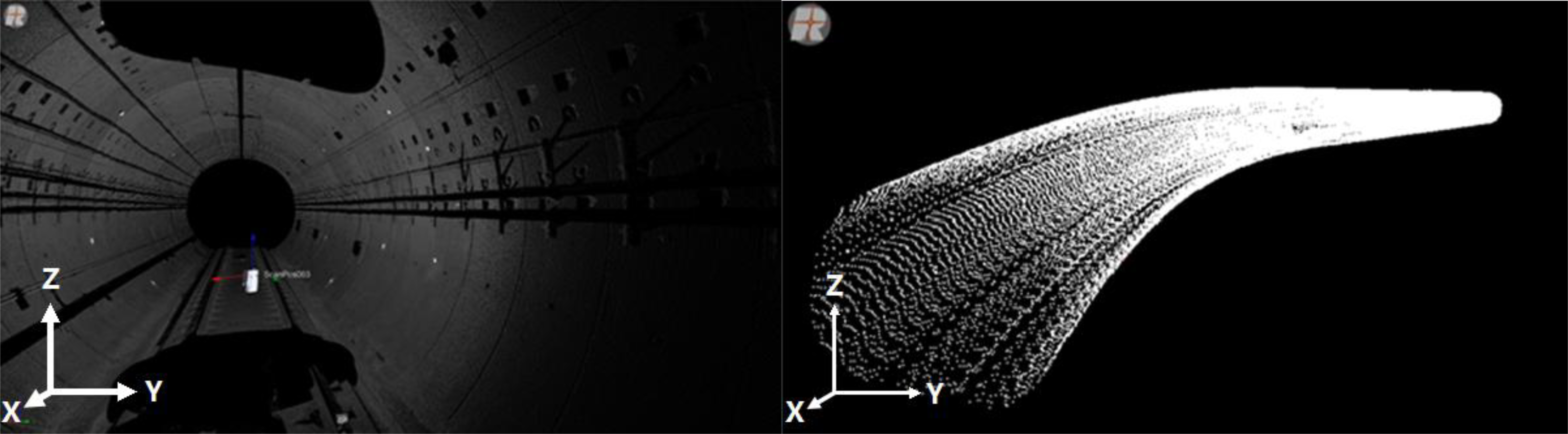
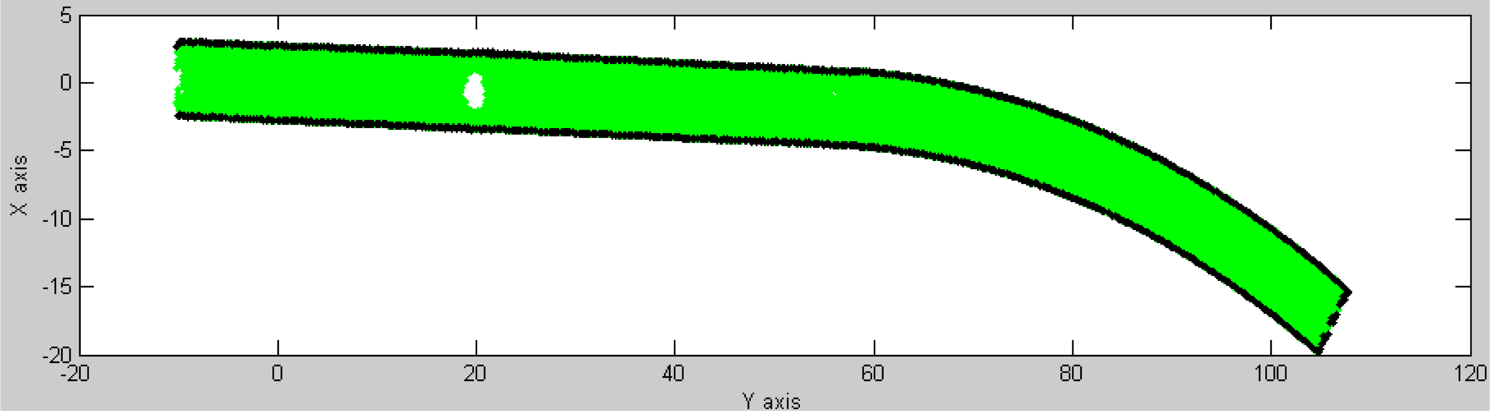
2.1. Determination of the Central Axis of a Tunnel Based on 2D Projection

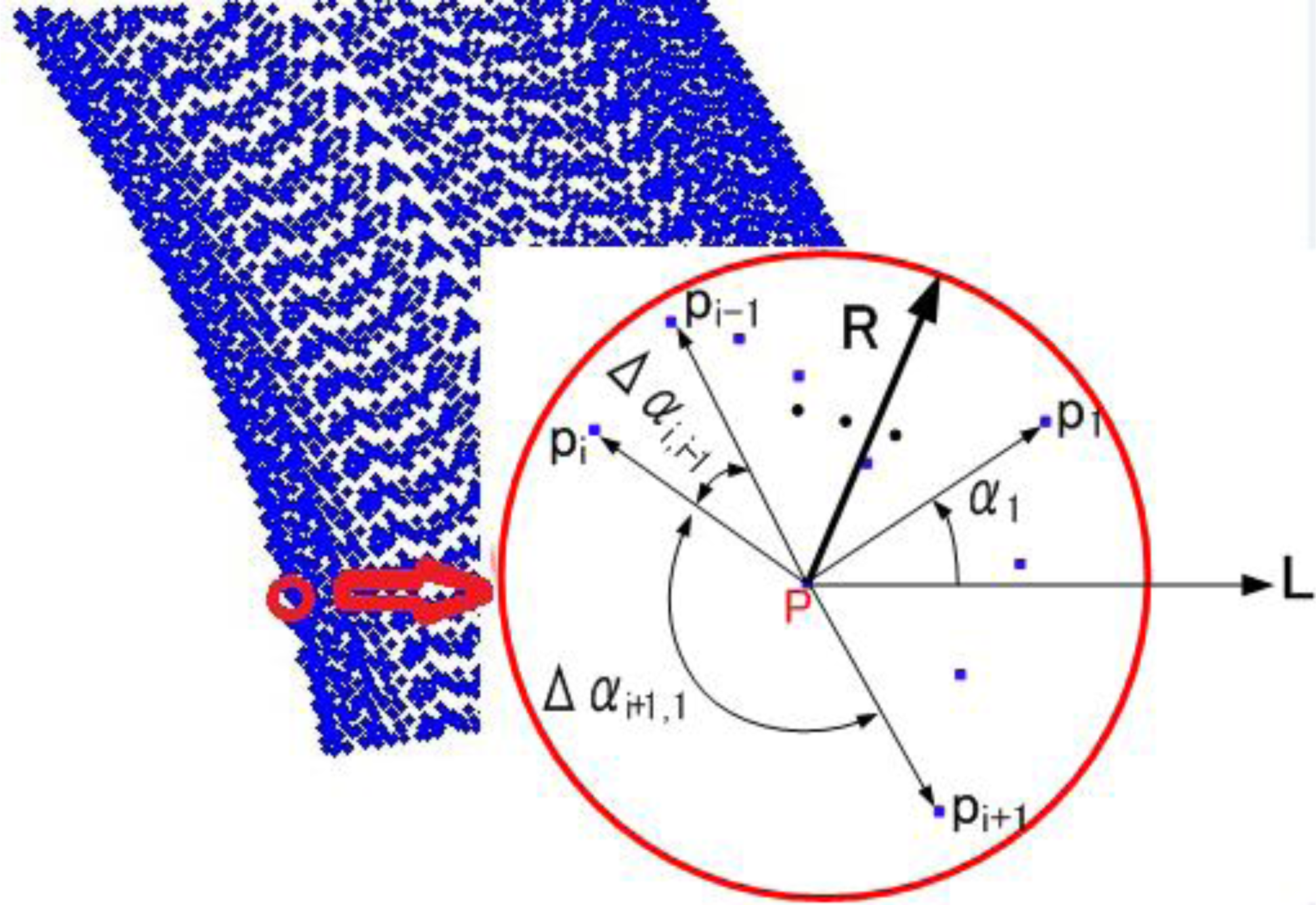
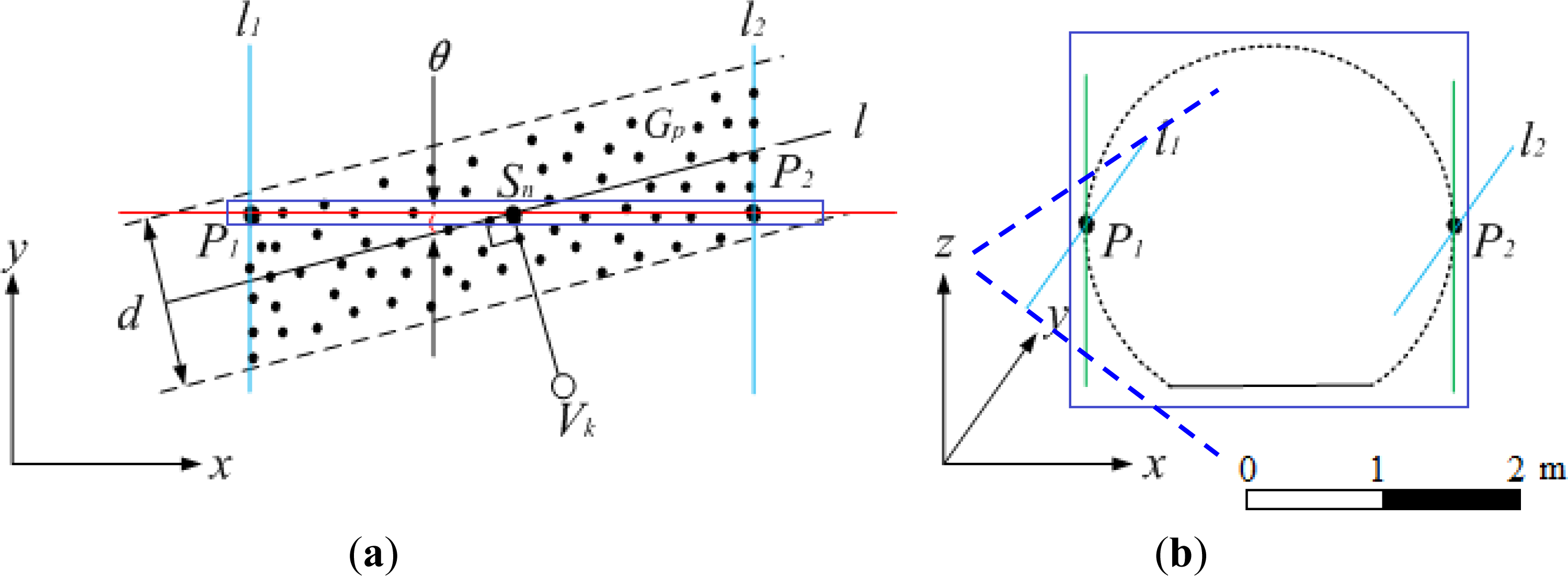
2.1.1. Estimation of the Boundary Points

The tunnel point clouds are projected onto the XOY plane, from which we extract the boundary points of both sides of the tunnel. An algorithm for boundary point extraction is proposed using a moving window. Figure 1 shows a circular window with a predefined radius that is centered at the point of interest P. All points within the window are considered the neighboring points of point P. The polar angles of the neighboring points are computed relative to point P (e.g., α₁). We then calculate the differences between consecutive polar angles. If point P is a boundary point, the difference Δα_{i + 1,i} between boundary points P_i and P_{i + 1} is much larger than the difference Δα_{i,i − 1} between boundary point P_i and interior point P_{i − 1}. Therefore, once the difference is greater than a predefined threshold, point P is labeled as a boundary point.

2.1.2. Fitting of the Bounding Lines

The bounding lines of a tunnel usually contain segments of straight lines, curves and transition curves, which are parameterized as follows:

• Straight line model:

  $$X=\mathit{aY}+b$$

  (1)
• Transition curve model:

  $$X={\mathit{cY}}^3+{\mathit{dY}}^2+\mathit{eY}+f$$

  (2)
• Curve model:

  $$X={\mathit{gY}}^2+\mathit{hY}+k$$

  (3)

where a and b are the parameters of a straight line; c, d, e, and f are the parameters of a transition curve; and g, h, and k are the parameters of a curve.

The bounding line fitting process includes the estimation of multiple models. To ensure the robustness of the fitting, the RANSAC algorithm [21] is used to estimate the parameters of the three models. Instead of using as much data as possible to obtain an initial solution and attempting to eliminate the invalid data points, RANSAC uses as small an initial data set as is feasible and enlarges this set using consistent data when possible. The RANSAC paradigm contains three unspecified parameters: (1) the error tolerance, which is used to determine whether a point is compatible with the model; (2) the number of subsets to attempt; and (3) the threshold t, which is the number of compatible points and is used to define that the correct model has been found. The determination of these three parameters is discussed in the introduction to RANSAC [21].

A statistical testing algorithm is proposed to automatically detect the initial models from the extracted boundary points so the proper model is selected to fit each segment of the bounding line. The statistical testing is implemented using straight-line, transition-curve and curve models.

The statistical testing process is implemented using a histogram, which illustrates the distribution of the discrete hypothesis model parameter sets that are computed during different iterations. The degree of convergence of a candidate parameter set is used as a criterion of the statistical testing. This criterion describes how the other sets converge to it and is calculated by dividing the number of converging sets by the total number of parameter sets. We construct vectors with two, four and three dimensions for each set of model parameters. The Euclidian distances between different vectors are computed to describe the deviation between the candidate parameter set and the other hypothesis model parameter sets. If the distance between a hypothesis set and the candidate set is smaller than the predefined threshold, the hypothesis set is considered the converging set of the candidate set, and the degree of convergence of the candidate set increases. In this method, the histogram of the candidate parameter sets is updated during each iteration using the newly calculated hypothesis parameter set. When the degree of convergence of a candidate parameter set reaches a predefined threshold, the candidate parameter set is detected as an initial model to fit the bounding line segment. If the degree of convergence fails to reach the threshold after a predefined number of iterations, we believe that there is no such model.

To visualize the statistical results, we illustrate them as a histogram (Figure 2). The horizontal axis denotes the mean value of the model parameters, and the vertical axis represents the degree of convergence of each cell. A high degree of convergence for a parameter reflects a high probability of finding the initial model.

After the initial model is detected, RANSAC is used to robustly estimate the optimized model parameters. Two, four, and three points are used to estimate the model parameters to fit a straight line, a transition curve and a curve, respectively. The criterion used to identify outliers is based on the deviations of the tested points from the fitted model. The inlier bounding points of a certain model are classified as a segment that is used in the following global optimization. The final optimal parameters are computed by the least-squares adjustment using the obtained inlier points.

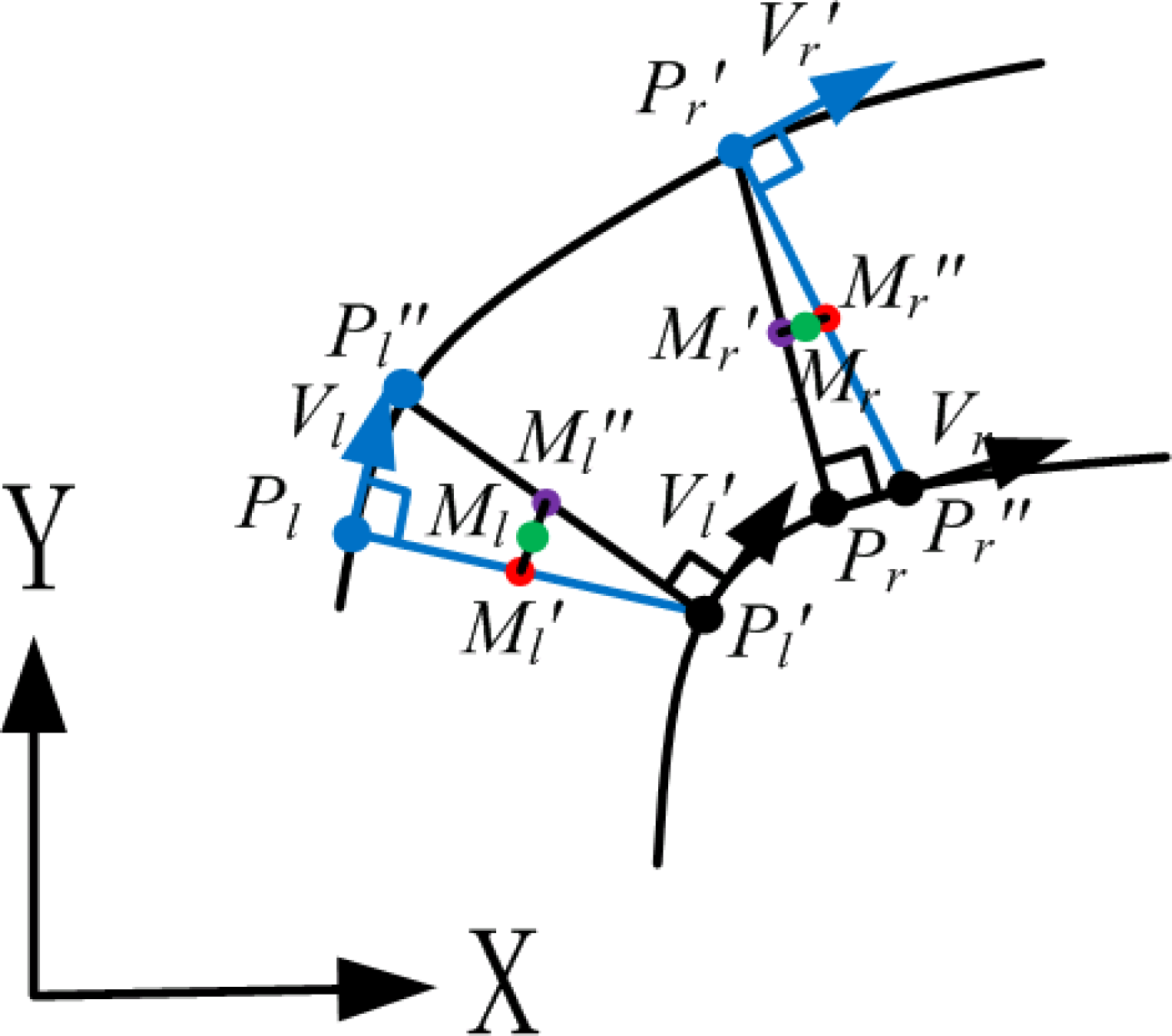
2.1.3. Fitting of the Central Axis

After fitting the bounding lines, the boundary points are evenly resampled. To extract the central axis of the tunnel, the normal vector V_l of the left bounding curve at boundary point P_l is determined (Figure 3). A straight line orthogonal to the normal vector reaches the right bounding curve from P_l and generates point P_l′. Theoretically, the radial line from point P_l′ that is orthogonal to V_l′ reaches the left bounding curve at point P_l, so the extracted central-axis point is the midpoint of the line P_l P_l′. However, because the bounding curves are subject to errors that are generated from the fitting processes, the radial orthogonal to V_l′ produces point P_l″ instead of point P_l. Figure 3 shows that M_l′ and M_l″ are the midpoints of P_l P_l′ and P_l′ P_l″, respectively. The extracted central-axis point is determined as M_l, which is the average of points M_l′ and M_l″. The same process is implemented from boundary point P_r on the right bounding curve to extract the point on the central axis as point M_r. Based on the extracted central-axis points, the presented strategy to fit a bounding line is used to generate the central axis. Because the extraction of the central axis is implemented on the XOY plane, the height of the central axis is determined as the average height of the tunnel points.

2.2. Global Adjustment of the Central Axis Using Segment-Wise Fitting

Because the extraction of the segments of the bounding lines and the central axis on the XOY plane using the three models may suffer from noise in the tunnel points, there may be deviations in the overlapping parts of adjacent fitted models (Figure 4). Therefore, we propose a global extraction algorithm to minimize the deviations.

To maintain consistency between adjacent fitted models, the divided segments overlap each other somewhat, and a global least-squares adjustment is developed to implement the multiple model fitting of all of the segments together by minimizing the deviations in the overlapping parts of adjacent fitted models. Using Equations (1)–(3), the constraints are derived between a straight line, a transition curve and a curve, respectively, and are added to the adjustment model. For example, Equation (4) parameterizes the constraint between a straight line and a transition curve:

$$a_{i}Y+b_i-(c_j{Y}^3+d_j{Y}^2+e_{j}Y+f_j)=0$$

(4)

where a_i and b_i are the line parameters of segment i, c_j, d_j, e_j, f_j are the transition curve parameters of segment j, and Y is the Y coordinate of a point in the overlap region between segments i and j.

Equation (4) describes the constraint that the X coordinates computed by any Y coordinate in the overlap region between segments i and j using the model parameters of segments i and j are theoretically equal.

The coefficient matrix of the observation and constraint equations of the global least-squares adjustment is derived in Equation (5):

$$B=\left[\begin{array}{ccc}{B}_l& & \\ & B_{\mathit{tc}}& \\ & & B_c\\ & C& \end{array}\right]$$

(5)

where

$$\begin{array}{c}{B}_l=\left[\begin{array}{cccc}{B}_{l_1}& 0& 0& 0\\ 0& B_{l_2}& 0& 0\\ 0& 0& \cdots & 0\\ 0& 0& 0& B_{l_{n1}}\end{array}\right],\hspace{0.17em}\hspace{0.17em}\hspace{0.17em}{B}_c=\left[\begin{array}{cccc}{B}_{c_1}& 0& 0& 0\\ 0& B_{c_2}& 0& 0\\ 0& 0& \cdots & 0\\ 0& 0& 0& B_{c_{n2}}\end{array}\right],\\ B_{\mathit{tc}}=\left[\begin{array}{cccc}{B}_{{\mathit{tc}}_1}& 0& 0& 0\\ 0& B_{{\mathit{tc}}_2}& 0& 0\\ 0& 0& \cdots & 0\\ 0& 0& 0& B_{{\mathit{tc}}_{n3}}\end{array}\right],\hspace{0.17em}\hspace{0.17em}\hspace{0.17em}{B}_{l_i}=\left[\begin{array}{cc}{y}_{l_{i,1}}& 1\\ y_{i_{i,2}}& 1\\ ⋮& 1\\ y_{l_{i,m}}& 1\end{array}\right],\hspace{0.17em}\hspace{0.17em}{B}_{c_i}=\left[\begin{array}{ccc}{y}_{c_{i,1}}^2& y_{c_{i,1}}& 1\\ y_{c_{i,2}}^2& y_{c_{i,2}}& 1\\ ⋮& ⋮& ⋮\\ y_{c_{i,m}}^2& y_{c_{i,m}}& 1\end{array}\right]\hspace{0.17em}\text{and}\\ B_{{\mathit{tc}}_i}=\left[\begin{array}{cccc}{y}_{{\mathit{tc}}_{i,1}}^3& y_{{\mathit{tc}}_{i,1}}^2& y_{{\mathit{tc}}_{i,1}}& 1\\ y_{{\mathit{tc}}_{i,2}}^3& y_{{\mathit{tc}}_{i,2}}^2& y_{{\mathit{tc}}_{i,2}}& 1\\ ⋮& ⋮& ⋮& ⋮\\ y_{{\mathit{tc}}_{i,m}}^3& y_{{\mathit{tc}}_{i,m}}^2& y_{{\mathit{tc}}_{i,m}}& 1\end{array}\right],\end{array}$$

(6)

which are derived from Equations (1)–(3) for segment i, m denotes the number of the points on segment i, and n = n1 + n2 + n3;

$$C=\left[\begin{array}{ccccccc}{C}_{11}& C_{12}& 0& 0& 0& 0& 0\\ 0& C_{22}& C_{23}& 0& ⋮& ⋮& ⋮\\ ⋮& ⋮& ⋮& \ddots & 0& 0& 0\\ 0& 0& 0& 0& 0& C_{(n-1)(n-1)}& C_{(n-1)n}\end{array}\right]$$

(7)

where

$$\begin{array}{c}{C}_{\mathit{ij}}=\left[\begin{array}{ccc}{y}_{i1,j(j+1)}^2& y_{i1,j(j+1)}& 1\\ y_{i2,j(j+1)}^2& y_{i2,j(j+1)}& 1\\ ⋮& ⋮& ⋮\\ y_{\mathit{ik},j(j+1)}^2& y_{\mathit{ik},j(j+1)}& 1\end{array}\right],\hspace{0.17em}\hspace{0.17em}\text{or\hspace{0.17em}}\hspace{0.17em}{C}_{\mathit{ij}}=\left[\begin{array}{cccc}{y}_{i1,j(j+1)}^3& y_{i1,j(j+1)}^2& y_{i1,j(j+1)}& 1\\ y_{i2,j(j+1)}^3& y_{i2,j(j+1)}^2& y_{i2,j(j+1)}& 1\\ ⋮& ⋮& ⋮& ⋮\\ y_{\mathit{ik},j(j+1)}^3& y_{\mathit{ik},j(j+1)}^2& y_{\mathit{ik},j(j+1)}& 1\end{array}\right],\hspace{0.17em}\hspace{0.17em}\text{or}\\ C_{\mathit{ij}}=\left[\begin{array}{cc}{y}_{i1,j(j+1)}& 1\\ y_{i2,j(j+1)}& 1\\ ⋮& ⋮\\ y_{\mathit{ik},j(j+1)}& 1\end{array}\right],\hspace{0.17em}\hspace{0.17em}\text{and\hspace{0.17em}}\hspace{0.17em}{C}_{i(j+1)}=-C_{\mathit{ij}}\end{array}$$

(8)

which are derived from Equation (5) for the overlap region between segment j and segment j + 1. The form of C_ij depends on the models of the two overlapping segments. In the proposed global least-squares adjustment system, as a constraint equation, Equation (4) is weighted with a large value (e.g., 10) instead of 1 as in an observation equation. Based on the coefficient matrix B, we calculate the optimized parameters of the bounding line segments by following the least-squares strategy. After the bounding lines are fitted, the method presented in Section 2.1 is implemented to extract the central-axis points, which we use to generate the globally optimized central axis using the proposed global least-squares adjustment system.

3. Cross Section Extraction Based on Quadric Parametric Surface Fitting

As introduced in Section 1, a widely used strategy for cross section extraction is to project the tunnel point subset that forms a sliced body onto the plane of the desired cross section. However, it is almost impossible for this method to find a cross-sectional point that is located exactly at an arbitrary vertical angle from the central axis. Although the cross section is orthogonal to the central axis, any cross-sectional point can be extracted by intersecting a straight line that orthogonally rotates about the central axis with the tunnel point cloud. Therefore, we propose an extraction strategy that uses this idea to compute an arbitrary cross-sectional point within a small subset of the large tunnel point cloud.

To extract the cross-sectional points, the direction of the cross-sectional plane is first determined based on the central axis by assuming that the cross-sectional plane is orthogonal to the central axis. However, even when a fine extraction of the central axis is implemented, the direction of a pseudo cross-sectional plane is still subject to the errors from the fitting processes and the noise and measurement errors of the tunnel point cloud. Therefore, the algorithm proposed by Han et al. [15] is used to adjust the pseudo cross-sectional plane.

3.1. Adjustment of the Pseudo Cross-Sectional Plane

To adjust the cross-sectional plane, a point group G_p is extracted from between the two planes that are parallel to the pseudo cross-sectional plane l at a distance d (Figure 5). The pseudo cross-sectional plane l is defined as the plane that passes through S_n that is orthogonal to the central-axis fragment V_kS_n. The value of d is set to provide enough room to swing the plane l to adjust the final cross section.

As shown in Figure 5a, l₁ and l₂ are the bounding lines of point group G_p, which are estimated from the outer points using RANSAC. By moving points P₁ and P₂ on the lines, a final cross-sectional plane l′ (shown as a red line) is adjusted as a vertical plane that is skewed by an angle θ from station S_n that traverses the two points P₁ and P₂, where the horizontal length of the line segment P₁P₂ is minimized. The horizontal length of line segment P₁P₂ is equivalent to the width of the final cross section at the station (Figure 5b).

3.2. Continuous Estimation of the Cross-Sectional Point

Figure 6 illustrates the process of cross-sectional point estimation. At one point on the central axis, a straight line that orthogonally rotates around the central axis within the cross-sectional plane intersects the tunnel points to produce the cross-sectional point. Theoretically, the radial can reach the tunnel at any angle so that the cross-sectional points are continuously extracted. However, although they have a notably high spatial resolution (millimeter level), the terrestrial laser points remain discrete; thus, the radial might not intersect a laser point, which implies that no cross-sectional point can be acquired. To solve this problem, we propose an algorithm to compute the cross-sectional point using quadric parametric surface fitting of the vicinity of the extraction position.

3.2.1. Quadric Parametric Surface Model

Interpolation is a method to construct new data points within a discrete set of known data points. Therefore, when no cross-sectional point can be directly acquired from the tunnel points, we use the interpolation method to compute the cross-sectional point as accurately as possible. In our strategy, the cross section is calculated within a small subset of the tunnel point cloud so that only laser points in the vicinity of the computed cross-sectional point (highlighted in red in Figure 6) are involved in the interpolation. We choose the quadric parametric surface model [22] to represent the tunnel surface in the area from which the cross-sectional point of interest is interpolated.

The form of a quadric parametric surface [22] is given by

$$r(u,v)=\sum _{j=0}^2\sum _{i=0}^2{Q}_{\mathit{ij}}{u}^i{v}^j$$

(9)

where u and v are the parametric values of the projection of a laser point onto the local tangent plane, which is determined by the point subset of the tunnel point cloud in the vicinity of the computed cross-sectional point. Q is a 3 × 3 matrix that describes the parametric surface that minimizes the square sum of the Euclidean distances from the laser points in the vicinity of the computed cross-sectional point to the parametric surface. For the details of the determination of the parametric values u and v and the matrix Q, please refer to Yang and Lee [22].

Because our so-called continuous extraction of cross sections may need to interpolate a large number of cross-sectional points, we adopt an improved BaySAC [23] algorithm to improve the computational efficiency and the robustness of the quadric parametric surface fitting.

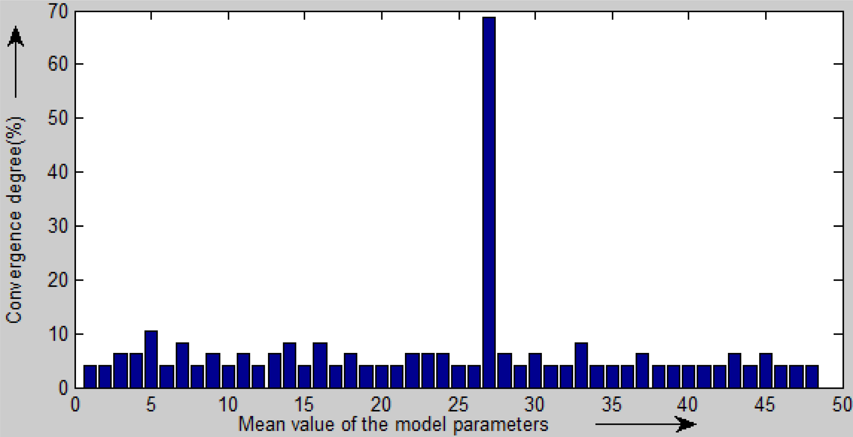
3.2.2. Fitting Process Based on the Improved BaySAC Algorithm

A well-regarded technique for robust model fitting of point clouds is the statistical framework of RANSAC (RANdom SAmple Consensus) [21], which tries many minimal random subsets and evaluates the fit of each subset's model. However, the original RANSAC algorithm assumes constant prior probabilities for the data points and randomly chooses the initial data sets, which likely leads to more iterations and expensive computational costs when the hypothesis set is contaminated by many outliers.

To improve the computational efficiency, this study employs a conditional sampling method based on BaySAC (Bayesian SAmpling Consensus) [23], which always selects the minimum number of data required with the highest inlier probabilities as a hypothesis set and thus reduces the number of iterations needed to find a good model. Instead of using specific characteristic information about a primitive, the improved BaySAC algorithm computes the prior probability of each data point using statistical testing of candidate model parameters. Moreover, the probability update is implemented using the simplified Bayes' formula. Compared with RANSAC, the key properties of the improved BaySAC algorithm are to determine and update the prior probabilities of the data points. For details of the algorithm, please refer to Kang et al. [23].

After the quadric parametric surface parameters are determined, a cross-sectional point is interpolated by computing the intersection point of the fitted surface and the radial line along the extraction direction. Figure 7a shows the cross-sectional points that are extracted to represent the cross section. Several noisy points, such as those on wires and pipelines, are included in the set and should be eliminated. Because the standard shape of the subway tunnel of interest is a circle, circle fitting is implemented using RANSAC to remove the irrelevant points and to retain the real cross-sectional points; thus, the cross section is extracted (Figure 7b) in a circular form.

4. Experimental Section

The proposed approach was tested on a real dataset (Figure 8), which was acquired using a RIEGL LMS VZ-400 laser scanner in a subway tunnel in Shanghai, China.

Table 1. Description of the point cloud dataset.

Laser Scanner	Scan Angular Resolution	n	Range Accuracy
RIEGL VZ-400	0.046°	2,686,866	±5 mm

Note: n is the total number of TLS points in the dataset.

describes the point cloud dataset.

4.1. Central Axis Fitting

4.1.1. Fitting of the Central Axis Based on the 2D Projection

As proposed in Section 2.1, the tunnel points of the VZ-400 dataset were projected onto the XOY plane as shown in Figure 9. The boundary points were extracted and are shown by the dark dots.

As presented in Section 2.1.2, the bounding lines of a tunnel may comprise segments of straight lines, curves and transition curves. The proposed statistical testing algorithm was implemented using the three models to automatically detect the corresponding initial model from the extracted boundary points. Figure 10 shows the peaks in the histograms for the straight lines, transition curves and curves of the extracted boundary points that were fit using the three models.

Based on the detected initial model (e.g., the transition curve), we fit the bounding lines using RANSAC (Figure 11a). The boundary points were evenly resampled in terms of the fitted model parameters. The method presented in Section 2.1 was implemented using these fitted parameters to extract the central-axis points (Figure 11b). Figure 11c shows a 3D view of the central axis that was generated from the central-axis points.

As shown in Figure 12, the central axis fitted from the tunnel points consists of three segments. The yellow box on the left highlights the overlap between the curve and the transition curve, while the box on the right shows the overlap between the transition curve and the straight line. To test the fitting accuracy, we set 24 Y coordinates along the central axis within the overlap zones highlighted in the two yellow boxes. Their corresponding points on the two adjacent segments were computed. The deviations between the corresponding points were then calculated and are shown in

Table 2. Comparison of the fitting accuracies.

ID	Deviations after Global Extraction (m)	Deviations before Global Extraction (m)	ID	Deviations after Global Extraction (m)	Deviations before Global Extraction (m)
1	0.005	0.035	13	0.001	0.056
2	−0.003	−0.026	14	0.004	0.039
3	0.002	0.019	15	−0.005	0.022
4	0.003	0.016	16	0.003	0.047
5	−0.005	0.002	17	0.001	−0.032
6	0.001	0.001	18	0.004	0.03
7	−0.003	−0.007	19	0.001	0.038
8	0.002	0.003	20	−0.007	−0.015
9	−0.001	0.008	21	−0.001	0.035
10	−0.003	0.004	22	0.003	0.002
11	0.0013	0.01	23	0.001	−0.025
12	−0.002	−0.035	24	0.002	0.015
RMSE				0.002	0.026

. Large deviations with an RMSE of 26 mm (the zoom-in views) are present within the overlap zones between the segments due to the noise in the tunnel point dataset.

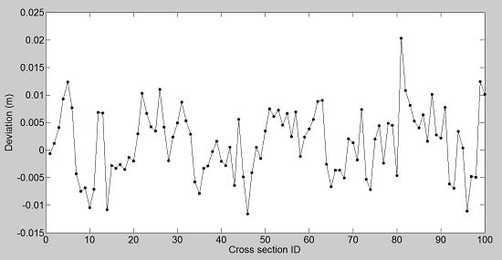
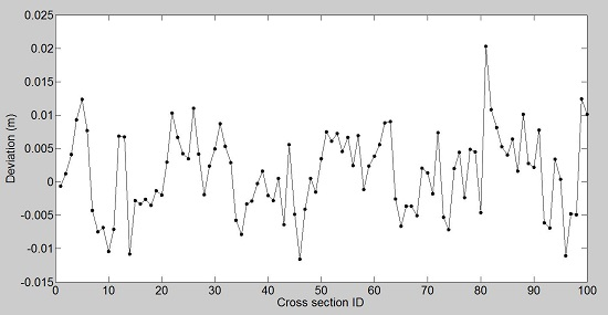
4.1.2. Global Extraction of the Central Axis Using Segment-Wise Fitting

To optimize the extraction result, the global least squares adjustment proposed in Section 2.2 was implemented to minimize the deviations in the overlap zones between the adjacent fitted models. Figure 13 shows that the differences in Figure 12 were remarkably reduced, and a globally optimized central axis was extracted.

To test the fitting accuracy, we set 24 Y coordinates along the central axis within the overlap zones highlighted in the two yellow boxes. Their corresponding points on the two adjacent segments were computed. The deviations between the corresponding points were then calculated and are shown in Table 2. The RMSE of the deviations was reduced from 26 mm to 2 mm by the global extraction process.

4.2. Cross Section Extraction Based on Quadric Parametric Surface Fitting

As presented in Section 2.2, the proposed algorithm for the continuous extraction of cross sections must interpolate a large number of cross-sectional points. The interpolation of a cross-sectional point involves the fitting of a quadric parametric surface. Therefore, we implemented the improved BaySAC algorithm described in Section 3.2.2 to improve the computational efficiency and the robustness of the quadric parametric surface fitting. In this section, the performances of the quadric parametric surface fitting using the optimized BaySAC algorithm and the RANSAC framework were compared in terms of their computational efficiencies and fitting accuracies.

4.2.1. Computational Efficiency

Because hypothesis testing is an iterative process, the computational efficiencies of the proposed strategies were evaluated in terms of the number of iterations. The iterations of RANSAC are shown as circular icons in Figure 14. The horizontal and vertical axes in Figure 14 represent the numbers of fitted laser point subsets and the number of iterations, respectively. For example, the green circle (3,020, 97) indicates that 97 iterations were required to fit a quadric parametric surface to a subset of 3,020 points using RANSAC. As described in Section 3.2.2, the iterations of BaySAC-ST (Statistical Testing) include two parts: the random part and BaySAC. These parts are depicted using square and diamond icons, respectively. The random part consists of the iterations that are required to determine the prior probability using statistical testing of the candidate model parameters sets.

As shown in Figure 14, when the number of laser points in the fitted subsets increases, the number of iterations of RANSAC also increases. When using BaySAC-ST, it generally takes fewer than 50 iterations to determine the prior probability using statistical testing of the candidate model parameters sets. As presented in Section 2, after determining the prior probability of every data point, the hypothesis testing strategy changes from RANSAC to BaySAC. Figure 14 shows a remarkable decrease in the number of iterations compared to RANSAC. For example, the fitting of a subset of 5,010 points using RANSAC requires 267 iterations, whereas the BaySAC requires only 103 iterations.

4.2.2. Fitting Accuracy

Figure 15 illustrates the fitting results of the RANSAC and the optimized BaySAC algorithms on a subset of 1,298 tunnel points that were extracted along the vertical angle (such as the 330° direction) of a cross section. To visualize the difference in the fitting accuracy, Figure 15 shows the front (left) and side (middle) views of the fitting results, where the diamond-shaped points denote the original laser points, and the grey curves represent the fitted primitives (side view). The right section of Figure 15a (a zoomed-in view of the region highlighted by a rectangle in the middle part) shows that the fitted surface acquired by RANSAC fits the lower point segment well; however, it clearly deviates from the upper segment. The right section of Figure 15b illustrates a more optimized fit; the inliers are evenly distributed around the fitted surface, which was achieved using the proposed optimized BaySAC algorithm.

To further test the fitting accuracy, we selected ten inliers as check points. The point-to-surface distances were then calculated and are shown in

Table 3. Accuracies of quadric parametric surface fitting.

Point	Point-to-Surface Distance (m)
	RANSAC	Optimized BaySAC
1	0.0021	0.0009
2	0.0020	0.0009
3	0.0008	0.0002
4	0.0012	0.0005
5	0.0016	0.0007
6	0.0025	0.0015
7	0.0019	0.0010
8	0.0010	0.0007
9	0.0020	0.0015
10	0.0014	0.0009

. The maximum, minimum and average point-to-surface distances from RANSAC are 2.5 mm, 0.8 mm and 1.6 mm, respectively, whereas those from BaySAC are 1.5 mm, 0.2 mm and 0.9 mm. The results indicate that the optimized BaySAC algorithm achieved a higher overall fitting accuracy.

As described in Section 3.2, we proposed an algorithm to interpolate cross-sectional points using quadric parametric surface fitting when no cross-sectional point can be directly acquired from the laser points. To evaluate the accuracy of the interpolation, five laser points were chosen, and their interpolated coordinates were computed, as shown in

Table 4. Accuracy of the cross-sectional point interpolation.

ID	Measured Coordinates (m)			Interpolated Coordinates (m)			Deviation (m)
	X	Y	Z	X	Y	Z
1	−3.171	15.578	0.051	−3.1705	15.578	0.0510	0.0005
2	−3.182	15.544	0.013	−3.1821	15.544	0.1330	0.0001
3	−2.842	15.680	1.918	−2.8409	15.680	1.9173	0.0013
4	−2.864	15.759	1.875	−2.8646	15.759	1.8754	0.0007
5	−0.596	15.576	−1.573	0.5965	15.576	−1.5744	0.0015
Mean deviation (m)							0.0008

. The mean deviation of the interpolated coordinates from the measured points is only 0.8 mm.

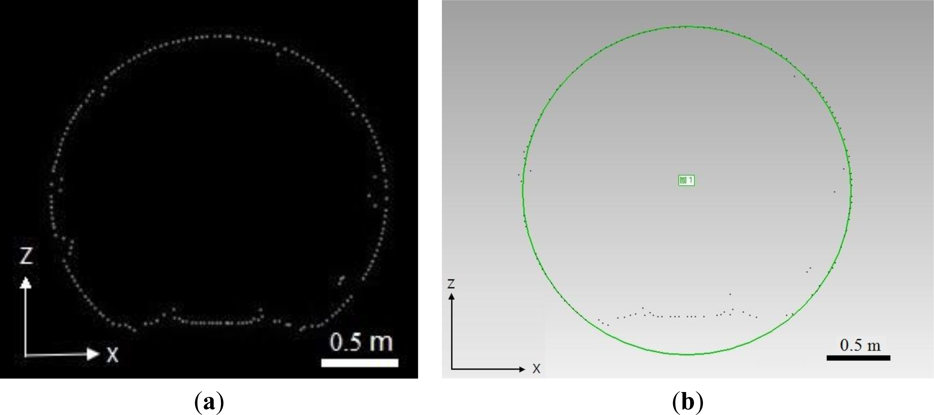
4.2.3. Continuous Extraction of the Cross Sections

As mentioned in Section 3, our proposed algorithm can theoretically extract cross sections at any interval from the terrestrial point clouds. We implemented the cross section extraction experiments at a one-meter interval. The average computational cost of the cross section extraction was less than 3 s/section. The candidate cross-sectional points were extracted using the straight line that was orthogonal to the central axis of the tunnel within a vertical plane at a one-degree interval (Figure 16a). Noise points from wires and pipelines are clearly present in the data. As proposed in Section 3, circle fitting was implemented using RANSAC to remove the irrelevant points (Figure 16b). An overview of all extracted cross sections is shown in Figure 16c.

To evaluate the accuracy of the cross section fitting, 100 cross sections were fitted from the VZ-400 data. Because the standard shape of the tunnel cross section of interest is a circle, the radii of the fitted circular cross sections were compared with the design radius of 2.75 m. Figure 17 illustrates the differences between the cross sections and the design, which have a standard deviation of 6 mm.

Moreover, the chord length between every two cross-sectional points was calculated (e.g., Figure 18). We regarded the chord lengths of two different cross sections as corresponding chord lengths if the chord lengths were computed using the cross-sectional points selected in different cross sections with the same vertical angles. The corresponding chord lengths were then compared. Figure 19 shows the deviations between the corresponding chord lengths. The average lengths of chord I and II are 3.6487 m and 5.0951 m, respectively, and the standard deviations are 1.4 mm and 1 mm.

5. Conclusions

In this paper, we proposed an efficient algorithm to continuously extract tunnel cross sections. First, the central axis of a subway tunnel was extracted using multiple model fitting based on 2D projections of a tunnel point cloud. This axis was optimized using a global extraction strategy based on segment-wise fitting. After the central axis was determined, the cross section was extracted by intersecting a radial line that orthogonally rotates about the central axis of the tunnel point cloud. An interpolation algorithm based on quadric parametric surface fitting using an improved BaySAC (Bayesian SAmpling Consensus) algorithm was proposed to compute a cross-sectional point when no cross-sectional point could be directly acquired from the tunnel points along the direction of interest. Because the standard shape of the tunnel cross section of interest is a circle, circle fitting was implemented using RANSAC (RANdom SAmple Consensus) to filter the noise.

The proposed algorithm was implemented using a terrestrial laser scanning dataset that was acquired in a subway tunnel. The results of the central-axis extraction show that the proposed algorithm of global extraction based on segment-wise fitting achieved an accuracy of 2 mm, while the accuracy acquired by the fitting based on a single model is 26 mm. The results of the cross section extraction process show that the interpolation of the cross-axial points based on the improved BaySAC algorithm produces a mean deviation of 0.9 mm from the measured points. The millimeter-level accuracies (6 mm, 1.4 mm and 1 mm) of the cross section extraction were demonstrated respectively by comparing the fitted radii with the designed radius of the cross section in the subway and comparing corresponding chord lengths in different cross sections. Moreover, the average computational cost of the cross section extraction method was less than 3 s/section, which demonstrates its high efficiency.

Because variations in the scanning parameters, such as point density, range to the scanner and incidence angle, and can affect the quality of the results, their effects and the optimization of the scanning parameters will be investigated in subsequent studies. Moreover, the deformation tendency of a tunnel can be reflected by the variance of its radius among the fitted circular cross sections and the variance between corresponding chord lengths in different cross sections. Future work will also focus on optimizing the proposed algorithm to detect possible deformation based on so-called continuously extracted cross sections.

References

1. Wang, T.-T.; Jaw, J.-J.; Chang, Y.-H.; Jeng, F.-S. Application and validation of profile-image method for measuring deformation of tunnel wall. Tunn. Undergr. Space Technol. 2009, 24, 136–147. [Google Scholar]
2. Paar, G.; Kontrus, H. Three-Dimensional Tunnel Reconstruction Using Photogrammetry and Lasers Scanning. Proceedings of the 3rd Nordost, 9. Anwendungsbezogener Workshop zur Erfassung, Modellierung, Verarbeitung und Auswertung von 3D-Daten, Berlin, Germany, 1 December 2006.
3. Tsakiri, M.; Lichti, D.; Pfeifer, N. Terrestrial Laser Scanning for Deformation Monitoring. Proceedings of the 3rd IAG/12th FIG Symposium, Baden, Austria, 22–24 May 2006.
4. Gordon, S.J.; Lichti, D.D. Modeling terrestrial laser scanner data for precise structural deformation measurement. ASCE J. Surv. Eng 2007, 133, 72–80. [Google Scholar]
5. Van Gosliga, R.; Lindenbergh, R.; Pfeifer, N. Deformation analysis of a bored tunnel by means of terrestrial laser scanning, international archives of photogrammetry. Remote Sens. Spat. Inf. Sci 2006, 36, 167–172. [Google Scholar]
6. Lindenbergh, R.; Uchanski, L.; Bucksch, A.; Gosliga, R. Structural monitoring of tunnels using terrestrial laser scanning. Rep. Geod 2009, 87, 231–239. [Google Scholar]
7. Schneider, D. Terrestrial Laser Scanner for Area Based Deformation Analysis of Towers and Water Damns. Proceedings of the 3rd IAG Symposium of Geodesy for Geotechnical and Structural Engineering and 12th FIG Symposium on Deformation Measurements, Baden, Austria, 22–24 May 2006; p. 6.
8. Monserrat, O.; Crosetto, M. Deformation measurement using terrestrial laser scanning data and least squares 3D surface matching. ISPRS J. Photogramm. Remote Sens 2008, 63, 142–154. [Google Scholar]
9. Gruen, A.; Akca, D. Least squares 3D surface and curve matching. ISPRS J. Photogramm. Remote Sens 2005, 59, 151–174. [Google Scholar]
10. Pejic', M. Design and optimisation of laser scanning for tunnels geometry inspection. Tunn. Undergr. Space Technol 2013, 37, 199–206. [Google Scholar]
11. Yoon, J.; Sagong, M.; Lee, J.S.; Lee, K. Feature extraction of a concrete tunnel liner from 3D laser scanning data. NDT E Int 2009, 42, 97–105. [Google Scholar]
12. Gikas, V. Three-dimensional laser scanning for geometry documentation and construction management of highway tunnels during excavation. Sensors 2012, 12, 11249–11270. [Google Scholar]
13. Seo, D.-J.; Lee, J.C.; Lee, Y.-D.; Lee, Y.-H.; Mun, D.-Y. Development of cross section management system in tunnel using terrestrial laser scanning technique. Int. Arch. Photogramm. Remote Sens. Spat. Inf. Sci 2008, 37, 573–581. [Google Scholar]
14. Slob, S.; Hack, H.R.G.K. 3D Terrestrial Laser Scanning as a New Field Measurement and Monitoring Technique. In Engineering Geology for Infrastructure Planning in Europe: A European Perspective; Robert, H., Rafig, A., Robert, C., Eds.; Springer Verlag: Berlin, Germany, 2004; pp. 179–190. [Google Scholar]
15. Han, S.; Cho, H.; Kim, S.; Jung, J.; Heo, J. Automated and efficient method for extraction of tunnel cross sections using terrestrial laser scanned data. J. Comput. Civ. Eng 2013, 27, 274–281. [Google Scholar]
16. Kang, Z.; Tuo, L.; Zlatanova, S. Continuously deformation monitoring of subway tunnel based on terrestrial point clouds. Int. Arch. Photogramm. Remote Sens. Spat. Inf. Sci 2012, XXXIX-B5, 199–203. [Google Scholar]
17. Oude Elberink, S.; Khoshelham, K.; Arastounia, M.; Díaz Benito, D. Rail track detection and modelling in mobile laser scanner data. ISPRS Ann. Photogramm. Remote Sens. Spat. Inf. Sci 2013, II-5/W2, 223–228. [Google Scholar]
18. Telea, A.; van Wijk, J. An Augmented Fast Marching Method for Computing Skeletons and Centrelines. Proceedings of the Symposium on Data Visualisation, Barcelona, Spain, 27–29 May 2002; pp. 251–259.
19. Pock, T.; Beichel, R.; Bischof, H. A novel robust tube detection filter for 3D centerline extraction. Lect. Notes Comput. Sci 2005, 3540, 55–94. [Google Scholar]
20. Hassouna, M.S. Robust Centerline Extraction Framework Using Level Sets. Proceedings of the IEEE Computer Society Conference on Computer Vision and Pattern Recognition (CVPR 2005), New York, NY, USA, 20–25 June 2005; pp. 458–465.
21. Fischler, M.A.; Bolles, R.C. Random sample consensus: A paradigm for model fitting with applications to image analysis and automated cartography. ACM Commun 1981, 24, 381–395. [Google Scholar]
22. Yang, M.; Lee, E. Segmentation of measured data using a parametric quadric surface approximation. Comput. Aided Des 1999, 31, 449–457. [Google Scholar]
23. Kang, Z.; Zhang, L.; Wang, B.; Li, Z.; Jia, F. An optimized BaySAC algorithm for efficient fitting of primitives in point clouds. IEEE. Geosci. Remote Sens. Lett. 2013. [Google Scholar] [CrossRef]
Figure 1. Extraction of boundary points using a moving window.
Remotesensing 06 00857f1
Figure 2. Histogram of hypothesis model parameters.
Remotesensing 06 00857f2
Figure 3. Determination of the central-axis point.
Remotesensing 06 00857f3
Figure 4. Segment-wise fitting.
Remotesensing 06 00857f4
Figure 5. Adjustment of the pseudo cross-sectional plane [15]. (a) Plan view; (b) Perspective view.
Remotesensing 06 00857f5
Figure 6. Cross-sectional point estimation.
Remotesensing 06 00857f6
Figure 7. Extraction of the cross section. (a) Extracted cross-sectional points; (b) The real cross-sectional points.
Remotesensing 06 00857f7
Figure 8. The experimental dataset.
Remotesensing 06 00857f8
Figure 9. 2D projection of the tunnel points onto the XOY plane.
Remotesensing 06 00857f9
Figure 10. Statistical test results of the optimized BaySAC algorithm. (a) Straight line; (b) Transition curve; (c) Curve.
Remotesensing 06 00857f10
Figure 11. Fitting of the tunnel axis (the transition curve). (a) Fitted bounding lines; (b) Central-axis extraction; (c) Extracted 3D central axis.
Remotesensing 06 00857f11
Figure 12. Extracted central axis.
Remotesensing 06 00857f12
Figure 13. Central-axis fitting with global least squares adjustment.
Remotesensing 06 00857f13
Figure 14. Computational efficiency.
Remotesensing 06 00857f14
Figure 15. Fitting results of the laser point subset of a tunnel. (a) RANSAC; (b) Optimized BaySAC.
Remotesensing 06 00857f15
Figure 16. Cross section extraction. (a) Interpolated candidate cross-sectional points; (b) Real cross-sectional points extracted by RANSAC; (c) Overview of all extracted cross sections.
Remotesensing 06 00857f16
Figure 17. Deviations between the fitted radii and the designed radius.
Remotesensing 06 00857f17
Figure 18. Chords used for comparison. (a) Chord I; (b) Chord II.
Remotesensing 06 00857f18
Figure 19. Comparison of corresponding chord lengths. (a) Chord I; (b) Chord II.
Remotesensing 06 00857f19