Article

Validation and Application of the Modified Satellite-Based Priestley-Taylor Algorithm for Mapping Terrestrial Evapotranspiration

1
State Key Laboratory of Remote Sensing Science, College of Global Change and Earth System Science, Beijing Normal University, No.19 Xinjiekou Street, Beijing 100875, China
2
Department of Geographical Sciences, University of Maryland, College Park, MD 20742, USA
3
Ministry of Environmental Protection, Environmental Satellite Center, East Road of Yongfeng Base, Beijing 100094, China
4
College of Resource Environment and Tourism, Capital Normal University, No.105 North Road, Beijing 100048, China
5
Institute of Remote Sensing and GIS, Peking University, No.5 Yiheyuan Road, Beijing 100871, China
6
School of Earth Sciences and Engineering, Hohai University, No.1 Xikang Road, Nanjing, 210098, China
7
College of Earth Sciences, Chengdu University of Technology, No.1 Erxian Bridge Road, Chengdu 610059, China
*
Author to whom correspondence should be addressed.
Remote Sens. 2014, 6(1), 880-904; https://doi.org/10.3390/rs6010880
Submission received: 24 November 2013 / Revised: 2 January 2014 / Accepted: 3 January 2014 / Published: 17 January 2014

Abstract

:
Satellite-based vegetation indices (VIs) and Apparent Thermal Inertia (ATI) derived from temperature change provide valuable information for estimating evapotranspiration (LE) and detecting the onset and severity of drought. The modified satellite-based Priestley-Taylor (MS-PT) algorithm that we developed earlier, coupling both VI and ATI, is validated based on observed data from 40 flux towers distributed across the world on all continents. The validation results illustrate that the daily LE can be estimated with the Root Mean Square Error (RMSE) varying from 10.7 W/m2 to 87.6 W/m2, and with the square of correlation coefficient (R2) from 0.41 to 0.89 (p < 0.01). Compared with the Priestley-Taylor-based LE (PT-JPL) algorithm, the MS-PT algorithm improves the LE estimates at most flux tower sites. Importantly, the MS-PT algorithm is also satisfactory in reproducing the inter-annual variability at flux tower sites with at least five years of data. The R2 between measured and predicted annual LE anomalies is 0.42 (p = 0.02). The MS-PT algorithm is then applied to detect the variations of long-term terrestrial LE over Three-North Shelter Forest Region of China and to monitor global land surface drought. The MS-PT algorithm described here demonstrates the ability to map regional terrestrial LE and identify global soil moisture stress, without requiring precipitation information.

1. Introduction

Evapotranspiration (LE) is a major component of the earth’s climate system and global water cycle, and it represents a crucial link between global water, energy and carbon exchanges [14]. Although the current Eddy Covariance (ECOR) or Bowen Ratio (BR) systems at flux towers have provided point measurements of terrestrial LE, LE is inherently difficult to measure and predict especially at large spatial scales because sufficient ground observations will never be available [35]. In contrast, remotely sensed data can be used as proxies for retrieving important controlling variables. Therefore, satellite-based estimate of temporal and spatial variations of LE is crucial for improving hydrological and agricultural management [610].
Advances in satellite-based LE algorithms and remote sensing technology enable estimating terrestrial LE at regional or global scales [721]. Comprehensive reviews of the historical development and accuracies of in situ and satellite-based LE estimation methods are provided elsewhere [3,5,22]. These LE methods mainly include the simplified empirical (SE) method [2,23,24], surface energy balance (SEB) based single-and dual-source models [11,25,26], Penman-Monteith (PM) equation [8,1416,27], and data assimilation (DA) techniques [2830]. Although great progress has been made on remotely sensed estimation of LE at a regional scale with these models, there are still challenges and limitations that have not yet been solved properly. For example, the aerodynamic resistances of PM equation require knowledge about atmospheric stability, and several vegetation and soil parameters, as well as meteorological data [15,16,31,32]. However, such surface meteorological observations are not readily available over large areas. Similarly, many empirical LE methods are usually calibrated for specific regions and their robustness across multiple regions has not been systematically evaluated.
An alternative approach, the Priestley-Taylor (PT) algorithm, can be accurate where aerodynamic and surface resistance is not available and a coefficient multiplier, alpha, sets the equation equal to potential LE (PE) [17,21,3336]. The general form of the Priestley-Taylor algorithm is:
LE = α Δ Δ + γ ( R n G )
where LE is evapotranspiration in W/m2, Δ is the slope of the saturated vapor pressure curve (kPa/°C), and γ is the psychrometric constant (kPa/°C). Rn and G represent the surface net radiation and the soil heat flux in Wm−2. a is the PT coefficient. LE cannot exceed RnG without significant advection and convection. a has a limited range between 0 and (Δ + γ)/Δ and in the standard application of the Priestley-Taylor method, a equals to 1.26 over water or wet surfaces. a affects the partition of the sensible and latent heat flux because the variation of air temperature can lead to the changes of both (Δ + γ)/Δ and sensible heat flux. Generally, (Δ + γ)/Δ can vary from −2.6% to −0.7% when air temperature increases from 10 °C to 40 °C [10,37].
Based on the Priestley-Taylor algorithm, a large number of revised approaches to estimate terrestrial LE have been built. Three types of schemes have been developed to parameterize Priestley-Taylor coefficient (a) from remotely sensed data: (1) two-step interpolation scheme from the dry and wet edges in the Land Surface Temperature (LST)-Normalized Difference Vegetation Index (NDVI) triangular space [10,3743]; (2) eco-physiological constraints derived from vegetation indices (VIs) or vegetation fraction cover (fc) [2,1113,17,21,34,4446]; and (3) the parameterization of key variables characterizing soil moisture using meteorological or remotely sensed data [17,18,21,35]. However, deriving surface parameters from the vertex of LST-NDVI scatter-plots requires a continuum of soil moisture and vegetation status to provide a range of surface conditions and this method can not be applied under bare soil or full vegetation cover conditions. In addition, many parameterization schemes still need many variables, such as relative humidity (RH) or precipitation, to improve the complexity of the Priestley-Taylor algorithms, and errors derived from many input variables introduce the uncertainty of LE estimations.
To overcome the difficulty of the satellite-based estimation of relative humidity (RH) and vapor pressure deficit (VPD) for traditional Priestley-Taylor algorithm, Yao et al. [21] developed a modified satellite-based Priestley-Taylor (MS-PT) algorithm using the Apparent Thermal Inertia (ATI) derived from the temperature change and NDVI derived from remote sensing products. This model was validated over 16 eddy covariance flux towers in China with an average R2 of 0.86 and 9% bias, and applied to analyze the variations of terrestrial LE in China [21]. However, this algorithm has not been analyzed and validated its efficacy in LE estimation at other regions. Moreover, this algorithm has only used to detect the variations of LE in China, between 2001 and 2010, due to the short-term sparse regional measurement datasets.
In this study, we present an overview and validation of the modeling algorithm, and describe two current international projects involving hydrological impacts of Three-North Shelter Forest region of China and global surface drought monitoring. It has three major objectives. First, we validate the modified satellite-based Priestley-Taylor algorithm (MS-PT), based on ground-observed data from 40 flux towers distributed across the world on all continents. Second, we evaluate both MS-PT algorithm and PT-JPL algorithm based on flux towers data. Finally, we calculate decadal variation in LE of the Three-North Shelter Forest region of China during 1984–2010 and detect the trends of global land surface drought from 1984–2007.

2. Methods and Data Sources

2.1. Methods

2.1.1. MS-PT Algorithm

The modified satellite-based Priestley-Taylor algorithm (MS-PT) [21] was specifically designed to minimize the need for ancillary meteorological data while maintaining a physically realistic representation of evapotranspiration process. It only needs four variables, as follows: surface net radiation (Rn), air temperature (Ta), diurnal air temperature range (DT), and NDVI.
MS-PT algorithm estimate LE by calculating the sum of the unsaturated soil evaporation (LEs), the canopy transpiration (LEc), the saturated wet soil surface evaporation (LEws), and the canopy interception evaporation (LEic) (Figure 1). The total LE can be expressed as:
LE = LE s + LE c + LE ws + LE ic
Unsaturated soil evaporation can be calculated using an index of soil water deficit (fsm) and fsm can be acquired from an exponential algorithm of the Apparent Thermal Inertia (ATI), namely,
LE s = α ( 1 f wet ) f sm Δ Δ + γ ( R ns G )
f sm = ( 1 DT ) DT / DT max
f wet = f sm 4
where fwet is the wet surface fraction and can be derived from fsm, DTmax is the maximum diurnal air temperature range (DTmax = 40 °C), Rns is the surface net radiation to the soil and can be calculated using both Rn and vegetation cover fraction (fc) (Rns = Rn (1 − fc)). G is also derived from Rn and fc (ag(1 − fc)Rn, ag = 0.18). In MS-PT algorithm, we calculated fc using NDVI:
f c = NDVI NDVI min NDVI max NDVI min
where NDVImin and NDVImax were the minimum and maximum NDVI during the study period, set as constants of 0.05 and 0.95 [7,21], respectively.
Canopy transpiration can be estimated using the modified Linear Two-Source Model (N95) and can be described as:
LE c = α ( 1 f wet ) f T f c Δ Δ + γ R nv
f T = exp [ ( T a T opt T opt ) 2 ]
where fT is the plant temperature constraint and can be calculated using Ta and an optimum Topt set as 25 °C. Rnv is the surface net radiation to the vegetation and can be calculated using both Rn and fc (Rnv = Rnfc).
Both saturated wet soil surface evaporation and vegetation interception evaporation can be calculated from the following two equations, respectively.
LE ws = α f wet Δ Δ + γ ( R ns G )
LE ic = α f wet Δ Δ + γ R nv

2.1.2. PT-JPL Algorithm

Based on the Priestley-Taylor algorithm, Fisher et al. [17] put forward PT-JPL algorithm by downscaling potential LE from Priestley-Taylor to actual LE. PT-JPL algorithm includes many eco-physiological constraint functions by introducing atmospheric moisture (VPD and RH) and vegetation indices. The PT-JPL algorithm can be expressed as:
LE = LE i + LE c + LE s
LE i = f wet α Δ Δ + γ R nc
LE c = ( 1 f wet ) f c f T f M α Δ Δ + γ R nc
LE s = ( f wet + ( 1 f wet ) f sm ) α Δ Δ + γ ( R ns G )
where fc is the green canopy fraction (fAPAR/fIPAR), fM is a plant moisture constraint (fAPAR/fAPARmax), fsm is a soil moisture constraint (RHVPD) and fwet is the relative surface wetness (RH4), fAPAR is the absorbed photosynthetically active radiation (FPAR), fIPAR is the intercepted PAR.

2.1.3. Drought Index and Potential LE Calculations

To apply the MS-PT algorithm for global surface drought monitoring, we select the Evaporative Drought Index (EDI), incorporating actual LE and potential LE (PE), to characterize the results of soil moisture response to surface dryness [47]. The EDI can be described as:
EDI = 1 LE PE
Yao et al. [47] described the physical implications of EDI and monitored surface drought over the conterminous United States using Moderate-Resolution Imaging Spectroradiometer (MODIS) and National Centers for Environmental Prediction (NCEP) Reanalysis-2 Data. Additionally, we also adopt the Hargreaves method to estimate PE. Although the Hargreaves method mainly performs effectively for well-cropped grass, the results of EDI calculation from this method can be accepted on a global scale in this study [48]. Based on the Hargreaves model, the PE can be easily estimated from NCEP-2 data. The Hargreaves model is expressed as follows:
PE = 0.0023 R a ( T a + 17.8 ) T max T min
Here, PE is the potential evapotranspiration (mm/day) and Ra is the extraterrestrial solar incident radiation (MJ/m2 per day). Tmax is monthly maximum air temperature (°C), and Tmin is monthly minimum air temperature (°C).

2.1.4. Trend Analysis

Linear trend analysis is used to analyze the regional long-term LE trend of Three-North Shelter Forest Region of China and to explore the variation of global land surface EDI, respectively. A simple linear regression equation is used to calculate the annual values and to obtain the long-term LE and EDI trends.
y t = y 0 + bt
Here, yt represents the annual value of LE or EDI, t is the year and coefficient b represents the trend of long-term annual LE or EDI. Moreover, the Student’s t-test distribution with n − 2 degrees of freedom is adopted to calculate the confidence levels of the derived tendencies [49]. We also apply the linear trend analysis pixel-wise to calculate the trend for each pixel and calculate regional average time series, and, then, apply the linear trend analysis to quantify the regional trends.

2.2. Data

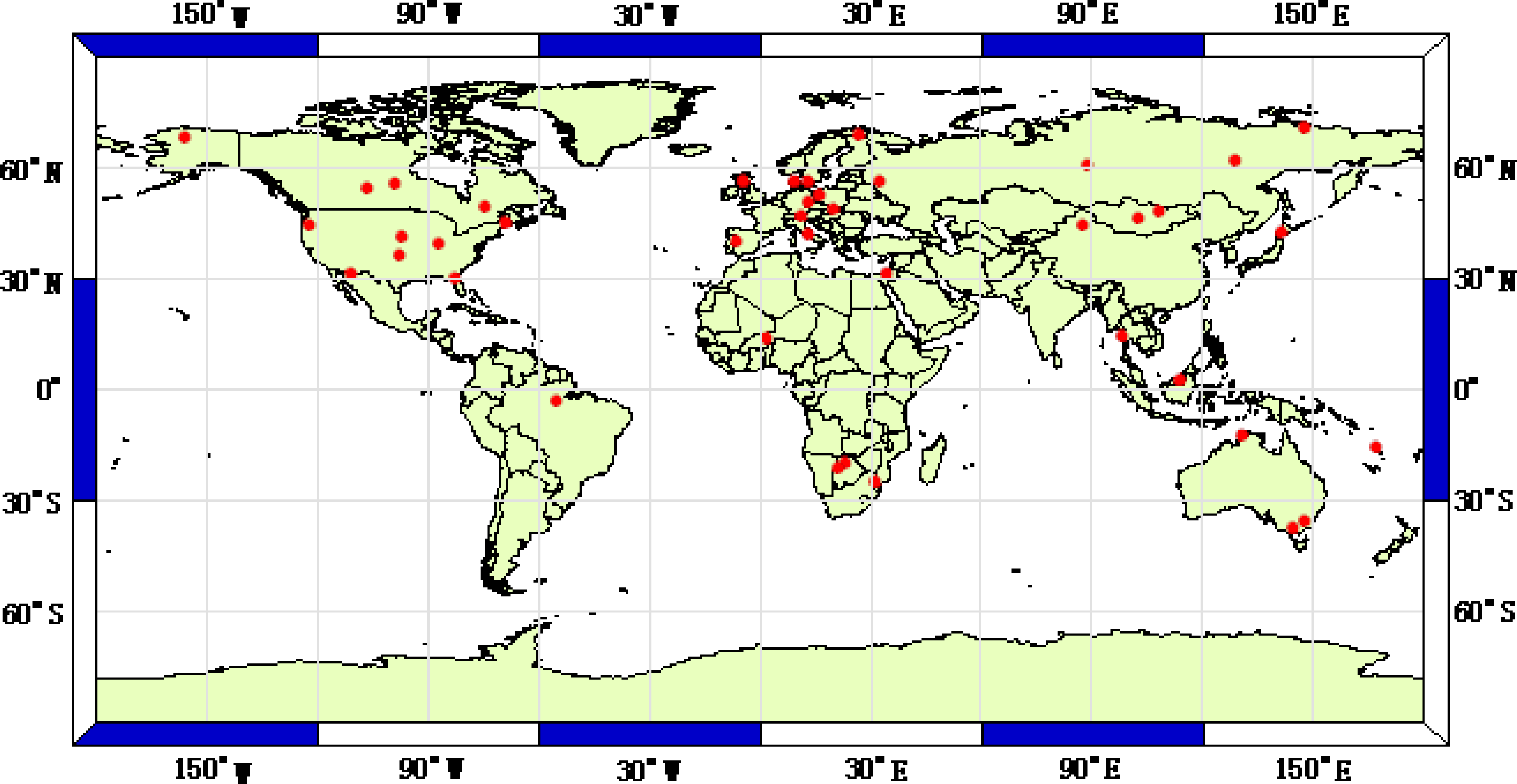
2.2.1. Eddy Covariance Flux Towers

To evaluate the performance of both MS-PT algorithm and PT-JPL algorithm, we use the ground-observed data from 40 flux towers distributed the world: ten AmeriFlux sites, five AsiaFlux sites, one Atmospheric Radiation Measurement (ARM) site, one Chinese Ecosystem Research Network (CERN) site, one Asian Automatic Weather Station Network Project (ANN) site supported by the GEWEX (Global Energy and Water cycle EXperiment) Asian Monsoon Experiment (GAME AAN) and twenty-three other flux towers sites (Table 1 and Figure 2). These data sets include the longest continuous worldwide multi-site measurements of LE, Rn, and corresponding meteorological observations, and each tower provides at least one year of reliable data. The land cover types of the flux towers sites include grasslands, crop, shrub, savanna, wetlands, evergreen forest, deciduous forest, and mixed forests (Table 1). LE collected from all flux towers is measured by the Eddy Covariance (ECOR) method. Although the ECOR method has been widely used in global measurement experiment, this method does not conserve energy [19,20]. In this study, we have selected the method developed by Twine et al. [50] to correct the LE from all flux towers.

2.2.2. Meteorological and Satellite Inputs

To validate the MS-PT algorithm, MODIS NDVI and FPAR composite products with a 1-km spatial resolution and eight-day temporal resolution are used. The daily NDVI and FPAR values are temporally interpolated from the eight-day averages using linear interpolation. To investigate long-term variability of LE over the Three-North Shelter Forest region of China during 1982–2009, we use monthly air temperature, maximum air temperature, minimum air temperature, and surface net radiation products with 0.5 × 0.67 degree spatial resolution derived from reanalysis meteorology of the Modern Era Retrospective-analysis for Research and Applications (MERRA) from NASA’s Global Modeling and Assimilation Office (GMAO). All coarse resolution GMAO-MERRA products are spatially interpolated into 0.1 degree. In addition, we use the monthly NDVI at an 8-km spatial resolution derived from the Global Inventory Modeling and Mapping Studies (GIMMS) group at the National Aeronautics and Space Administration (NASA) Goddard Space Flight Center [51], and we also interpolated NDVI into 0.1 degree.
For global land surface drought monitoring, we use global monthly surface downward and upward shortwave and long-wave radiation products at a spatial resolution of 1° × 1° from 1984 through 2007 that are derived from GEWEX Surface Radiation Budget (SRB) products. The monthly air mean temperature, and the maximum and minimum air temperature data are extracted from NCEP-2 data, which are acquired from the NCEP/NCAR Reanalysis Project (CDAS). These datasets have a spatial resolution of 1.875° longitude by approximately 1.9° latitude, and are interpolated into 1° × 1° using bilinear interpolation. The monthly GIMMIS NDVI products at a spatial resolution of 8 km are also interpolated into 1 degree. We also use the monthly Palmer Drought Severity Index (PDSI) products derived from the NCAR CGD’s Climate Analysis Section dataset with a 2.5-degree spatial resolution, for the period from 1984 through 2007. To highlight the obvious features of both PDSI and EDI, we have interpolated the PDSI products into 1 degree from a 2.5-degree spatial resolution.

3. Results and Discussion

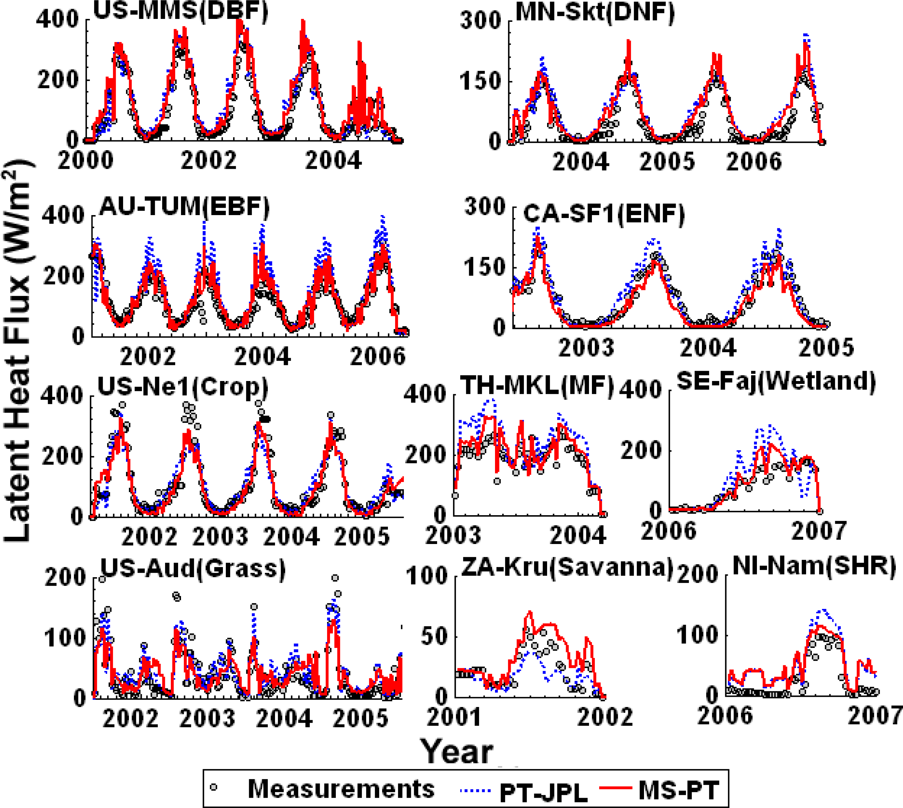
3.1. Validation and Comparison

To evaluate the ability of the MS-PT method to predict the spatial variation in LE, we have validated both MS-PT algorithm and PT-JPL algorithm based on the collected ground-measured data from all flux towers sites. Table 2 shows the Root Mean Square Error (RMSE), the bias, and the square of correlation coefficients (R2) of the comparison between the ground-measured and estimated daily LE from 40 flux towers. One can observe that the RMSE of the estimated daily LE using MS-PT algorithm varies from 10.7 W/m2 to 87.6 W/m2, the bias varies from −23.7 W/m2 to 48.6 W/m2, and R2 varies from 0.41 to 0.89 (p < 0.01). Similarly, the RMSE of the estimated daily LE using PT-JPL algorithm varies from 11.3 W/m2 to 89.1 W/m2, the bias varies from −21.3 W/m2 to 56.2 W/m2, and R2 varies from 0.40 to 0.88 (p < 0.01). Overall, as compared with PT-JPL algorithm, MS-PT algorithm improves the LE estimates at most flux towers sites.
Figure 3 shows an example of the eight-day time series of modeled LE, using both MS-PT algorithm and PT-JPL algorithm driven by tower daily meteorological measurements versus the corresponding tower LE measurements. The results illustrate MS-PT algorithm performs better than PT-JPL algorithm. The MS-PT algorithm provides the favorable agreement with the tower observations and captures observed LE seasonality and associated differences among the major land cover types. Figure 4 illustrates scatter plots of a comparison between annual estimated and ground-measured LE using MS-PT algorithm driven by the ground observations. We notice that the bias of the estimated LE at all 40 flux towers sites is 2.5 W/m2. The RMSE is 28.4 W/m2 and the R2 is 0.68 (p < 0.01). The accuracy of the LE simulation can be used for estimating the regional or global land surface LE. As the flux towers sites have different land cover types and different climate regimes, the comparison of the site-averaged LE demonstrates the ability of this method to predict the spatial variation in LE.
To fairly assess how well the model predicts long-term variations in LE, we have validated the estimated annual LE anomalies with the observed annual LE anomalies. We only use flux towers sites where five years of data are available. As shown in Figure 5, the bias of estimated annual LE anomalies deviating from ground-based observations is −2.3 W/m2, the RMSE is 11.2 W/m2 and R2 is 0.42 (p = 0.02). This illustrates that the annual variation of LE is slightly smaller than that expected and perhaps the missing NDVI caused by bad weather can explain this small bias [19,20]. In general, MS-PT algorithm works well, indicating that this method may be a good tool for detecting the long-term variation of LE.
Rigorous validation of the surface latent heat flux derived from remote sensing data is a challenging scientific problem as soil surface evaporation and plant transpiration involve complicated physical processes The differences in the performance of our MS-PT algorithm among different land cover types or locations are partly caused by errors of ground-observations over flux towers, landscape heterogeneity over flux sites, and the limitations of the MS-PT algorithm. One source that may influence the performance of LE modeling is the flux measurement itself. These flux measurements use the ECOR method to obtain surface radiation fluxes and ECOR suffers energy imbalance. Although we have selected the method proposed by Twine et al. [50] to correct LE, the uncertainty of observed LE still exists. In addition, the quality of MODIS NDVI products also affects the biases of validations. Heterogeneity within the subset around flux towers may influence the correlation between field measurements and remote sensing simulation due to mismatch in spatial representative areas [52,53]. MODIS NDVI products are still average values in a given pixel (large area) and often mix with signals of lower vegetation, which will lead to errors in LE modeling among different ecological categories. Another source that can account for the differences between the observed LE from flux towers and the modeled LE is the limitations of the MS-PT algorithm, which neglects the differences of parameters in different biome types. Thus, there may be small biases between the observed and the modeled LE.
Accurate validations of soil evaporation and vegetation transpiration are difficult because of the deficiency of bare soil flux towers sites. In this study, we only use a simple NDVI-based equation to calculate vegetation cover. In fact, for different land cover types, vegetation cover calculation is difficult because for most land cover types, smaller NDVI values correspond to winter values and thus have larger uncertainties due to cloud contamination and atmospheric effects than in the summer [54,55]. Therefore, if the fraction of bare soil is miscalculated, the evaporation from the soil fraction based on thermal inertial will be off, as will transpiration from the canopy fraction. It is possible these are compensating errors that reduce overall error. Similarly, for the canopy, it is assumed that the vegetated fraction will transpire at a rate determined by Rn with a fixed alpha value, moderated by the vegetation cover and optimal temperature. In fact, stomatal conductance is sensitive to a number of environmental factors and many variables can not be acquired only using remotely sensed data. In this study, we use vegetation cover derived from NDVI to represent the variations in vegetation state and canopy response to changes in environmental conditions such as water availability in the vegetation root zone, the plant water potential, FPAR and CO2 concentration [56,57]. Large error and uncertainty may be introduced by these approximations and assumptions.

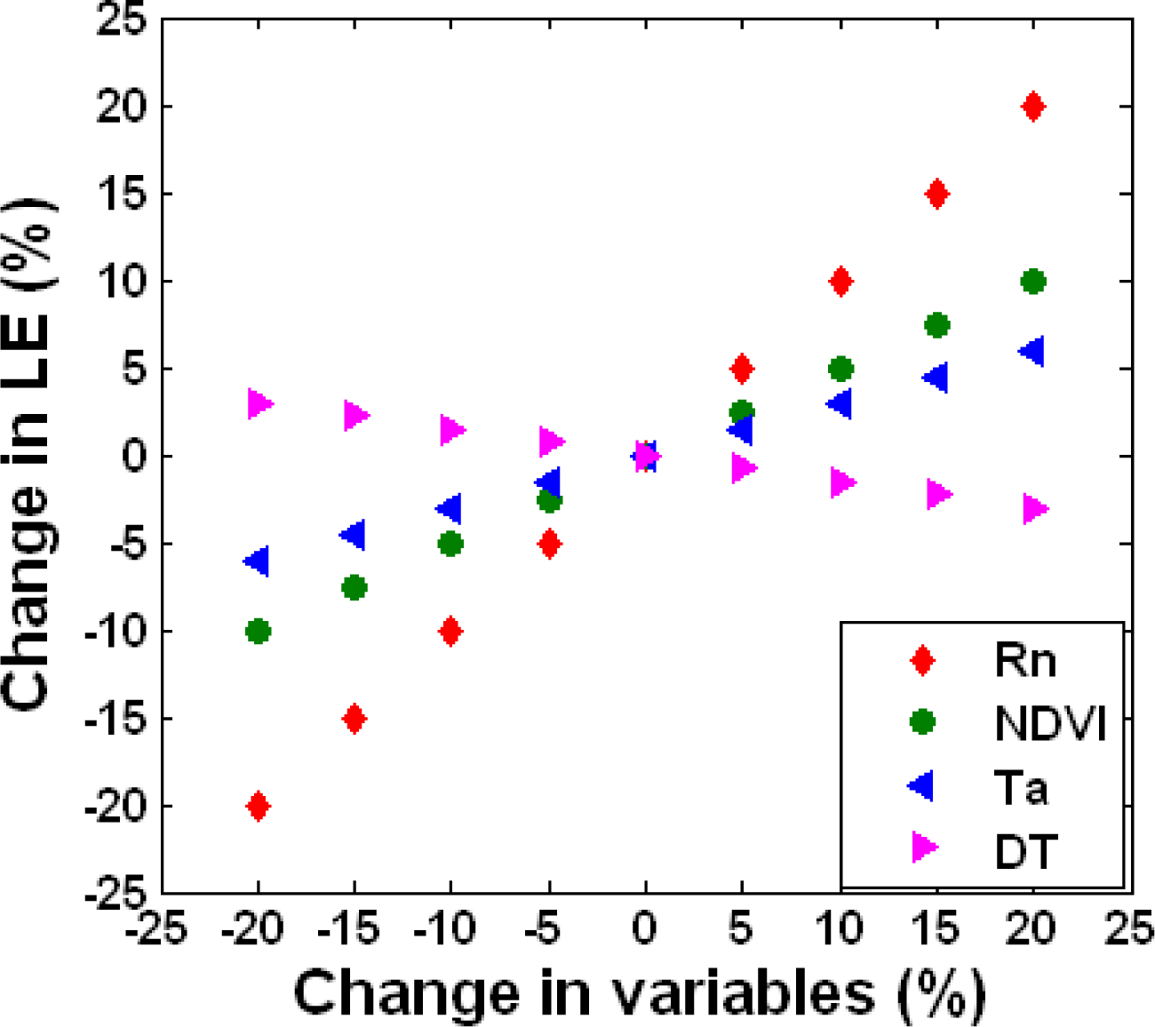
3.2. Sensitivity Analysis

To test the change in LE from the change in key input variables (Rn, NDVI, Ta and DT), sensitivity analysis of major parameters for the MS-PT algorithm is also conducted (Figure 6). As illustrated for the MS-PT algorithm, the largest change of LE is caused by the variation of Rn. Sensitivity of Rn is the highest in the MS-PT algorithm because the Priestley-Taylor equation is calculated as the sum of the surface energy balance term. The averaged LE varies at all flux towers up to ±20% for the MS-PT algorithm by changing Rn with ±20%. In response to the change in NDVI with ±20%, LE varies by ±10% at all flux towers. Similarly, LE can increase by 6% for Ta change of 20%. However, DT shows different sensitivity with the MS-PT algorithm and LE relatively increases up to 3% for DT change of −20%. Overall, LE estimation by the MS-PT algorithm shows the obvious sensitivity orders: Rn > NDVI > Ta > DT.
In the MS-PT algorithm proposed in this study, Rn acquires more highly dependent and this is generally consistent with the previous literature [58,59]. For example, Jang et al. [58] considered the sensitivity orders of estimated LE using satellite-based models with Rn (±12% change of LE for ±20% change of the variable) > LAI (approximate ±10%) > VPD and Ta (less than ±5%) at different land cover types. Hwang and Choi [59] found the sensitivity orders: Rn > LAI > Pa for the revised remote sensing-based PM model. Besides Rn, the Dependency of NDVI in the MS-PT algorithm is higher in the all flux towers as vegetation amount quantified by vegetation index (NDVI) and LAI affect the vegetation photosynthesis and transpiration [18,56]. Similarly, DT, reflecting the ATI, is an important factor controlling soil evaporation after surface soil moisture is deficient [60,61]. The variations of DT can lead to slight changes in soil evaporation. Compared with Rn, NDVI, and Ta, DT plays an insignificant role.

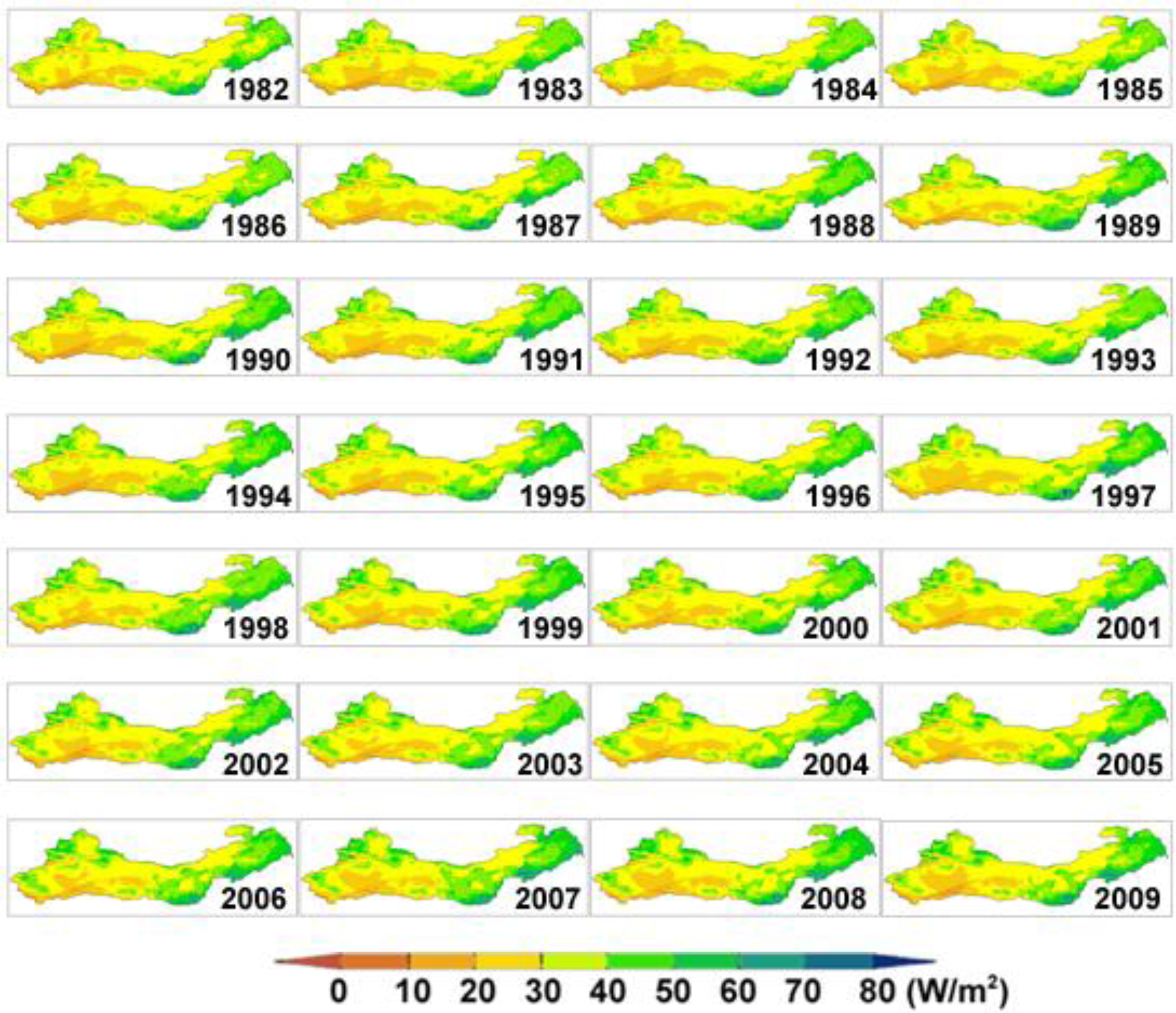
3.3. Application I: Mapping Terrestrial Evapotranspiration of the Three-North Shelter Forest Region of China

Three-North Shelter Forest Programme of China (TNSFP) is a large ecological restoration project aiming to restore and protect regional vegetation over northwestern, northern, and northeastern regions of China [62,63]. Three-North Shelter Forest Region of China (TNSFR) includes more than 550 Chinese counties and covers an area of 4,069,000 km2 mostly in arid and semi-arid regions [63]. Although great progress has been made to monitor the long-term variations of vegetation cover over TNSFR, better understanding of the degree of the variation of LE caused by increasing vegetation cover on decadal scales is still critical due to the deficiency of needed ground-observations data [6264].
To this end, the MS-PT algorithm driven by GMAO-MERRA and GIMMIS-NDVI products has been applied to generate monthly LE with at a 0.1-degree spatial resolution in this region during 1982–2009. Here, we do not directly use the GMAO-MERRA LE products as these products exist large uncertainty [5]. Figure 7 displays the map of annual composites of monthly LE for 1982–2009. The largest annual LE occurs in the boreal forest regions of Northeast China, followed by temperate regions of North China and the smallest LE occurs in the arid and semi-arid regions of Northwest China. The highest LE over Northeast China is closely linked to the higher forest cover and healthy forests can maintain long-term LE because forest roots can acquire moisture from deeper soil layers [5,21,45,46,65]. The higher LE over North China is mainly caused by large-scale crops. The lowest LE over Northwest China may be attributed to the fact that abnormal precipitation deficiency has raised the likelihood of increased droughts and reduced terrestrial LE.
Despite these general similarities for these annual LEs, slight inter-annual variability in spatial LE distributions does exist, driven mainly by differences in climate, hydrology, and vegetation status. Figure 8a demonstrates the spatial pattern of trend in annual LE over Three-North Shelter Forest Region of China. Overall, the actual LE has increased on average over the entire regions and the positive linear slope is about 0.15 W/m2 per year (p = 0.03) from 1982 through 2009. Regionally, the LE increased over large areas in both Northeast China and Northwest China (except for the Tarim Basin) while decreasing in both North China and the Tarim Basin. The variations of both air temperature and precipitation can explain these differences. In west arid and semi-arid regions, LE is dominated by the precipitation because most of the region is a precipitation-limited environment [5,66]. However, in east temperate regions, temperature plays a dominant role in controlling vegetation growth [5,21,67,68]. The rising temperature has prolonged the growing season to improve plant productivity and increased LE [63,69]. As shown in Figure 8, the spatial variation of the LE and the precipitation trends show the same general trends in west regions of China, while there are good agreement between the spatial variations of the LE and the air temperature trends in east regions of China. These spatial correspondences support the increasing air temperature in the East China and increasing precipitation in the West China, associated with climate warming during the past 30-year period, can be account for the variations of LE over Three-North Shelter Forest Region of China.

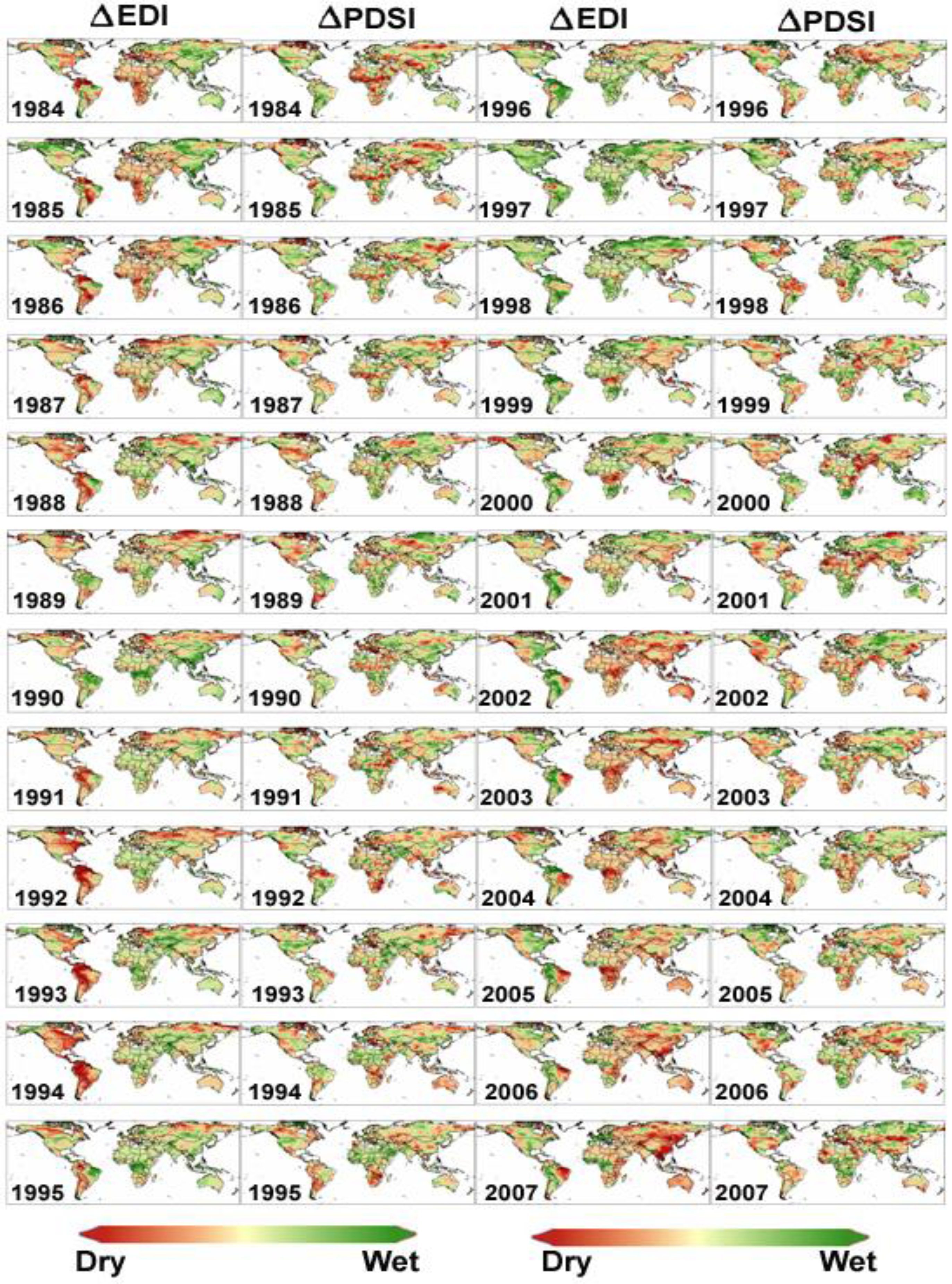
3.4. Application II: Monitoring Global Land Surface Drought

Drought is the most severe natural disaster causing global environmental changes and has attracted widespread attention from global scientists [70,71]. Recently, many satellite-based drought indices (e.g., Temperature-Vegetation Dryness Index, TVDI, and Evaporative Drought Index, EDI), have been widely used to monitor global or regional surface drought [4547,72,73]. Particularly for the LE-based EDI, it has integrated the actual LE and potential LE to isolate the effects due to spatially varying soil moisture availability, and has reflected a good correspondence with other meteorological drought indices, but at a significantly higher spatial resolution [32,4547,73].
To monitor long-term global surface drought, the MS-PT algorithm driven by GEWEX radiation products, NCEP-2 data, and GIMMIS-NDVI products has been applied to generate global monthly LE at a 1-degree spatial resolution during 1984–2007. GEWEX radiation products are used in this study as satellite-based radiation products are the main focus in global surface drought monitoring. Annual standardized anomalies in both EDI and PDSI from 1984 through 2007 are compared in Figure 9. Generally, the EDI successfully reproduces patterns evident in the PDSI, indicating the value of the satellite-derived NDVI and ATI signal as a surface moisture proxy. For example, MS-PT algorithm-based EDI captures the major global surface drought events occurring in 2000, 2002, 2003, 2005, and 2007, even in the Amazon Basin where there is dense vegetation cover and little exposure of the dry soil surface. Similarly, EDI also captures the wet events occurring in 1998 due to the last large El Niño event, which is consistent with the findings of other studies [21,24]. For instance, Jung et al. [24] reported that 1998 marks a transition period in which the global land LE trend decreases. The spatial pattern of trends in annual total EDI and PDSI from 1984 through 2007 has been examined (Figure 10). Substantial spatio-temporal variability appears in the dryness trends of EDI derived from GEWEX datasets that is almost consistent with that of PDSI. However, in the Eastern US, Western Australia, and the western regions of South America, the drought trend in EDI differs from the drought variability in PDSI. The missing and contaminated NDVI caused by cloud may lead to retrieval error in the EDI. Detailed speculations on the possible causes of this difference are challenging because drought is affected by variability in local atmospheric conditions (vapor pressure deficit, wind speed, air temperature, and relative humidity), moisture availability (precipitation), radiative forcing (cloud cover and sun angle), and vegetation amount.
Incorporating the optical remote sensing with a higher spatial resolution, we can produce daily time series required to calculate EDI at regional or field scales. For example, Yao et al. [47] generated daily EDI at 4-km resolution for April–September of 2003–2005 across the continental United States and found good performance of EDI in assessing drought at continental scales. These will facilitate drought assessment at field, regional and global scales, which will be valuable for drought monitoring and distribution of drought induced crop yield loss compensation.

4. Conclusions

We have presented a modified satellite-based Priestley-Taylor (MS-PT) algorithm to estimate terrestrial LE using remote sensing products and meteorological data. This algorithm is physically based, requiring no subjective parameter calibration as employed by many other traditional LE methods. We have also validated it using ground observations collected from 40 flux towers distributed across the world on all continents. The validations show that the RMSE of the estimated daily LE using MS-PT algorithm varies from 10.7 W/m2 to 87.6 W/m2, the bias varies from −23.7 W/m2 to 48.6 W/m2, and R2 varies from 0.41 to 0.89 (p < 0.01). Similarly, the RMSE of the estimated daily LE using PT-JPL algorithm varies from 11.3 W/m2 to 89.1 W/m2, the bias varies from −21.3 W/m2 to 56.2 W/m2, and R2 varies from 0.40 to 0.88 (p < 0.01). The average daily LE can be estimated reasonably in terms of the Root Mean Square Error and correlation coefficients. As compared with the PT-JPL algorithm, the MS-PT algorithm improves the LE estimates at most flux towers sites.
To evaluate how well the model predicts long-term variations in LE, we have validated the estimated annual LE anomalies with the observed annual LE anomalies. We only use flux tower sites where five years of data are available. The results illustrate that the bias of estimated annual LE anomalies deviating from ground-based observations is −2.3 W/m2, the RMSE is 11.2 W/m2 and R2 is 0.42 (p = 0.02). The MS-PT algorithm is also satisfactory in reproducing the inter-annual variability at sites with at least five years of data, indicating this method may be a good tool for analyzing the long-term variation of LE. The sensitivity analysis of major parameters for the MS-PT algorithm demonstrates that the sensitivity orders of estimated LE with Rn (±20% change of LE for ±20% change of the variable) > NDVI (approximate ± 10%) > Ta (±6%) and DT (±3%) for different land cover types.
This algorithm has been applied in mapping terrestrial LE of Three-North Shelter Forest Region of China and applied in monitoring global land surface drought. The decadal variation in LE of Three-North Shelter Forest region of China, during 1982–2009, illustrates that increasing air temperature in East China and increasing precipitation in West China, associated with climate warming during the past 30-year period, can explain the variations of LE over this region. Additionally, Evaporative Drought Index (EDI) has provided useful surface moisture proxy information without requiring precipitation data for global land surface drought monitoring. MS-PT algorithm-based EDI captures the major global surface drought events occurring in 2000, 2002, 2003, 2005, and 2007, even in the Amazon Basin where there is dense vegetation cover and little exposure of the dry soil surface. Similarly, EDI also captures the wet events occurring in 1998 due to the last large El Niño event, which is consistent with the findings of other studies. MS-PT algorithm-based EDI derived from optical remote sensing with a higher spatial resolution will facilitate drought assessment at field, regional and global scales, which will be valuable for drought monitoring and distribution of drought induced crop yield loss compensation.

Acknowledgments

Authors thank Xianglan Li, Liang Sun, Wenping Yuan, Xiaotong Zhang, Bo Jiang, Qiang Liu and Xiang Zhao from Beijing Normal University, China, for their suggestions. Authors would like to thank Yan Liu and Ran Li from Xinjiang Institute of Ecology and Geography, CAS, for providing ground-measured data. Latent heat flux, net radiation, shortwave solar radiation and corresponding meteorological observations were obtained from Asiaflux ( http://asiaflux.yonsei.kr/index.html), GAME AAN ( http://aan.suiri.tsukuba.ac.jp/), Ameriflux ( http://public.ornl.gov/ameriflux/index.html), the global FLUXNET project ( http://daac.ornl.gov/FLUXNET/fluxnet.html), ARM ( http://www.archive.arm.gov/), and the Global Energy and Water Cycle Experiment (GEWEX) Surface Radiation Budget (SRB) products ( http://gewex-srb.larc.nasa.gov/common/php/SRB_data_products.php). GIMMIS NDVI products were obtained from National Oceanic and Atmospheric Administration (NOAA)/AVHRR observations ( http://islscp2.sesda.com/ISLSCP21/data/vegetation/gimms_ndvi_monthly_xdeg/). Air temperature data were obtained from both NCEP/NCAR Reanalysis Project (CDAS) ( http://www.cpc.ncep.noaa.gov/products/wesley/reanalysis.html) and GMAO-MERRA ( http://disc.sci.gsfc.nasa.gov/daac-bin/FTPSubset.pl?LOOKUPID.List=MAIMCPASM). PDSI products were obtained the NCAR CGD’S Climate Analysis Section Palmer products ( http://www.cgd.ucar.edu/cas/catalog/climind/pdsi.html). This work was partially supported by the Natural Science Fund of China (No.41201331, No.41331173, No. 41230747 and No. 41101313), the National High Technology Research and Development Program of China (No. 2013AA121201), the Fundamental Research Funds for the Central Universities (No.2013YB34), the High Resolution Earth Observation Systems of National Science and Technology Major Projects (No.05-Y30B02-9001-13/15-9) and the National Science and Technology Support Plan During the 12th Five-year Plan Period of China (No.2012BAC19B03 and 2013BAC10B01).

Author Contributions

Yunjun Yao, Shunlin Liang and Shaohua Zhao prepared the manuscript. Yuhu Zhang, Qiming Qin, Jie Cheng and Kun Jia made the remote sensing images processing. Xianhong Xie, Nannan Zhang and Meng Liu contributed to the discussion.

Conflicts of Interest

The authors declare no conflict of interest.

References

  1. Trenberth, K.E.; Smith, L.; Qian, T.; Dai, A.; Fasullo, J. Estimates of the global water budget and its annual cycle using observational and model data. J. Hydrometeorol 2007, 8, 758–769. [Google Scholar]
  2. Wang, K.; Wang, P.; Li, Z.Q.; Cribb, M.; Sparrow, M. A simple method to estimate actual evapotranspiration from a combination of net radiation, vegetation index, and temperature. J. Geophys. Res 2007. [Google Scholar] [CrossRef]
  3. Li, Z.L.; Tang, R.L.; Wan, Z.M.; Bi, Y.Y.; Zhou, C.H.; Tang, B.H.; Yan, G.J.; Zhang, X.Y. A review of current methodologies for regional evapotranspiration estimation from remotely sensed data. Sensors 2009, 9, 3801–3853. [Google Scholar]
  4. Liang, S.; Wang, K.; Zhang, X.; Wild, M. Review on estimation of land surface radiation and energy budgets from ground measurements, remote sensing and model simulations. IEEE J. Sel. Top. Appl. Earth Observ. Remote Sens 2010, 3, 225–240. [Google Scholar]
  5. Wang, K.; Dickinson, R. A review of global terrestrial evapotranspiration: Observation, modeling, climatology and climatic variability. Rev. Geophys 2012. [Google Scholar] [CrossRef]
  6. Stisen, S.; Sandholt, I.; Nørgaard, A.; Fensholt, R.; Jensen, K.H. Combining the triangle method with thermal inertia to estimate regional evapotranspiration—Applied to MSGSEVIRI data in the Senegal River basin. Remote Sens. Environ 2008, 112, 1242–1255. [Google Scholar]
  7. Zhang, K.; Kimball, J.S.; Mu, Q.; Jones, L.A.; Goetz, S.J.; Running, S.W. Satellite based analysis of northern ET trends and associated changes in the regional water balance from 1983 to 2005. J. Hydrol 2009, 379, 92–110. [Google Scholar]
  8. Zhang, K.; Kimball, J.S.; Nemani, R.R.; Running, S.W. A continuous satellite-derived global record of land surface evapotranspiration from 1983 to 2006. Water Resour. Res 2010. [Google Scholar] [CrossRef]
  9. Yuan, W.; Liu, S.; Yu, G.; Bonnefond, J.M.; Chen, J.; Davis, K.; Desai, A.R.; Goldstein, A.H.; Gianelle, D.; Rossi, F.; et al. Global estimates of evapotranspiration and gross primary production based on MODIS and global meteorology data. Remote Sens. Environ 2010, 114, 1416–1431. [Google Scholar]
  10. Yao, Y.; Qin, Q.; Ghulam, A.; Liu, S.; Zhao, S.; Xu, Z.; Dong, H. Simple method to determine the Priestley-Taylor parameter for evapotranspiration estimation using Albedo-VI triangular space from MODIS data. J. Appl. Remote Sens 2011. [Google Scholar] [CrossRef]
  11. Norman, J.M.; Kustas, W.P.; Humes, K.S. A two-source approach for estimating soil and vegetation energy fluxes in observations of directional radiometric surface temperature. Agric. For. Meteorol 1995, 77, 263–293. [Google Scholar]
  12. Kustas, W.P.; Norman, J.M. Use of remote sensing for evapotranspiration monitoring over land surfaces. Hydrol. Sci. J 1996, 41, 495–516. [Google Scholar]
  13. Anderson, M.C.; Norman, J.M.; Diak, G.R.; Kustas, W.P.; Mecikalski, J.R. A two-source time-integrated model for estimating surface fluxes using thermal infrared remote sensing. Remote Sens. Environ 1997, 60, 195–116. [Google Scholar]
  14. Cleugh, H.A.; Leuning, R.; Mu, Q.; Running, S.W. Regional evaporation estimates from flux tower and MODIS satellite data. Remote Sens. Environ 2007, 106, 285–304. [Google Scholar]
  15. Mu, Q.; Heinsch, F.A.; Zhao, M.; Running, S.W. Development of a global evapotranspiration algorithm based on MODIS and global meteorology data. Remote Sens. Environ 2007, 111, 519–536. [Google Scholar]
  16. Mu, Q.; Zhao, M.; Running, S.W. Improvements to a MODIS global terrestrial evapotrans piration algorithm. Remote Sens. Environ 2011, 115, 1781–1800. [Google Scholar]
  17. Fisher, J.; Tu, K.; Baldocchi, D. Global estimates of the land atmosphere water flux based on monthly AVHRR and ISLSCP-II data, validated at 16 FLUXNET sites. Remote Sens. Environ 2008, 112, 901–919. [Google Scholar]
  18. Wang, K.; Liang, S. An improved method for estimating global evapotranspiration based on satellite determination of surface net radiation, vegetation index, temperature, and soil moisture. J. Hydrometeorol 2008, 9, 712–727. [Google Scholar]
  19. Wang, K.; Dickinson, R.; Wild, M.; Liang, S. Evidence for decadal variation in global terrestrial evapotranspiration between 1982 and 2002. Part 1: Model development. J. Geophys. Res 2010. [Google Scholar] [CrossRef]
  20. Wang, K.; Dickinson, R.; Wild, M.; Liang, S. Evidence for decadal variation in global terrestrial evapotranspiration between 1982 and 2002. Part 2: Results. J. Geophys. Res 2010. [Google Scholar] [CrossRef]
  21. Yao, Y.; Liang, S.; Cheng, J.; Liu, S.; Fisher, J.; Zhang, X.; Jia, K.; Zhao, X.; Qin, Q.; Zhao, B.; et al. MODIS-driven estimation of terrestrial latent heat flux in China based on a modified Priestley-Taylor algorithm. Agric. For. Meteorol 2013, (171–172), 187–202. [Google Scholar]
  22. Kalma, J.; McVicar, T.; McCabe, M. Estimating land surface evaporation: A review of methods using remotely sensed surface temperature data accomplished. Surv. Geophys 2008, 29, 421–469. [Google Scholar]
  23. Jackson, R.; Reginato, R.; Idso, S. Wheat canopy temperature: A practical tool for evaluating water requirements. Water Resour. Res 1977, 13, 651–656. [Google Scholar]
  24. Jung, M.; Reichstein, M.; Ciais, P.; Seneviratne, S.; Sheffield, J.; Goulden, M.; Bonan, G.; Cescatti, A.; Chen, J.; Richard, D.; et al. Recent decline in the global land evapotranspiration trend due to limited moisture supply. Nature 2010, 467, 951–954. [Google Scholar]
  25. Boegh, E.; Soegaard, H.; Hanan, N.; Kabat, P.; Lesch, L. A remote sensing study of the NDVI–Ts relationship and the transpiration from sparse vegetation in the Sahel based on high-resolution satellite data. Remote Sens. Environ 1999, 69, 224–240. [Google Scholar]
  26. Shuttleworth, W.J.; Wallace, J.S. Evaporation from sparse crops an energy combination theory. Quart. J. R. Meteorol. Soc 1985, 111, 839–855. [Google Scholar]
  27. Monteith, J. Evaporation and environment. Symp. Soc. Exp. Biol 1965, 19, 205–224. [Google Scholar]
  28. Boni, G.; Entekhabi, D.; Castelli, F. Land data assimilation with satellite measurements for the estimation of surface energy balance components and surface control on evaporation. Water Resour. Res 2001, 37, 1713–1722. [Google Scholar]
  29. Qin, J.; Liang, S.; Liu, R.; Zhang, H.; Hu, B. A weak-constraint based data assimilation scheme for estimating surface turbulent fluxes. IEEE Geosci. Remote Sens 2007, 4, 649–653. [Google Scholar]
  30. Pipunic, R.; Walker, J.; Western, A. Assimilation of remotely sensed data for improved latent and sensible heat flux prediction: A comparative synthetic study. Remote Sens. Environ 2008, 112, 1295–1305. [Google Scholar]
  31. Jiang, L.; Islam, S. Estimation of surface evaporation map over Southern Great Plains using remote sensing data. Water Resour. Res 2001, 37, 329–340. [Google Scholar]
  32. Yao, Y.; Liang, S.; Qin, Q.; Wang, K.; Zhao, S. Monitoring global land surface drought based on a hybrid evapotranspiration model. Int. J. Appl. Earth Observ 2011, 13, 447–457. [Google Scholar]
  33. Priestley, C.H.B.; Taylor, R.J. On the assessment of surface heat flux and evaporation using large-scale parameters. Mon. Weath. Rev 1972, 100, 81–92. [Google Scholar]
  34. Jin, Y.; Randerson, J.; Goulden, M. Continental-scale net radiation and evapotranspiration estimated using MODIS satellite observations. Remote Sens. Environ 2011, 115, 2302–2319. [Google Scholar]
  35. Miralles, D.G.; Holmes, T.R.H.; de Jeu1, R.A.M.; Gash, G.H.; Meesters, A.G.C.A.; Dolman, A.J. Global land-surface evaporation estimated from satellite-based observations. Hydrol. Earth Syst. Sci 2011, 15, 453–469. [Google Scholar]
  36. Mueller, B.; Seneviratne, S.I.; Jimenez, C.; Corti, T.; Hirschi, M.; Balsamo, G.; Ciais, P.; Dirmeyer, P.; Fisher, J.; Guo, Z.; et al. Evaluation of global observations-based evapotranspiration datasets and IPCC AR4 simulations. Geophys. Res. Lett 2011. [Google Scholar] [CrossRef]
  37. Jiang, L.; Islam, S.; Guo, W.; Jutla, A.S.; Senarath, S.U.S.; Ramsay, B.H.; Eltahir, E. A satellite-based daily actual evapotranspiration estimation algorithm over South Florida. Glob. Planet. Chang 2009, 67, 62–77. [Google Scholar]
  38. Nemani, R.R.; Keeling, C.D.; Hashimoto, H.; Jolly, W.M.; Piper, S.C.; Tucker, C.J.; Myneni, R.B.; Running, S.W. Climate-driven increases in global terrestrial net primary production from 1982 to 1999. Science 2003, 300, 1560–1563. [Google Scholar]
  39. Jiang, L.; Islam, S. A methodology for estimation of surface evapotranspiration over large areas using remote sensing observations. Geophys. Res. Lett 1999, 26, 2773–2776. [Google Scholar]
  40. Wang, K.; Li, Z.; Cribb, M. Estimation of evaporative fraction from a combination of day and night land surface temperatures and NDVI: A new method to determine the Priestley-Taylor parameter. Remote Sens. Environ 2006, 102, 293–305. [Google Scholar]
  41. Carlson, T. An overview of the “Triangle Method” for estimating surface evapotranspiration and soil moisture from satellite imagery. Sensors 2007, 7, 1612–1629. [Google Scholar]
  42. Tang, R.; Li, Z.; Tang, B. An application of the Ts-VI triangle method with enhanced edges determination for evapotranspiration estimation from MODIS data in arid and semi-arid regions: Implementation and validation. Remote Sens. Environ 2010, 114, 540–551. [Google Scholar]
  43. Anderson, M.C.; Kustas, W.P.; Norman, J.M.; Hain, C.R.; Mecikalski, J.R.; Schultz, Z.; González-Dugo, M.P.; Cammalleri, C.; D’Urso, G.; Pimstein, A.; et al. Mapping daily evapotranspiration at field to continental scales using geostationary and polar orbiting satellite imagery. Hydrol. Earth Syst. Sci 2011, 15, 223–239. [Google Scholar] [Green Version]
  44. Yebra, M.; Dijk, A.V.; Leuning, R.; Huete, A.; Guerschman, J.P. Evaluation of optical remote sensing to estimate actual evapotranspiration and canopy conductance. Remote Sens. Environ 2013, 129, 250–261. [Google Scholar]
  45. Anderson, M.C.; Norman, J.M.; Mecikalski, J.R.; Otkin, J.A.; Kustas, W.P. A climatological study of evapotranspiration and moisture stress across the continental United States based on thermal remote sensing: 1. Model formulation. J. Geophys. Res 2007. [Google Scholar] [CrossRef]
  46. Anderson, M.C.; Norman, J.M.; Mecikalski, J.R.; Otkin, J.A.; Kustas, W.P. A climatological study of evapotranspiration and moisture stress across the continental United States based on thermal remote sensing: 2. Surface moisture climatology. J. Geophys. Res 2007. [Google Scholar] [CrossRef]
  47. Yao, Y.; Liang, S.; Qin, Q.; Wang, K. Monitoring drought over the conterminous united states using MODIS and NCEP reanalysis-2 data. J. Meteor. Appl. Climatol 2010, 49, 1665–1680. [Google Scholar]
  48. Hargreaves, G.H. Defining and using reference evapotranspiration. J. Irrig. Drain. Eng 1994, 120, 1132–1139. [Google Scholar]
  49. Pinker, R.T.; Zhang, B.; Dutton, E.G. Do satellites detect trends in surface solar radiation? Science 2005, 308, 850–854. [Google Scholar]
  50. Twine, T.E.; Kustas, W.P.; Norman, J.M.; Cook, D.R.; Houser, P.R.; Meyers, T.P.; Prueger, J.H.; Starks, P.J.; Wesely, M.L. Correcting eddy-covariance flux underestimates over a grassland. Agric. For. Meteorol 2000, 103, 279–300. [Google Scholar]
  51. Tucker, C.J.; Pinzon, J.E.; Brown, M.E.; Slayback, D.A.; Pak, E.W.; Mahoney, R.; Vermote, E.F.; Saleous, N. An extended AVHRR 8-km NDVI dataset compatible with MODIS and SPOT vegetation NDVI data. Int. J. Remote Sens 2005, 26, 4485–4498. [Google Scholar]
  52. Wu, J.B.; Xiao, X.M.; Guan, D.X.; Shi, T.T.; Jin, C.J.; Han, S.J. Estimation of the gross primary production of an old-growth temperate mixed forest using eddy covariance and remote sensing. Int. J. Remote Sens 2009, 30, 463–479. [Google Scholar]
  53. Wang, H.S.; Jia, G.S.; Fu, C.B.; Feng, J.M.; Zhao, T.B.; Ma, Z.G. Deriving maximal light use efficiency from coordinated flux measurements and satellite data for regional gross primary production modeling. Remote Sens. Environ 2010, 114, 2248–2258. [Google Scholar]
  54. Glenn, E.P.; Huete, A.R.; Nagler, P.L.; Nelson, S.G. Relationship between remotely-sensed vegetation indices, canopy attributes and plant physiological processes: What vegetation indices can and cannot tell us about the landscape. Sensors 2008, 8, 2136–2160. [Google Scholar]
  55. Zeng, X.B.; Dickinson, R.E.; Walker, A.; Shaikh, M.; DeFries, R.S.; Qi, J.G. Derivation and evaluation of global 1-km fractional vegetation cover data for land modeling. J. Appl. Meteorol 2000, 39, 826–839. [Google Scholar]
  56. Tucker, C.J. Red and photographic infrared linear combinations for monitoring. Remote Sens. Environ 1979, 8, 127–150. [Google Scholar]
  57. Li, R.; Min, Q.L.; Lin, B. Estimation of evapotranspiration in a mid-latitude forest using the microwave emissivity difference vegetation index (EDVI). Remote Sens. Environ 2009, 113, 2011–2018. [Google Scholar]
  58. Jang, K.; Kang, S.; Kim, J.; Lee, C.B.; Kim, T.; Kim, J.; Hirata, R.; Saigusa, N. Mapping evapotranspiration using MODIS and MM5 four-dimensional data assimilation. Remote Sens. Environ 2010, 114, 657–673. [Google Scholar]
  59. Hwang, K.; Choi, M. Seasonal trends of satellite-based evapotranspiration algorithms over a complex ecosystem in East Asia. Remote Sens. Environ 2013, 137, 244–263. [Google Scholar]
  60. Salvucci, G.D. Soil and moisture independent estimation of stage-two evaporation from potential evaporation and albedo or surface temperature. Water Resour. Res 1997, 33, 111–122. [Google Scholar]
  61. Gu, L.; Meyers, T.; Pallardy, S.G.; Hanson, P.J.; Yang, B.; Heuer, M.; Hosman, K.P.; Riggs, J.S.; Sluss, D.; Wullschleger, S.D. Direct and indirect effects of atmospheric conditions and soil moisture on surface energy partitioning revealed by a prolonged drought at a temperate forest site. J. Geophys. Res 2006. [Google Scholar] [CrossRef]
  62. Wu, Y.; Zeng, Y.; Wu, B. Retrieval and analysis of vegetation cover in the Three-North Regions of China based on MODIS data. Chin. J. Ecol 2009, 28, 1712–1718. [Google Scholar]
  63. Duan, H.; Yan, C.; Tsunekawa, A.; Song, X.; Li, S.; Xie, J. Assessing vegetation dynamics in the Three-North Shelter Forest region of China using AVHRR NDVI data. Environ. Earth Sci 2011, 64, 1011–1020. [Google Scholar]
  64. Li, S.; Zhai, H. The comparison study on forestry ecological projects in the world (In Chinese). Acta. Ecol. Sin 2002, 22, 1976–1982. [Google Scholar]
  65. Yao, Y.; Liang, S.; Qin, Q.; Wang, K.; Liu, S.; Zhao, S. Satellite detection of increases in global land surface evapotranspiration during 1984–2007. Int. J. Digit. Earth 2012, 5, 299–318. [Google Scholar]
  66. Lu, E.; Luo, Y.L.; Zhang, R.H.; Wu, Q.X.; Liu, L.P. Regional atmospheric anomalies responsible for the 2009–2010 severe drought in China. J. Geophys. Res 2011. [Google Scholar] [CrossRef]
  67. Myneni, R.B.; Yang, W.; Nemani, R.R.; Huete, A.R.; Dickinson, R.E.; Knyazikhin, Y.; Didan, K.; Fu, R.; Negron Juarez, R.I.; Saatchi, S.S.; et al. Large seasonal swings in leaf area of Amazon rainforests. Proc. Natl. Acad. Sci. USA 2007, 104, 4820–4823. [Google Scholar]
  68. Sasai, T.; Saigusa, N.; Nasahara, K.N.; Ito, A.; Hashimoto, H.; Nemani, R.; Hirata, R.; Ichii, K.; Takagi, K.; Saitoh, T.M.; et al. Satellite-driven estimation of terrestrial carbon flux over Far East Asia with 1-km grid resolution. Remote Sens. Environ 2011, 115, 1758–1771. [Google Scholar]
  69. Zhao, M.; Running, S.W. Drought-induced reduction in global terrestrial net primary production from 2000 through 2009. Science 2010, 329, 940–943. [Google Scholar]
  70. Dai, A.G.; Trenberth, K.E.; Qian, T. A global data set of Palmer Drought Severity Index for 1870–2002: Relationship with soil moisture and effects of surface warming. J. Hydrometeorol 2004, 5, 1117–1130. [Google Scholar]
  71. Robeson, S.M. Applied climatology: Drought. Progr. Phys. Geogr 2008, 32, 303–309. [Google Scholar]
  72. Sandholt, I.; Rasmussen, K.; Andersen, J. A simple interpretation of the surface temperature-vegetation index space for assessment of surface moisture status. Remote Sens. Environ 2002, 79, 213–224. [Google Scholar]
  73. Mu, Q.; Zhao, M.; Kimball, J.S.; McDowell, N.G.; Running, S.W. A remotely sensed global terrestrial drought severity index. Bull. Am. Meteor. Soc 2013, 94, 83–97. [Google Scholar]
Figure 1. Schematic diagram of the modified satellite-based Priestley-Taylor model (“Tree” picture source derived from Anderson et al. [45]).
Remotesensing 06 00880f1
Figure 2. Location of the 40 flux tower sites used in this study.
Remotesensing 06 00880f2
Figure 3. Eight-day time series comparisons of the modeled LE (daily total) estimates based on two PT algorithms and the ground-measured LE using the data collected from the ten flux towers in their respective land cover classes from the validation tower set. DBF: deciduous broadleaf forest; DNF: Deciduous needleleaf forest; EBF: evergreen broadleaf forest; ENF: evergreen needleleaf forest; MF: mixed forest; SHR: shrubland. All r values are significant with 99% confidence.
Remotesensing 06 00880f3
Figure 4. Comparison of the predicted and ground-measured annual LE collected at all 40 flux towers sites shown in Table 1.
Remotesensing 06 00880f4
Figure 5. Comparison of the annual anomalies of predicted LE and ground-measured LE collected at the flux towers sites where at least five years of data are available.
Remotesensing 06 00880f5
Figure 6. Sensitivity analysis of LE with net radiation, NDVI, DT, and air pressure near surface.
Remotesensing 06 00880f6
Figure 7. Map of annual composites of monthly LE over Three-North Shelter Forest Region of China for 1982–2009.
Remotesensing 06 00880f7
Figure 8. Spatial pattern of linear trends in annual (a) LE based on MS-PT algorithm driven by GMAO-MERRA data and GIMMIS-NDVI products; (b) Precipitation from GMAO-MERRA data; and (c) air temperature from GMAO-MERRA data during 1982–2009.
Remotesensing 06 00880f8
Figure 9. Annual anomalies in global land surface EDI and PDSI for 1984–2007.
Remotesensing 06 00880f9
Figure 10. Spatial pattern of linear trends in annual (a) EDI and (b) PDSI, from 1984 through 2007.
Remotesensing 06 00880f10
Table 1. A description of site conditions. Land cover types, Latitude (Lat), longitude (Lon), Elevation (Elev, meter), time-period, and network names are shown here.
Site NameCountryLand Cover TypesLatLonElevTime PeriodNetwork
Sask-Fire 1977 (CA-SF1)CanadaEvergreen needleleaf forest54.49−105.825362003–2005FLUXNET
UCI-1850 burn site (CA-NS1)CanadaEvergreen needleleaf forest55.88−98.482602002–2005AmeriFlux
Quebec Mature Boreal Forest Site (CA-Qfo)CanadaEvergreen needleleaf forest49.69−74.343822003–2006FLUXNET
Ivotuk (US-Ivo)USAOpen shrubland68.49−155.755682003–2006AmeriFlux
Metolius-old aged ponderosa pine (US-Me4)USAEvergreen needleleaf forest44.50−121.629222000AmeriFlux
ARM Southern Great Plains site-Lamont (US-ARM)USACentral facility tower crop field36.61−97.493142003–2006AmeriFlux
Audubon Research Ranch (US-Aud)USAGrassland31.59−110.511,4692002–2006AmeriFlux
Mead--irrigated continuous maize site (US-Ne1)USACropland41.17−96.483612001–2005AmeriFlux
Morgan Monroe State Forest (US-MMS)USADeciduous broadleaf forest39.32−86.412752000–2005AmeriFlux
Slashpine-Austin Cary-65y nat regen (US-Sp1)USAEvergreen needleleaf forest29.74−82.22502000–2005AmeriFlux
Howland Forest (US-Ho1)USAClosed conifer forest45.20−68.74602000–2004AmeriFlux
Santarem-Km83-Logged Forest (BR-Sa3)BrazilCleared forest−3.02−54.971002000–2003AmeriFlux
Maun-Mopane Woodland (BW-Ma1)BotswanaSavanna woodland−19.9223.569502000–2001FLUXNET
Ghanzi Mixed Site (BW-Ghm)BotswanaWoody savanna−21.221.751,1352003FLUXNET
Skukuza-Kruger National Park (ZA-Kru)South AfricaSavanna−25.0231.503652001–2003FLUXNET
Niamey (NI-Nam)NigerOpen shrubland13.482.182232006ARM
Yatir (IL-Yat)IsraelEvergreen needleleaf forest31.3535.056502001–2006FLUXNET
Palangkaraya (ID-Pag)IndonesiaEvergreen broadleaf forest2.35114.04302002–2003AsiaFlux
CocoFlux (VU-Coc)VanuatuEvergreen broadleaf forest−15.44167.19802001–2004FLUXNET
Mae Klong (TH-Mkl)ThailandMixed deciduous forest14.5898.842312003–2004AsiaFlux
Howard Springs (AU-How)AustraliaWoody savanna−12.49131.1552001–2006FLUXNET
Tumbarumba (AU-Tum)AustraliaEvergreen broadleaf forest−35.66148.151,2002001–2006FLUXNET
Wallaby Creek (AU-Wac)AustraliaEvergreen broadleaf forest−37.43145.195452005–2007FLUXNET
Tomakomai Flux Research Site (JP-Tmk)JapanJapanese larch forest42.74141.521402001–2003AsiaFlux
Arvaikheer (MN-Arv)MongoliaGrassland46.23102.831,7282000–2003GAME AAN
Southern Khentei Taiga (MN-Skt)MongoliaLarch forest48.35108.651,6302003–2006AsiaFlux
Fukang (CN-Fuk)ChinaGrassland44.2887.924762006–2007CERN
Zotino (RU-Zot)RussiaEvergreen needleleaf forest60.8089.35902002–2004FLUXNET
Siberia Yakutsk Larch Forest Site (RU-Ylf)RussiaLarch forest62.26129.242202003–2004AsiaFlux
Chokurdakh (RU-Cok)RussiaOpen shrubland70.62147.88232003–2005FLUXNET
Fyodorovskoye wet spruce stand (RU-Fyo)RussiaSpruce forest56.4632.922652000–2006FLUXNET
Kaamanen wetland (FI-Kaa)FinlandWetlands69.1427.301552000–2006FLUXNET
Fajemyr (SE-Faj)SwedenWetlands56.2713.551402005–2006FLUXNET
Polwet (PL-Wet)PolandWetlands52.7616.31542004–2005FLUXNET
Neustift/Stubai Valley (AT-Neu)AustriaGrassland47.1211.329702002–2006FLUXNET
Amplero (IT-Amp)ItalyGrassland41.9013.618842002–2006FLUXNET
Las Majadas del Tietar (ES-Lma)SpainSavanna39.94−5.772602004–2006FLUXNET
Griffin-Aberfeldy-Scotland (UK-Gri)UKEvergreen needleleaf forest56.61−3.803402000–2006FLUXNET
Tatra (SK-Tat)Slovak RepublicEvergreen needleleaf forest49.1220.161,0502005FLUXNET
Foulum (DK-Fou)DenmarkCropland56.489.59512005FLUXNET
Tharandt (DE-Tha)GermanyNorway Spruce50.9713.573802000–2006FLUXNET
Table 2. Statistics of estimated daily LE against the eddy-flux tower observations. The bias and Root Mean Square Error (RMSE) are in units of W/m2. All r values are significant with 99% confidence.
Site NameBias (W/m2)RMSE (W/m2)R2

MS-PTPT-JPLMS-PTPT-JPLMS-PTPT-JPL
CA-SF1−13.512.726.835.30.890.87
CA-NS122.736.850.368.60.740.66
CA-Qfo6.8−4.736.140.10.710.51
US-Ivo−7.73.929.336.10.530.54
US-Me44.612.341.162.20.750.78
US-ARM−13.1−3.643.139.80.600.62
US-Aud−0.43.534.128.80.640.73
US-Ne1−13.6−5.745.654.10.870.78
US-MMS25.321.842.449.60.890.87
US-Sp146.356.260.281.30.850.81
US-Ho132.235.856.363.50.830.78
BR-Sa310.417.829.639.10.880.87
BW-Ma112.820.537.946.70.620.58
BW-Ghm−9.118.438.741.60.770.73
ZA-Kru−14.8−1.136.817.80.450.50
NI-Nam26.431.346.250.10.540.61
IL-Yat48.643.787.689.10.410.40
ID-Pag14.321.242.750.40.700.68
VU-Coc34.332.157.662.50.890.85
TH-Mkl21.628.947.767.80.670.61
AU-How13.523.944.361.80.700.64
AU-Tum10.926.234.156.60.880.84
AU-Wac22.528.847.461.10.850.80
JP-Tmk2.610.244.751.40.710.66
MN-Arv−20.4−12.558.741.60.440.54
MN-Skt20.126.141.646.50.720.69
CN-Fuk10.115.139.943.10.530.51
RU-Zot9.318.228.244.30.780.73
RU-Ylf−0.34.310.711.30.560.60
RU-Cok−12.3−1.328.549.10.720.62
RU-Fyo19.120.853.353.80.800.75
FI-Kaa−18.2−12.432.529.80.770.76
SE-Faj15.222.244.466.40.830.67
PL-Wet−23.7−11.337.529.40.890.85
AT-Neu−20.2−10.239.531.80.880.88
IT-Amp−23.1−11.548.342.50.710.72
ES-Lma−9.96.932.834.20.610.61
UK-Gri−21.7−21.342.343.20.760.74
SK-Tat−0.5−13.512.530.20.810.72
DK-Fou14.618.753.566.90.410.40
DE-Tha22.720.459.258.80.760.71

