The Uncertainty of Plot-Scale Forest Height Estimates from Complementary Spaceborne Observations in the Taiga-Tundra Ecotone

Abstract
: Satellite-based estimates of vegetation structure capture broad-scale vegetation characteristics as well as differences in vegetation structure at plot-scales. Active remote sensing from laser altimetry and radar systems is regularly used to measure vegetation height and infer vegetation structural attributes, however, the current uncertainty of their spaceborne measurements is likely to mask actual plot-scale differences in vertical structures in sparse forests. In the taiga (boreal forest)–tundra ecotone (TTE) the accumulated effect of subtle plot-scale differences in vegetation height across broad-scales may be significant. This paper examines the uncertainty of plot-scale forest canopy height measurements in northern Siberia Larix stands by combining complementary canopy surface elevations derived from satellite photogrammetry and ground elevations derived from the Geosciences Laser Altimeter System (GLAS) from the ICESat-1 satellite. With a linear model, spaceborne-derived canopy height measurements at the plot-scale predicted TTE stand height ∼5 m–∼10 m tall (R2 = 0.55, bootstrapped 95% confidence interval of R2 = 0.36–0.74) with an uncertainty ranging from ±0.86 m–1.37 m. A larger sample may mitigate the broad uncertainty of the model fit, however, the methodology provides a means for capturing plot-scale canopy height and its uncertainty from spaceborne data at GLAS footprints in sparse TTE forests and may serve as a basis for scaling up plot-level TTE vegetation height measurements to forest patches.1. Introduction
Boreal vegetation structure is an important factor in the arctic climate system [1,2]. Satellite-based estimates of vegetation structure capture broad-scale (e.g., across ecoregions) vegetation characteristics and as well as differences in vegetation structure at plot- or site-scales (e.g., ∼100 m2–1 ha), which have a direct effect on ecosystem processes. The taiga-tundra ecotone (TTE) at the convergence of the boreal forest and un-forested tundra has heterogeneous tree cover, and has seen recent widespread, yet variable, changes in vegetation structure [3–7]. Vegetation structural attributes, such as height, may influence ground temperatures, active-layer depth, albedo, and atmospheric warming [8–14]. The TTE is also variable in its response to environmental change, likely a result of interacting environmental factors including substrate, disturbance history, and geographic position [15–17].
TTE vegetation height is neither spatially uniform in its current state nor in the manner in which it is changing [18]. Spaceborne remote sensing that provides a synoptic perspective of certain plot-level details may help improve understanding of the net effect of these feedbacks on the climate system and the relative control from site factors [9,19]. The synoptic yet detailed perspective of plot-level vegetation characteristics and spatial arrangement derived from high-resolution (<5 m) spaceborne remote sensing (e.g., Worldview-1, -2, -3, GeoEye-1, and IKONOS) may help resolve observed disagreement between coarse-scale remote sensing results and plot-level characteristics in a systematic manner [6,20].
Vegetation structure, including forest height, has been estimated from a variety of spaceborne sensors at a range of scales [21–34]. The direct measurements of structure from active remote sensing from light detection and ranging (LiDAR) and synthetic aperture radar (SAR) continue to be regularly used to estimate vegetation height and infer structural attributes across a range of vegetation types. Often, spaceborne data has been coupled with airborne LiDAR surveys to link ground inventories with satellite measurements [26,35–37]. However, large portions of the TTE are difficult to access because they are remote and often require an airborne inventory involving multi-national cooperation. As such, the availability of the airborne component of remote vegetation structure measurements in the TTE is highly irregular. At this point, the systematic sampling available across the entire TTE offered by spaceborne instruments will likely yield the only comprehensive remote vegetation estimates.
Spaceborne estimates from SAR and LiDAR at the plot-scale in the TTE, however, have errors of inferred structure (above-ground biomass density) that are uncertain and relatively large (∼50%) [38]. Spaceborne SAR sensors estimate plot-level vegetation structure with high uncertainty due to the need to average many contiguous radar pixels, which causes conflicts of scale with ground data [39]. Spaceborne LiDAR from the Geoscience Laser Altimeter System (GLAS) on the ICESat-1 satellite has difficulty capturing canopy surface in sparse and short stature forests [40]. In the TTE, the uncertainty of these measurements alone may mask subtle yet significant plot-level vegetation height differences (e.g., 0.5 m–4 m) that may play a central role in the prediction of climate feedbacks in the high northern latitudes [9,41].
High resolution spaceborne imagery (HRSI) is increasingly being used for understanding detailed vegetation structural characteristics [42–44], particularly vegetation height [45–49]. More work into the use of HRSI for deriving vegetation heights in the TTE is warranted given their ability to resolve individual trees and tree shadows, their stereo viewing capabilities, and the importance of vegetation height on biophysical processes in the Arctic. With mounting HRSI data volumes, there is an increased opportunity to exploit the most useful characteristics of these data to refine spaceborne measurements of vegetation structure [50].
The availability of a variety of vegetation observations provides an opportunity to explore how these data complement each other to reduce uncertainty in measurements of vegetation characteristics. Complementary datasets may be those whose best observations depict different characteristics and, when combined, can provide a single measurement that would otherwise be unavailable with one dataset alone. Observations of current vegetation may be improved with archival or legacy data from different sensors acquired at different times, to derive vegetation structure characteristics. These applications and measurements could be useful for a broad spectrum of spatial scientists [51] if the uncertainty associated with the measurements is well-documented.
An example of complementary satellite measurements of TTE vegetation structure may come from GLAS LiDAR and Worldview-1. Each make a direct and unique measurement of surface features that can provide information on vegetation structure [52,53]. The spatial resolution of these measurements (50–60 m major axis for the elliptical GLAS footprint; ∼0.5 m pixel size for HRSI from Worldview-1) are at scales well suited for comparison with field plot measurements that typically range from ∼100 m2–∼1 ha.
These two sensors, however, are quite different. GLAS was a laser altimeter that derived feature elevation by measuring the vertical distribution of laser energy returned to the sensor (waveform) within a laser footprint. GLAS operated from a ∼600 km orbit at 40 Hz, and thus had a footprint sampling frequency of ∼170 m along-track [54]. For forest structure studies, GLAS waveform data have been used to measure both ground and canopy surface elevations, providing canopy height information. However, GLAS has difficulty measuring ground surface elevation beneath dense forests, resulting in a relatively high uncertainty of vegetation height estimates in these forests [24]. Furthermore, GLAS estimates of vegetation height in sparse forests are highly uncertain because of its inability to resolve the vegetation canopy, yet produce a stronger ground surface signal [55–57]. GLAS vegetation height estimates may become less relevant with time as vegetation changes, however its estimates of ground surface elevations may continue to serve as robust ground elevation reference globally for areas with little to no ground elevation changes (e.g., from land subsidence due to groundwater extraction or permafrost melting). They may be particularly useful where ground and airborne survey is difficult, expensive or otherwise unlikely.
Direct spaceborne observation of surface elevations from HRSI are made with stereo photogrammetric measurements of surface features [58]. The HRSI Worldview-1 sensor (HRSIWV1) is an imaging spectrometer that records, in a panchromatic channel (397 nm–905 nm, centered on 651 nm), the spectral characteristics of surface features in the visible and near-infrared wavelengths. It derives feature elevations from the difference in apparent position of image features from geographically overlapping portions of multiple images (image parallax). Digital surface models (DSMs) from these data over densely forested areas measure elevation at the canopy surface, but the ground beneath is not visible and thus cannot be measured. Measurements of sparsely forested areas have the potential to provide ground surface and canopy surface elevations. However, it should be noted that the canopy surface represented may not represent the tallest tree. The vertical and horizontal accuracies of these models are related primarily to the convergence angle formed from the sensor-target geometry of the acquisition of the stereo image pairs [59–61]. The utility of the convergence angles in determining the accuracy of short feature height measurements (such as small trees) is an on-going line of inquiry. Both GLAS and HRSIWV1 can be processed to provide samples of ground surface and canopy surface elevations, from which canopy height is derived.
The objective of this paper is to evaluate the uncertainty of canopy height estimates from complementary spaceborne measurements in the TTE. This uncertainty will be derived from the modelled relationship of plot-scale Larix forest stand height from coincident ground sampled tree heights and canopy height estimates from a combination of GLAS and HRSI DSM elevation measurements. The uncertainty is comprised of the model error and the bootstrapped distribution of that error. It demonstrates the fundamental range of derived errors of TTE forest stands from direct spaceborne height measurements at the field plot scale and provides insight for a model used to extend plot measurements of canopy height to GLAS footprints with coincident HRSI DSMs.
2. Methods
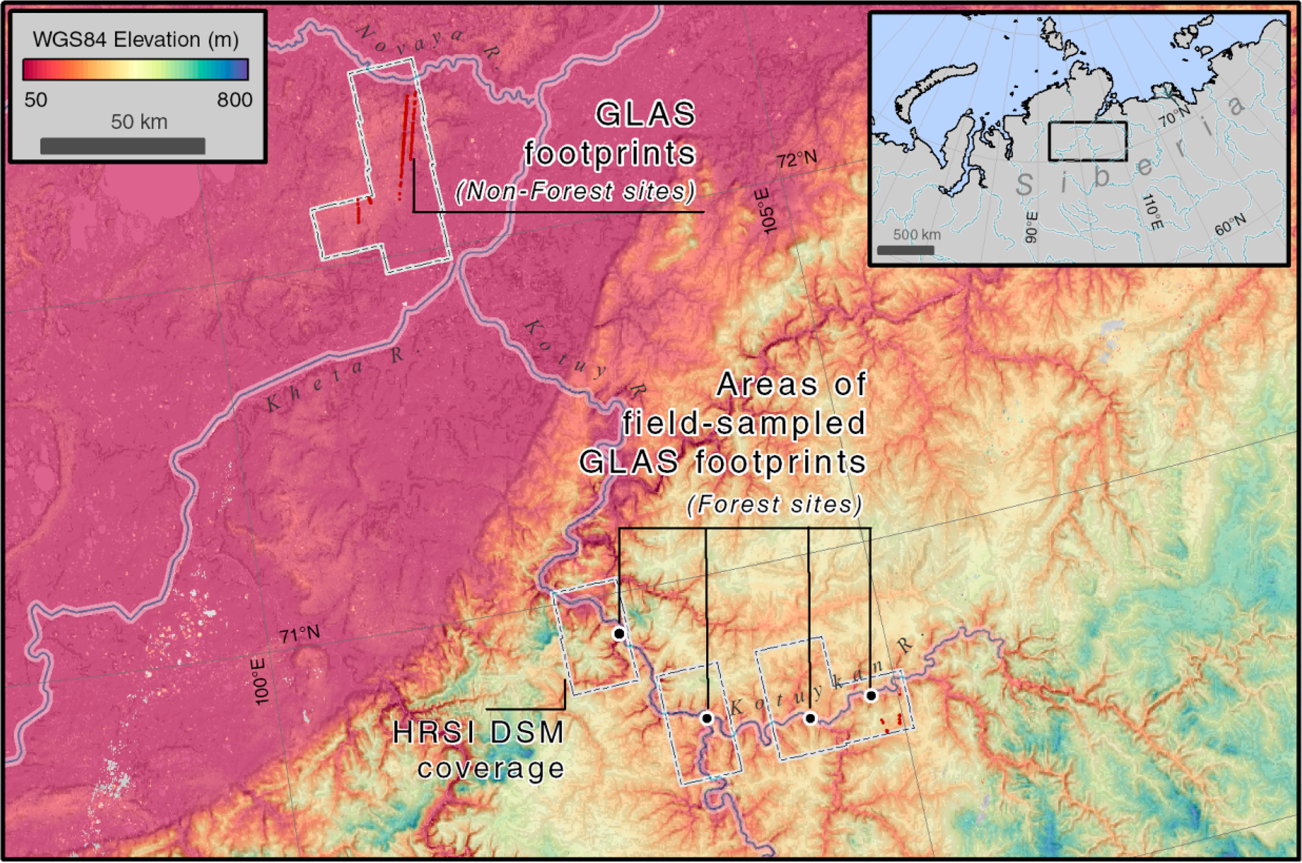
We analyzed ground measurements of individual tree heights, GLAS- and HRSIWV1 DSM - derived measurements of ground surface elevation, and spaceborne estimates (i.e., a combination of GLAS and HRSIWV1 DSM measurements) of maximum forest canopy heights in sparse Larix forests in northern Siberia (Figure 1). The ground-derived heights were collected in field surveys described in Section 2.1. The acquisition and processing of HRSIWV1 and GLAS data are described in Sections 2.2 and 2.3, respectively. The GLAS- and HRSIWV1-derived measurements of ground surface elevation were examined for non-forest and forest sites across northern Siberia. Finally, spaceborne forest canopy height estimates were calculated as the difference of ground surface elevations measurements (from either GLAS or HRSIWV1 DSMs) and canopy surface elevation measurements (from HRSIW1 DSMs) at field plots centered on GLAS footprints in forest stands. This analysis is detailed in Section 2.4.
2.1. Field Data
We examined a set of field data collected in Larix forest stands, part of a multi-year field NASA-lead campaign to collect forest structure measurements in the Central Siberian Plateau in 2007, 2008, and 2012. The set of cloud-free image data (described in Section 2.3) corresponding to field plots limited the geographic scope of the canopy height analysis described in Section 2.4 to plots along the Kotuykan River in the Anabar Plateau in northern Siberia, sampled in July–August 2008. Trees surveyed were located in primarily mature forest stands that exhibited no visible signs of recent disturbance from fire. Field plots were circular with a radius of 10 m or 15 m. The field plots were geo-located with hand-held global positioning system units to within ±5 m and centered on the elliptical GLAS footprints (50–60 m major axis) along elevational transects with little within-footprint slope (∼<10°). Plot boundaries were established from this center point using tape measurement of the plot’s radius to mark the plot’s edges along its circumference. The footprints selected for field sampling were those for which (1) footprint-centered field plots were representative of larger footprint sampled by GLAS and (2) the vegetation signal was not influenced by clouds or slope [26,38]. This field sampling protocol, used in a number of other studies, was designed for comparison with GLAS measurements of forest structure whereby each plot coincides with a unique GLAS footprint [26,38,62]. Thus, forest structure data was collected for a ground surface area that was most likely to coincide with the strongest portion of the transmitted GLAS LiDAR pulse. Additionally, ground plots were sized to provide sufficient sampling to characterize forest structure within a GLAS footprint while also allowing for sampling of a range of GLAS footprints across the study area.
Standard forestry techniques were used to collect tree diameters at breast height (1.3 m) and tree heights (clinometers for 97% of trees and tape measurement for 3%). The data used for this study included tree diameter at breast height (DBH) for all tree stems with DBH >3 cm (±0.1 cm) and corresponding tree heights for each tree in each plot. These plot data represented a range of sparse Larix forest conditions found across northern Siberia Larix forests, excluding prostrate Larix forms.
2.2. HRSI Data Acquisition and Processing
The HRSI data was acquired from the National Geospatial Intelligence Agency through an agreement with the US Government [50]. Cloud-free HRSI stereo pairs, i.e., two images of overlapping geographic extent acquired at different sensor view angles, were collected over northern Siberia in winter and summer 2012 by the Worldview-1 satellite. Each HRSIW1 stereo pair was acquired along track using the near simultaneous fore and aft images. These panchromatic images have a spatial resolution of ∼0.5 m. Cloud-free image pairs for Larix forests reveal individual and groups of Larix trees, regardless of season. Each image pair has a portion of geographic overlap used to derive surface elevations with the suite of stereo photogrammetric routines available from the open source NASA Ames Stereo Pipeline (ASP) 2.4 software available (along with the User’s Guide) at http://ti.arc.nasa.gov/tech/asr/intelligent-robotics/ngt/stereo/ [63].
The routines in ASP provide automatic stereo photogrammetric mapping of surface features. An image correlation sub-routine matches the corresponding pixels of image pairs, establishes epipolar geometry, and calculates the distance from the image focal plane to the earth surface features. A discussion of this process is presented in Ni et al., (2014) [64]. The advantage of the stereo pairs derived from along-track collection is that it provides images that are better suited for image matching algorithms. These image matching algorithms rely on radiometric and textural similarities among corresponding image pixel blocks. During the image matching portion of the routine, the linear camera model and the affine adaptive window mode option (subpixel mode = 2 in ASP) was used to provide the most accurate surface elevation results (Ames Stereo Pipeline User’s Guide, 2014). The horizontal accuracy of HRSIWV1 DSMs are expected to be <3.5 m [65], without the use of ground control. The use of ground control was not implemented in order to produce results from stereo pair processing that was fully automated.
For each stereo pair, a gridded HRSIWV1 DSM was generated at ∼0.4–0.7 m spatial resolution. This output HRSIWV1 DSM spatial resolution range was dictated by the native resolution of each stereo pair image, itself a function of sensor viewing geometry, which varied from image to image. The units of the pixel values were in meters above the WGS84 ellipsoid and represent the elevation of visible surface features. For forested areas, these DSMs provide a canopy surface elevation.
2.3. GLAS Data Acquisition and Processing
The GLAS level-2 global land surface laser altimetry was acquired from the National Snow and Ice Data Center ( http://nsidc.org/data/gla14). GLAS metrics (GLA14) were acquired for GLAS footprints from campaigns L3a, L3c, L3d, L3f, and L3g (October–November 2004, May–June and October–November in 2005 and 2006) across a broad extent of northern Siberia (60N–75N, 90E–110E). The 50–60 m GLAS footprints used were collected with a 1064 nm laser and have a horizontal geo-location accuracy of ∼4.5 m [54,66]. This dataset included those GLAS footprints sampled during field surveys. The cloud-free image extents for available HRSIW1 DSMs corresponded to non-forested and field-sampled forested GLAS footprints along the Kotuykan River and non-forested GLAS footprints north of the Kheta River.
The GLA14 data provided the ground surface elevation used in the analysis. Two GLA14 metrics were used to provide estimates of ground surface elevation. These metrics were (1) the elevation above the WGS84 ellipsoid of the GLAS waveform centroid (elev1) and (2) the GLAS waveform centroid height above the waveform’s lowest gaussian peak (centroid), which was assumed to represent the average ground surface elevation within a footprint. The original GLA14 elevation values in the TOPEX/Poseidon ellipsoid were converted to WGS84 ellipsoid values to account for the 71 cm vertical shift in our study area. These GLA14 metrics were used to derive a single ground surface elevation at field plot centers in two ways. The first was to subtract the height of the centroid from the elevation of the centroid (elev2). The second was to simply use the elevation of the centroid (elev1). Finally, the length of the waveform from signal beginning to signal end (wflen) was used for filtering out data whose waveforms may have been elongated due to terrain slope or cloud contamination. These metrics have been used previously as part of algorithms to derive canopy heights for GLAS footprints [23,33].
2.4. Analysis
A two-step process was used to examine the uncertainty of forest canopy height estimates using a combination of GLAS ground elevation and HRSIW1 DSM-derived surface elevation. First, we examined the correlation and uncertainty (the bootstrapped root mean square difference; RMSD) between flat ground surface elevation measurements from coincident locations measured by both GLAS and HRSIWV1 DSMs at unforested (i.e., tundra) and forested sites in northern Siberia. This was done to quantify the relative difference between ground surface elevation measurements from each sensor for land covers in which (1) the ground surface elevation measurements are not obscured by trees (Non-Forest); and (2) the ground surface is partially obscured by trees (Forest). The Non-Forest sites were 10 m radius circles centered on GLAS footprints that were classified as free of tree or high shrub vegetation. This classification was done in a geographic information system by overlaying GLAS footprints on HRSIW1, manually interpreting the HRSIWV1 for shrub and tree cover, and then manually selecting only those GLAS footprints that were free of such vegetation. The Forest sites were 10 m radius circles centered on those GLAS footprints for which in-situ field data was collected in forest plots. The ground surface elevation from HRSIW1 DSMs was calculated as the minimum value of all DSM pixels within a plot (dsmmin).
Second, we examined the relationship of spatially coincident measurements of maximum canopy height from field plots to those derived from spaceborne estimates (a combination of HRSIWV1 DSM and GLAS data). To do this we (1) computed spaceborne estimates of maximum canopy height at the plot scale and paired them with the height of the tallest tree (maximum tree height) of the coincident field plot; (2) filtered this set of paired field and spaceborne data to exclude those spaceborne estimates that did not meet thresholds for spaceborne data quality for short stature forest stands; and (3) computed a linear model of the relationship and performed statistical bootstrapping of the R2 and root mean square error (RMSE).
To compute spaceborne estimates of maximum canopy height at the plot scale, spatially coincident DSM pixel values and GLAS metrics were examined for each field plot. Field plots were represented by 10 m radius circles, centered on GLAS footprints, which corresponded to the size of the majority of plots established in the field. Based on the size of each circle and the spatial resolution of the DSMs, there were ∼2000 DSM pixels that were entirely within the boundary of a corresponding GLAS footprint-centered, 10 m radius circle representing the field plot. Summary statistics were compiled from the set of pixels corresponding to each circle to provide an estimate of maximum canopy surface elevation (dsmmax: the maximum value of the plot’s pixels) as well as potential ground surface elevation (dsmmin: the minimum value of the plot’s pixels). The final ground elevation (elevground) was determined from the minimum of the GLAS metrics elev1, elev2, along with the DSM-derived dsmmin. Spaceborne maximum canopy height for each plot was then calculated by subtracting elevground from dsmmax. These spaceborne estimates were linked to the corresponding maximum tree height values of all trees of a given field plot.
The set of field plots used were filtered according to two conditions. The final set of field plots were those for which; (1) the coincident HRSIWV1 data had stereo pair convergence angles >35 degrees; and (2) the coincident GLAS waveform offset distance from signal beginning to end (wflen) <16 m [67]. These conditions were used to reduce the effect of feature height errors associated with low convergence angles [59–61], slope and cloud contamination on the comparison of field- and spaceborne-derived heights. The remaining plots featured a set of trees 97% of which were less than 10 m in height.
Linear regression was used to model the relationship of the field plot and spaceborne maximum canopy height measurements. With this model, field-derived canopy height was the dependent variable to conform to the approach of using spaceborne measurements to predict those that are ground-based. The fit and uncertainty of this model was quantified using model bootstrapping. This produced a distribution for the model’s R2 and root moon square error (RMSE) by repeated sampling (with replacement) of the data.
3. Results
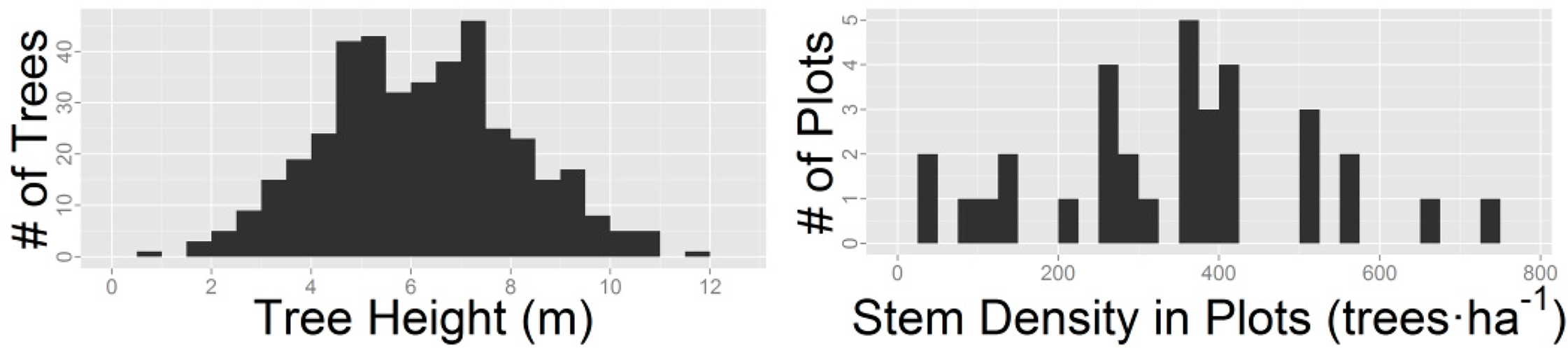
The histogram in Figure 2 shows stem density for trees in the 33 forested field plots that remained available for analysis after data filtering. It explains the range of trees (>3 cm DBH) per hectare for these forested plots centered on GLAS footprints that remained after HRSIWV1 DSM convergence angle and GLAS wflen thresholds were applied. At these 33 plots, 410 trees (Larix sp.) were surveyed for DBH and height. The heights of 400 trees were measured with clinometers and those of the remaining 10 directly with standard tape measurements.
The relative difference between GLAS and HRSIW1 DSM ground elevation measurements was examined using 355 GLAS footprints in Non-Forest (tundra) sites and 73 in Forest sites in northern Siberia (Figure 3). The model comparing the two ground elevation measurements in both Non-Forest and Forest shows a close 1-to-1 fit across the ∼350 and ∼300 m elevation ranges (slope = 1, p < 0.001). The DSM and GLAS measurements have a difference in bias between Non-Forest (y-intercept = −1.3 m, p < 0.001) and Forest locations (y-intercept = −4.1 m, p < 0.01) of 2.8 m. The bootstrapped root mean square difference (RMSD) of ground elevations from the Non-Forest model had a 95% confidence interval (CI) of ±0.90 m–1.06 m while that of the Forest model was ±2.26 m–3.40 m. These GLAS ground elevation results for Non-Forest are similar to those of recent studies that examined ground elevation retrieval from GLAS [57,67].
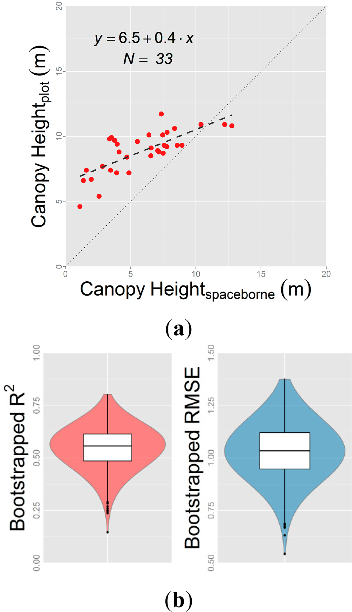
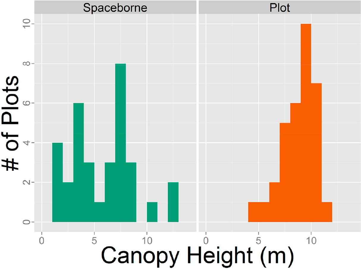
The linear model for predicting plot maximum canopy height is reported in Figure 4a (model coefficients’ p < 0.001). Figure 4b depicts the bootstrapped R2 and RMSE distributions of the model in 4a. This model corrects for the spaceborne measurements underestimating heights less than 10 m, particularly heights <5 m. The bootstrapped RMSE ranged from 0.86 m to 1.37 m at the 95% confidence level. This error was based on a mean bootstrapped R2 of 0.55, which ranged from 0.36 to 0.74 at the 95% confidence level. The histograms in Figure 5 show the distributions of maximum heights from both the field and the spaceborne measurements. Maximum plot heights measured in the field range from ∼5 m to ∼12 m. Those derived from spaceborne measurements ranged from ∼1 m to ∼12 m.
4. Discussion
4.1. Spaceborne Canopy Height and Its Sources of Uncertainty
This analysis coupled a comparison of measurements of ground surface elevations from two satellites with a comparison of field- and spaceborne-derived canopy height estimates. The analysis of ground surface elevation shows that GLAS data provides consistently lower elevation measurements than those of coincident HRSIWV1 DSMs for Non-Forest, and in particular Forest, sites. This supports the technique of combining coincident GLAS ground surface elevations with HRSIWV1 DSM canopy surface elevations to derive spaceborne estimates of canopy height. The DSMs provide an estimate of canopy surface elevation in this study, where GLAS is mostly insensitive to the subtle structural signals of sparse forest cover. The DSMs are less reliable for providing the lowest ground surface elevation, so for this measurement, the ground surface elevation is best determined as the minimum value of both GLAS and DSM elevations. This combined use of spaceborne data was used to compute spaceborne canopy height estimates in sparse forest cover. The canopy height analysis indicates that GLAS and HRSIW1 DSMs predict field plot estimates of maximum canopy height in the sparsely forested stands of the taiga-tundra ecotone with an uncertainty range of ±0.86–1.37 m at the plot-scale (∼314–707 m2). However, these estimates are based on only a moderate model fit.
The canopy height model is noisy and the relationship suggests a bias from spaceborne maximum canopy heights. This bias arises from the apparent tendency of this combination of satellite data to underestimate plot-derived maximum plot heights <10 m. This underestimation could be due to either or both of the following, (1) an overestimation of ground surface elevation or (2) an underestimation of canopy surface elevation. We believe it is the latter for two reasons. The first reason is that the use of GLAS ground elevation provides a lower elevation relative to the DSM (Figure 3), decreasing the likelihood of ground elevation overestimation, particularly in sparse forests. Second, this underestimation of maximum height is similar to the bias seen in both waveform and small footprint LiDAR, and may occur because the tops of trees are either not resolved or detected, and the remote measurement is likely coming from lower in the canopy [68,69]. For sparse Larix forest stands, the difficulty in resolving the top of trees is not surprising, given the relatively small canopy area of the mature growth forms found in northern Siberia. Thus, model uncertainty may also be related to maximum tree heights in plots not sufficiently representing that which the spaceborne data reflects. Finally, while efforts were made to align field plots with HRSIWV1 DSM data, compounded horizontal geo-location errors among field plots and DSM pixels can influence model fit and uncertainty. Thus, the magnitude of error from plot-scale spaceborne canopy height is particularly sensitive to data at finer scales [70]. This increases the difficulty of reducing uncertainty at the plot-scale across broad regions, as trade-offs between the size of plots and the number of plots surveyed are usually made during expensive and time consuming field expeditions. Gaps between field and HRSIWV1 data (∼4 years) are not expected to be significant sources of error given the age and relatively slow growth of trees in this area [71–73].
The lower RMSD between ground elevation from GLAS and HRSIWV1 DSMs at Non-Forest sites relative to Forest sites suggests the contribution of GLAS ground elevation to canopy height estimates is an improvement on those from stereo photogrammetry alone. However, an analysis solely focused on this difference was not performed. Stereo photogrammetric estimates of ground elevation estimates within forested areas are highly uncertain [74,75]. The use of GLAS as a means of achieving reliable ground surface elevation measurements, particularly in sparse forests, is a novel technique which can potentially decrease the uncertainty of millions of TTE vegetation height estimates at the plot-scale when complemented with HRSI DSMs, without the use of airborne data. The trade-off, however, is that canopy height from this method is available as samples coincident with GLAS footprints rather than as a continuous map variable across the extent of the HRSI field of view.
The model can be applied to all GLAS footprints with coincident DSMs in Larix stands to estimate stand height. However, the model was built from 33 field plots and the limited sample size is in part responsible for the broad uncertainty of the model fit (the distribution of the bootstrapped R2 at the 95% confidence level). The inherent drawback for modeling Larix stand height is that uncertainty estimates are less robust with lower R2. The model error is similar to other reported canopy height model errors from high-resolution spaceborne imagery [76], although the model in this study was built from sparse and short stature Larix, primarily between 5 and 10 m in height. Most of the available field plot data collected in Siberian Larix stands were not used because coincident DSMs were not available at the time of the analysis. However, as more DSMs become available, the model can be updated to provide a more robust estimate of the stand height uncertainty from spaceborne remote sensing at the plot-scale.
4.2. Future Work
There is a unique need for high resolution spaceborne estimates of vegetation structure across the taiga-tundra ecotone, and in Siberia, in particular. This need is driven by the importance of TTE vegetation on regional and global climate, its propensity for change, the subtle yet relevant signal of its vegetation, and the difficulty of collecting field and airborne data. Existing global level estimates of vegetation height, suited for depicting average landscape-scale attributes, are likely to be too coarse and uncertain for monitoring site-specific and spatially variable changes in the sparse forests of the TTE that have been expected and documented [7,20,77,78].
This study’s technique provides an opportunity to examine detailed vegetation structure in sparse forests across broad extents in regions difficult to assess through field and airborne survey. Applying this model across thousands of forested GLAS footprints with coincident DSMs in northern Siberia is a potential next step for examining uncertainty in spaceborne-derived forest structure across a TTE landscape. These empirically derived sample heights can be averaged according to forest patches, attributing the two-dimensional patches with statistical estimates of vertical forest structure and its uncertainty. This scaling-up to forest patch-level estimates of canopy height and its uncertainty can then be empirically related to coarser remote sensing data (ASTER, Landsat, ALOS PALSAR) to extend patch-level estimates of canopy height and its uncertainty across regions. This potential for extending estimates across remote regions is enabled through the automated processing of DSMs (without the use of ground control points). While height estimates from DSMs can be improved with ground control, these data are typically not available in remote areas and not practical to apply when processing large volumes of data across broad extents.
The way in which satellite estimates of sparse and short stature forest canopy height may change with DSMs derived from other image pairs was not tested. Such an endeavor would involve analyzing repeated stereo pair DSM measurements at each plot. With this approach, a study could examine the effects of a number of variables on the uncertainty of canopy height estimates for a continuum of forest stand structural arrangements (sparse and short, sparse and tall, dense and short, dense and tall). These variables would include seasonality, satellite geometry, snow cover/depth, and slope/aspect. Furthermore, repeated DSM measurements add vegetation height information, building a distribution of height measurements at a given location. This will help refine spaceborne canopy height measurements, by reducing uncertainty and revealing the fundamental bias (assuming one in fact exists) associated with TTE canopy surface measurements from HRSI DSMs. The opportunity for high-resolution monitoring of the TTE is growing. The archives of existing GLAS along with increasing HRSI stereo coverage (used to derive DSMs) will continue to add complementary pieces of information on TTE vegetation structure, particularly forest height. The launch of NASA’s ICESat-2 satellite will add measurements of vegetation height and ground elevation to existing datasets, and will increase the spatial and temporal sampling of TTE vegetation structure. While significant uncertainties may exist from TTE vegetation structure estimates derived from ICESat-2 data alone, photon-counting LiDAR measurements in tandem with other datasets may help reduce measurement uncertainty of forest characteristics at critical scales.
5. Conclusions
At the plot-scale in northern Siberia Larix forests, complementary measurements from GLAS and HRSIWV1 DSMs can produce canopy height estimates in sparse TTE stands primarily <10 m in height. These TTE stand measurements combine archival ground elevation from GLAS and current canopy surface elevation from HRSI stereo image pairs. With a linear model, spaceborne canopy height predicted these TTE stand heights, between ∼5 m and ∼10 m tall, with an R2 of 0.55 (0.36–0.74, 95% CI) and an uncertainty ranging from ±0.86 to 1.37 m.
This study provides a means for directly measuring TTE forest height from a combination of LiDAR and multispectral spaceborne sensors. This uncertainty of these height estimates in TTE stands can be better characterized by analyzing GLAS and HRSI DSMs across a broader range of sensor and target conditions. The use of HRSI DSMs compiled from image pairs whose satellite geometry minimize the uncertainty in height estimates for TTE stands will clarify the potential for plot-scale measurements of subtle vegetation structure signals from spaceborne data. Scaling up these plot-scale height and uncertainty measurements to the forest patch scale will allow these estimates to be spatially continuous, rather than limited to GLAS footprint samples.
Acknowledgments
This work was supported by NASA’s Terrestrial Ecology Program and was made possible in part through field expedition contributions from Ross Nelson, Viacheslav Kharuk, Sergey Im, Pavel Oskorbin, and Muhktar Naurzbaev. We acknowledge the work of Oleg Alexandrov and Zachary Moratto for development and on-going support of NASA’s Ames Stereo Pipeline software. We thank the 5 anonymous reviewers for helping to significantly improve this manuscript.
Author Contributions
Paul Montesano partook in the field data collection, conceived and implemented the research design, performed a portion of the data acquisition, analyzed the datasets and wrote the manuscript. Guoqing Sun partook in the field data collection, performed a portion of the data acquisition and provided feedback on data analysis techniques. Ralph Dubayah provided feedback and advice regarding underlying research emphasis and direction. Jon Ranson partook in the field data collection, and provided manuscript feedback and project funding.
Conflicts of Interest
The authors declare no conflicts of interest.
References
- Bonan, G.B.; Pollard, D.; Thompson, S.L. Effects of boreal forest vegetation on global climate. Nature 1992, 359, 716–718. [Google Scholar]
- Chapin, F., III; Sturm, M.; Serreze, M.; McFadden, J.P.; Key, J.R.; Lloyd, A.H.; McGuire, A.D.; Rupp, T.S.; Lynch, A.H.; Schimel, J.P.; et al. Role of land-surface changes in arctic summer warming. Science 2005, 310, 657–660. [Google Scholar]
- Ranson, K.J.; Montesano, P.M.; Nelson, R. Object-based mapping of the circumpolar taiga—Tundra ecotone with MODIS tree cover. Remote Sens. Environ 2011, 115, 3670–3680. [Google Scholar]
- Harsch, M.; Hulme, P.; McGlone, M.; Duncan, R. Are treelines advancing? A global meta-analysis of treeline response to climate warming. Ecol. Lett 2009, 12, 1040–1049. [Google Scholar]
- Elmendorf, S.C.; Henry, G.H.R.; Hollister, R.D.; Björk, R.G.; Boulanger-Lapointe, N.; Cooper, E.J.; Cornelissen, J.H.C.; Day, T.A.; Dorrepaal, E.; Elumeeva, T.G.; et al. Plot-scale evidence of tundra vegetation change and links to recent summer warming. Nat. Clim. Change 2012, 2, 453–457. [Google Scholar]
- Epstein, H.E.; Myers-Smith, I.; Walker, D.A. Recent dynamics of arctic and sub-arctic vegetation. Environ. Res. Lett 2013. [Google Scholar] [CrossRef]
- Kharuk, V.I.; Ranson, K.J.; Im, S.T.; Naurzbaev, M.M. Forest-tundra larch forests and climatic trends. Russ. J. Ecol 2006, 37, 291–298. [Google Scholar]
- Loranty, M.M.; Goetz, S.J. Shrub expansion and climate feedbacks in Arctic tundra. Environ. Res. Lett 2012. [Google Scholar] [CrossRef]
- Bonfils, C.J.W.; Phillips, T.J.; Lawrence, D.M.; Cameron-Smith, P.; Riley, W.J.; Subin, Z.M. On the influence of shrub height and expansion on northern high latitude climate. Environ. Res. Lett 2012. [Google Scholar] [CrossRef]
- Blok, D.; Heijmans, M.; Schaepman-Strub, G.; Kononov, A.V.; Maximov, T.C.; Berendse, F. Shrub expansion may reduce summer permafrost thaw in Siberian tundra. Glob. Change Biol 2010, 16, 1296–1305. [Google Scholar]
- Myers-Smith, I.H.; Forbes, B.C.; Wilmking, M.; Hallinger, M.; Lantz, T.; Blok, D.; Tape, K.D.; Macias-Fauria, M.; Sass-Klaassen, U.; Lévesque, E.; et al. Shrub expansion in tundra ecosystems: Dynamics, impacts and research priorities. Environ. Res. Lett 2011. [Google Scholar] [CrossRef]
- Lawrence, D.M.; Swenson, S.C. Permafrost response to increasing Arctic shrub abundance depends on the relative influence of shrubs on local soil cooling versus large-scale climate warming. Environ. Res. Lett 2011. [Google Scholar] [CrossRef]
- Pearson, R.G.; Phillips, S.J.; Loranty, M.M.; Beck, P.S.A.; Damoulas, T.; Knight, S.J.; Goetz, S.J. Shifts in Arctic vegetation and associated feedbacks under climate change. Nat. Clim. Change 2013, 3, 1–5. [Google Scholar]
- Loranty, M.M.; Berner, L.T.; Goetz, S.J.; Jin, Y.; Randerson, J.T. Vegetation controls on northern high latitude snow-albedo feedback: Observations and CMIP5 model predictions. Glob. Change Biol 2013, 20, 594–606. [Google Scholar]
- MacDonald, G.M.; Kremenetski, K.V.; Beilman, D.W. Climate change and the northern Russian treeline zone. Philos. Trans. R. Soc. B 2008, 363, 2283–2299. [Google Scholar]
- Epstein, H.E.; Beringer, J.; Gould, W.A.; Lloyd, A.H.; Thompson, C.D.; Chapin, F.S.; Michaelson, G.J.; Ping, C.L.; Rupp, T.S.; Walker, D.A. The nature of spatial transitions in the Arctic. J. Biogeogr 2004, 31, 1917–1933. [Google Scholar]
- Ropars, P.; Boudreau, S. Shrub expansion at the forest—Tundra ecotone: Spatial heterogeneity linked to local topography. Environ. Res. Lett 2012. [Google Scholar] [CrossRef]
- Lloyd, A.H.; Bunn, A.G.; Berner, L.T. A latitudinal gradient in tree growth response to climate warming in the Siberian taiga. Glob. Change Biol 2011, 17, 1935–1945. [Google Scholar]
- Loranty, M.M.; Goetz, S.J.; Beck, P.S.A. Tundra vegetation effects on pan-Arctic albedo. Environ. Res. Lett 2011. [Google Scholar] [CrossRef]
- Hofgaard, A.; Harper, K.A.; Golubeva, E. The role of the circumarctic forest—Tundra ecotone for Arctic biodiversity. Biodiversity 2012, 13, 174–181. [Google Scholar]
- Hansen, M.C.; Potapov, P.V.; Moore, R.; Hancher, M.; Turubanova, S.A.; Tyukavina, A.; Thau, D.; Stehman, S.V.; Goetz, S.J.; Loveland, T.R.; et al. High-resolution global maps of 21st-century forest cover change. Science 2013, 342, 850–853. [Google Scholar]
- Lefsky, M.A. A global forest canopy height map from the Moderate Resolution Imaging Spectroradiometer and the Geoscience Laser Altimeter System. Geophys. Res. Lett 2010. [Google Scholar] [CrossRef]
- Lefsky, M.A.; Harding, D.J.; Keller, M.; Cohen, W.B.; Carabajal, C.C.; Espirito-Santo, F.D.B.; Hunter, M.O.; de Oliveira, R., Jr. Estimates of forest canopy height and aboveground biomass using ICESat. Geophys. Res. Lett 2005. [Google Scholar] [CrossRef]
- Simard, M.; Pinto, N.; Fisher, J.B.; Baccini, A. Mapping forest canopy height globally with spaceborne lidar. J. Geophys. Res.: Biogeosci 2011. [Google Scholar] [CrossRef]
- Los, S.O.; Rosette, J.A.B.; Kljun, N.; North, P.R.J.; Chasmer, L.; Suárez, J.C.; Hopkinson, C.; Hill, R.A.; van Gorsel, E.; Mahoney, C.; et al. Vegetation height and cover fraction between 60°S and 60°N from ICESat GLAS data. Geosci. Model Dev 2012, 5, 413–432. [Google Scholar]
- Neigh, C.S.R.; Nelson, R.F.; Ranson, K.J.; Margolis, H.A.; Montesano, P.M.; Sun, G.; Kharuk, V.; Næsset, E.; Wulder, M.A.; Andersen, H.-E. Taking stock of circumboreal forest carbon with ground measurements, airborne and spaceborne LiDAR. Remote Sens. Environ 2013, 137, 274–287. [Google Scholar]
- Santoro, M.; Cartus, O.; Fransson, J.; Shvidenko, A.; McCallum, I.; Hall, R.; Beaudoin, A.; Beer, C.; Schmullius, C. Estimates of forest growing stock volume for Sweden, Central Siberia, and Québec using Envisat Advanced Synthetic Aperture Radar backscatter data. Remote Sens 2013, 5, 4503–4532. [Google Scholar]
- Baccini, A.; Laporte, N.; Goetz, S. A first map of tropical Africa’s above-ground biomass derived from satellite imagery. Environ. Res. Lett 2008. [Google Scholar] [CrossRef]
- Cartus, O.; Kellndorfer, J.; Rombach, M.; Walker, W. Mapping canopy height and growing stock volume using airborne lidar, ALOS PALSAR and Landsat ETM. Remote Sens 2012, 4, 3320–3345. [Google Scholar]
- Duncanson, L.I.; Niemann, K.O.; Wulder, M.A. Estimating forest canopy height and terrain relief from GLAS waveform metrics. Remote Sens. Environ 2010, 114, 138–154. [Google Scholar]
- Ranson, K.; Sun, G.; Kharuk, V.; Kovacs, K. Assessing tundra—Taiga boundary with multi-sensor satellite data. Remote Sens. Environ 2004, 93, 283–295. [Google Scholar]
- Ranson, K.; Sun, G. An evaluation of AIRSAR and SIR-C/X-SAR images for mapping northern forest attributes in Maine, USA. Remote Sens. Environ 1997, 59, 203–222. [Google Scholar]
- Sun, G.; Ranson, K.J.; Masek, J.; Guo, Z.; Pang, Y.; Fu, A.; Wang, D. Estimation of tree height and forest biomass from GLAS data. J. For. Plan 2008, 13, 157–164. [Google Scholar]
- Heiskanen, J. Tree cover and height estimation in the Fennoscandian tundra—Taiga transition zone using multiangular MISR data. Remote Sens. Environ 2006, 103, 97–114. [Google Scholar]
- Wulder, M.A.; Seemann, D. Forest inventory height update through the integration of lidar data with segmented Landsat imagery. Can. J. Remote Sens 2003, 29, 536–543. [Google Scholar]
- Wulder, M.; Han, T.; White, J.; Sweda, T.; Tsuzuki, H. Integrating profiling LIDAR with Landsat data for regional boreal forest canopy attribute estimation and change characterization. Remote Sens. Environ 2007, 110, 123–137. [Google Scholar]
- Nelson, R.; Ståhl, G.; Holm, S.; Gregoire, T.; Næsset, E.; Gobakken, T. Using airborne & space lidars for large-area inventory. Proceedings of the 2010 IEEE International Geoscience and Remote Sensing Symposium (IGARSS), Honolulu, HI, USA, 25–30 July 2010; pp. 2463–2466.
- Montesano, P.M.; Nelson, R.F.; Dubayah, R.O.; Sun, G.; Cook, B.D.; Ranson, K.J.R.; Næsset, E.; Kharuk, V. The uncertainty of biomass estimates from LiDAR and SAR across a boreal forest structure gradient. Remote Sens. Environ 2014. in press.. [Google Scholar]
- Hensley, S.; Oveisgharan, S.; Saatchi, S.; Simard, M.; Ahmed, R.; Haddad, Z. An error model for biomass estimates derived from polarimetric radar backscatter. IEEE Trans Geosci. Remote Sens 2014, 52, 4065–4082. [Google Scholar]
- Nelson, R. Model effects on GLAS-based regional estimates of forest biomass and carbon. Int. J. Remote Sens 2010, 31, 1359–1372. [Google Scholar]
- Esper, J.; Schweingruber, F.H. Large-scale treeline changes recorded in Siberia. Geophys. Res. Lett 2004. [Google Scholar] [CrossRef]
- Montesano, P.; Nelson, R.; Sun, G.; Margolis, H.; Kerber, A.; Ranson, K. MODIS tree cover validation for the circumpolar taiga-tundra transition zone. Remote Sens. Environ 2009, 113, 2130–2141. [Google Scholar]
- Berner, L.T.; Beck, P.S.A.; Loranty, M.M.; Alexander, H.D.; Mack, M.C.; Goetz, S.J. Cajander larch (Larix cajanderi) biomass distribution, fire regime and post-fire recovery in northeastern Siberia. Biogeosciences 2012, 9, 3943–3959. [Google Scholar]
- Urban, M.; Forkel, M.; Eberle, J.; Hüttich, C.; Schmullius, C.; Herold, M. Pan-arctic climate and land cover trends derived from multi-variate and multi-scale analyses (1981–2012). Remote Sens 2014, 6, 2296–2316. [Google Scholar]
- Neigh, C.; Masek, J.; Bourget, P.; Cook, B.; Huang, C.; Rishmawi, K.; Zhao, F. Deciphering the precision of stereo IKONOS canopy height models for US forests with G-LiHT airborne lidar. Remote Sens 2014, 6, 1762–1782. [Google Scholar]
- Petrou, Z.I.; Manakos, I.; Stathaki, T.; Tarantino, C.; Adamo, M.; Blonda, P. A vegetation height classification approach based on texture analysis of a single VHR image. IOP Conf. Ser. Earth Environ. Sci 2014. [Google Scholar] [CrossRef]
- Hobi, M.L.; Ginzler, C. Accuracy assessment of digital surface models based on WorldView-2 and ADS80 stereo remote sensing data. Sensors 2012, 12, 6347–6368. [Google Scholar]
- Praks, J.; Hallikainen, M.; Antropov, O.; Molina, D. Boreal forest tree height estimation from interferometric TanDEM-X images. Proceedings of the 2012 IEEE International Geoscience and Remote Sensing Symposium (IGARSS), Munich, Germany, 20–27 July 2012; pp. 1262–1265.
- Hirschmugl, M.; Ofner, M.; Raggam, J.; Schardt, M. Single tree detection in very high resolution remote sensing data. Remote Sens. Environ 2007, 110, 533–544. [Google Scholar]
- Neigh, C.S.; Masek, J.G.; Nickeson, J.E. High-resolution satellite data open for government research. Eos Trans. Am. Geophys. Union 2013, 94, 121–123. [Google Scholar]
- Boyle, S.A.; Kennedy, C.M.; Torres, J.; Colman, K.; Pérez-Estigarribia, P.E.; de la Sancha, N.U. High-resolution satellite imagery is an important yet underutilized resource in conservation biology. PLoS One 2014. [Google Scholar] [CrossRef]
- Zwally, H.J.; Schutz, B.; Abdalati, W.; Abshire, J.; Bentley, C.; Brenner, A.; Bufton, J.; Dezio, J.; Hancock, D.; Harding, D. ICESat’s laser measurements of polar ice, atmosphere, ocean, and land. J. Geodyn 2002, 34, 405–445. [Google Scholar]
- Chopping, M. CANAPI: Canopy analysis with panchromatic imagery. Remote Sens. Lett 2011, 2, 21–29. [Google Scholar]
- Urban, T.J.; Shutz, B.E.; Neuenschwander, A.L. A survey of ICESat coastal altimetry applications: Continental coast, open ocean island, and inland river. Terr. Atmos. Ocean. Sci 2008, 19, 1–19. [Google Scholar]
- Carabajal, C.C.; Harding, D.J. SRTM C-band and ICESat laser altimetry elevation comparisons as a function of tree cover and relief. Photogramm. Eng. Remote Sens 2006, 72, 287–298. [Google Scholar]
- Yi, D.; Zwally, H.J.; Sun, X. ICESat measurement of Greenland ice sheet surface slope and roughness. Ann. Glaciol 2005, 42, 83–89. [Google Scholar]
- Popescu, S.C.; Zhao, K.; Neuenschwander, A.; Lin, C. Satellite lidar vs. small footprint airborne lidar: Comparing the accuracy of aboveground biomass estimates and forest structure metrics at footprint level. Remote Sens. Environ 2011, 115, 2786–2797. [Google Scholar]
- Jacobsen, K. DEM Generation from Satellite Data. Available online: http://www.earsel.org/tutorials/Jac_03DEMGhent_red.pdf (accessed on 11 October 2014).
- Li, R.; Zhou, F.; Niu, X.; Di, A.K. Integration of Ikonos and QuickBird imagery for geopositioning accuracy analysis. Photogramm. Eng. Remote Sens 2007, 73, 1067–1074. [Google Scholar]
- Li, R.; Niu, X.; Liu, C.; Wu, B.; Deshpande, S. Impact of imaging geometry on 3D geopositioning accuracy of stereo IKONOS imagery. Photogramm. Eng. Remote Sens 2009, 75, 1119–1125. [Google Scholar]
- Aguilar, M.A.; del Mar Saldana, M.; Aguilar, F.J. Generation and quality assessment of stereo-extracted DSM from GeoEye-1 and WorldView-2 imagery. IEEE Trans. Geosci. Remote Sens 2014, 52, 1259–1271. [Google Scholar]
- Nelson, R.; Ranson, K.J.; Sun, G.; Kimes, D.S.; Kharuk, V.; Montesano, P. Estimating Siberian timber volume using MODIS and ICESat/GLAS. Remote Sens. Environ 2009, 113, 691–701. [Google Scholar]
- Moratto, Z.M.; Broxton, M.J.; Beyer, R.A.; Lundy, M.; Husmann, K. Ames stereo pipeline, NASA ’s open source automated stereogrammetry software. Proceedings of the 41st Lunar and Planetary Science Conference, Woodlands, TX, USA, 1–5 March 2010; p. 2364.
- Ni, W.; Ranson, K.J.; Zhang, Z.; Sun, G. Features of point clouds synthesized from multi-view ALOS/PRISM data and comparisons with LiDAR data in forested areas. Remote Sens. Environ 2014, 149, 47–57. [Google Scholar]
- Capaldo, P.; Crespi, M.; Fratarcangeli, F.; Nascetti, A.; Pieralice, F. DSM generation from high resolution imagery: Applications with WorldView-1 and Geoeye-1. Ital. J. Remote Sens 2012, 44, 42–53. [Google Scholar]
- Duong, H; Lindenbergh, R.; Pfeifer, N.; Vosselman, G. ICESat full waveform altimetry compared to airborne laser scanning altimetry over The Netherlands. IEEE Trans. Geosci. Remote Sens 2009, 47, 3365–3378. [Google Scholar]
- Sun, G.; Ranson, K.; Kimes, D.; Blair, J.; Kovacs, K. Forest vertical structure from GLAS: An evaluation using LVIS and SRTM data. Remote Sens. Environ 2008, 112, 107–117. [Google Scholar]
- Peterson, B.; Nelson, K.; Wylie, B. Towards integration of GLAS into a national fuel mapping program. Photogramm. Eng. Remote Sens 2013, 79, 175–183. [Google Scholar]
- Wasser, L.; Day, R.; Chasmer, L.; Taylor, A. Influence of vegetation structure on lidar-derived canopy height and fractional cover in forested riparian buffers during leaf-off and leaf-on conditions. PLoS One 2013. [Google Scholar] [CrossRef]
- Frazer, G.W.; Magnussen, S.; Wulder, M.A.; Niemann, K.O. Simulated impact of sample plot size and co-registration error on the accuracy and uncertainty of LiDAR-derived estimates of forest stand biomass. Remote Sens. Environ 2011, 115, 636–649. [Google Scholar]
- Kajimoto, T.; Osawa, A.; Usoltsev, V.A.; Abaimov, A.P. Biomass and productivity of siberian larch forest ecosystems. In Ecological Studies Ecological Studies; Springer: Dordrecht, The Netherlands, 2010; Volume 209, pp. 99–122. [Google Scholar]
- Osawa, A.; Kajimoto, T. Development of stand structure in larch forests. In Ecological Studies Ecological Studies; Springer: Dordrecht, The Netherlands, 2010; Volume 209, pp. 123–148. [Google Scholar]
- Kharuk, V.I.; Ranson, K.J.; Im, S.T.; Oskorbin, P.A.; Dvinskaya, M.L.; Ovchinnikov, D.V. Tree-line structure and dynamics at the northern limit of the larch forest: Anabar Plateau, Siberia, Russia. Arct. Antarct. Alp. Res 2013, 45, 526–537. [Google Scholar]
- Vepakomma, U.; St-Onge, B.; Kneeshaw, D. Response of a boreal forest to canopy opening: Assessing vertical and lateral tree growth with multi-temporal lidar data. Ecol. Appl 2011, 21, 99–121. [Google Scholar]
- Raggam, H.; Franke, M.; Ofner, M.; Gutjahr, K. Accuracy assessment of vegetation height mapping using spaceborne IKONOS as well as aerial UltraCam stereo images. Proceedings of the EARSel 3D Remote Sensing Workshop, Porto, Portugal, 6–11 June 2005; pp. 1–12.
- Huang, H.; Cao, B. Experiment on extracting forest canopy height from Worldview-2. Proceedings of the 2011 Eighth International Conference on Fuzzy Systems and Knowledge Discovery (FSKD), Shanghai, China, 26–28 July; 2011; pp. 2614–2617. [Google Scholar]
- Holtmeier, F.K.; Broll, G. Sensitivity and response of northern hemisphere altitudinal and polar treelines to environmental change at landscape and local scales. Glob. Ecol. Biogeogr 2005, 14, 395–410. [Google Scholar]
- Naurzbaev, M.M.; Hughes, M.K.; Vaganov, E.A. Tree-ring growth curves as sources of climatic information. Quat. Res 2004, 62, 126–133. [Google Scholar]


© 2014 by the authors; licensee MDPI, Basel, Switzerland This article is an open access article distributed under the terms and conditions of the Creative Commons Attribution license (http://creativecommons.org/licenses/by/4.0/).
Share and Cite
Montesano, P.M.; Sun, G.; Dubayah, R.; Ranson, K.J. The Uncertainty of Plot-Scale Forest Height Estimates from Complementary Spaceborne Observations in the Taiga-Tundra Ecotone. Remote Sens. 2014, 6, 10070-10088. https://doi.org/10.3390/rs61010070
Montesano PM, Sun G, Dubayah R, Ranson KJ. The Uncertainty of Plot-Scale Forest Height Estimates from Complementary Spaceborne Observations in the Taiga-Tundra Ecotone. Remote Sensing. 2014; 6(10):10070-10088. https://doi.org/10.3390/rs61010070
Chicago/Turabian StyleMontesano, Paul M., Guoqing Sun, Ralph Dubayah, and Kenneth J. Ranson. 2014. "The Uncertainty of Plot-Scale Forest Height Estimates from Complementary Spaceborne Observations in the Taiga-Tundra Ecotone" Remote Sensing 6, no. 10: 10070-10088. https://doi.org/10.3390/rs61010070