Spatio-Temporal Analysis of Gyres in Oriented Lakes on the Arctic Coastal Plain of Northern Alaska Based on Remotely Sensed Images


Abstract
: The formation of oriented thermokarst lakes on the Arctic Coastal Plain of northern Alaska has been the subject of debate for more than half a century. The striking elongation of the lakes perpendicular to the prevailing wind direction has led to the development of a preferred wind-generated gyre hypothesis, while other hypotheses include a combination of sun angle, topographic aspect, and/or antecedent conditions. A spatio-temporal analysis of oriented thermokarst lake gyres with recent (Landsat 8) and historical (Landsat 4, 5, 7 and ASTER) satellite imagery of the Arctic Coastal Plain of northern Alaska indicates that wind-generated gyres are both frequent and regionally extensive. Gyres are most common in lakes located near the Arctic coast after several days of sustained winds from a single direction, typically the northeast, and decrease in number landward with decreasing wind energy. This analysis indicates that the conditions necessary for the Carson and Hussey (1962) wind-generated gyre for oriented thermokarst lake formation are common temporally and regionally and correspond spatially with the geographic distribution of oriented lakes on the Arctic Coastal Plain. Given an increase in the ice-free season for lakes as well as strengthening of the wind regime, the frequency and distribution of lake gyres may increase. This increase has implications for changes in northern high latitude aquatic ecosystems, particularly if wind-generated gyres promote permafrost degradation and thermokarst lake expansion.1. Introduction
Thermokarst (thaw) lakes were a significant source of carbon during the last deglaciation [1,2] and their release of carbon is influenced by a positive feedback to climate warming [3]. Studies have shown that permafrost carbon stocks are also vulnerable to climate change related thawing [4–6]. The timing of lake ice-out serves as a proxy indicator of regional climate variation. Earlier ice melt and later ice onset have been observed in lakes on the Arctic Coastal Plain (ACP) of northern Alaska [7,8]. Lakes with depths greater than the maximum ice thickness during winter (approximately 2 m) are important sources of liquid water for aquatic biota, inhabitants and the petroleum industry [9]. Lakes along the Arctic coast are also influenced by coastal erosion and storm surge flooding that often result in lake drainage and their conversion to estuaries which affects the aquatic and terrestrial habitat [10].
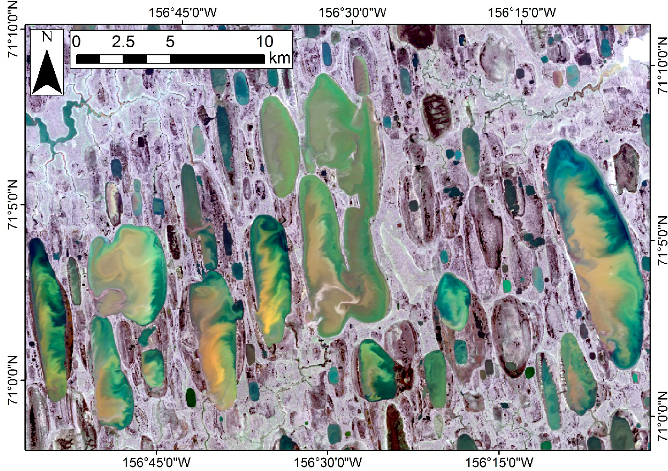
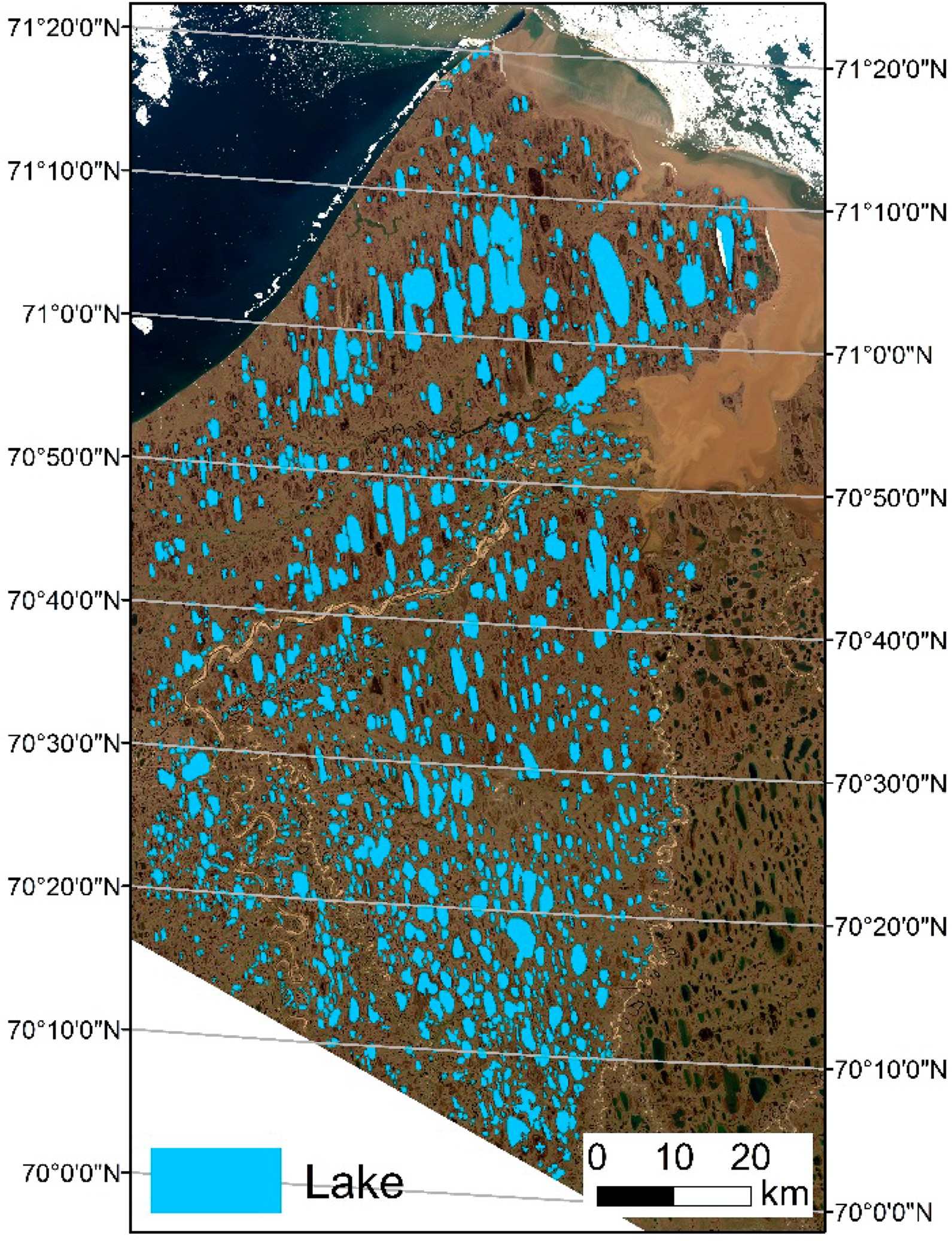
While thermokarst lakes are of great importance to climate change and the local ecosystem, the formation of elongated, oriented lakes remains controversial [11]. One of the most striking features of lakes located on the ACP of northern Alaska is that most of them are uniformly oriented in a north-south direction (Figure 1), which has been observed and studied by many researchers [12–19]. Carson and Hussey [12] documented near shore lake water circulation using dye and floats in selected lakes near Barrow, Alaska and proposed a classical theoretical model of thermokarst lake orientation in terms of wind-driven circulation and wave activity. The model explains that the prevailing winds approximately perpendicular to the axis of lake orientation carry and redistribute sediment towards the west and east shores to form protective littoral shelves while the north and south shores are preferentially eroded by thermomechanical processes. This leads to a preferred longitudinal expansion of the lakes and causes the orientation. In contrast, Pelletier [13] proposed an alternative model that explains the orientation in terms of thaw slumping of shores controlled by the local topographic aspect, slope and sun angle rather than wind condition. The veracity and regional applicability of Pelletier’s hypothesis has been analyzed by Hinkel [20]. The cause of orientation is closely related to the expansion of thermokarst lakes which can potentially affect the carbon cycle as well as the underlying permafrost. Therefore, differentiating between these two very different models for oriented thermokarst lake formation is important with regard to predicting the effect of observed climate change [21,22] on lake dynamics and the carbon-rich permafrost in which they develop.
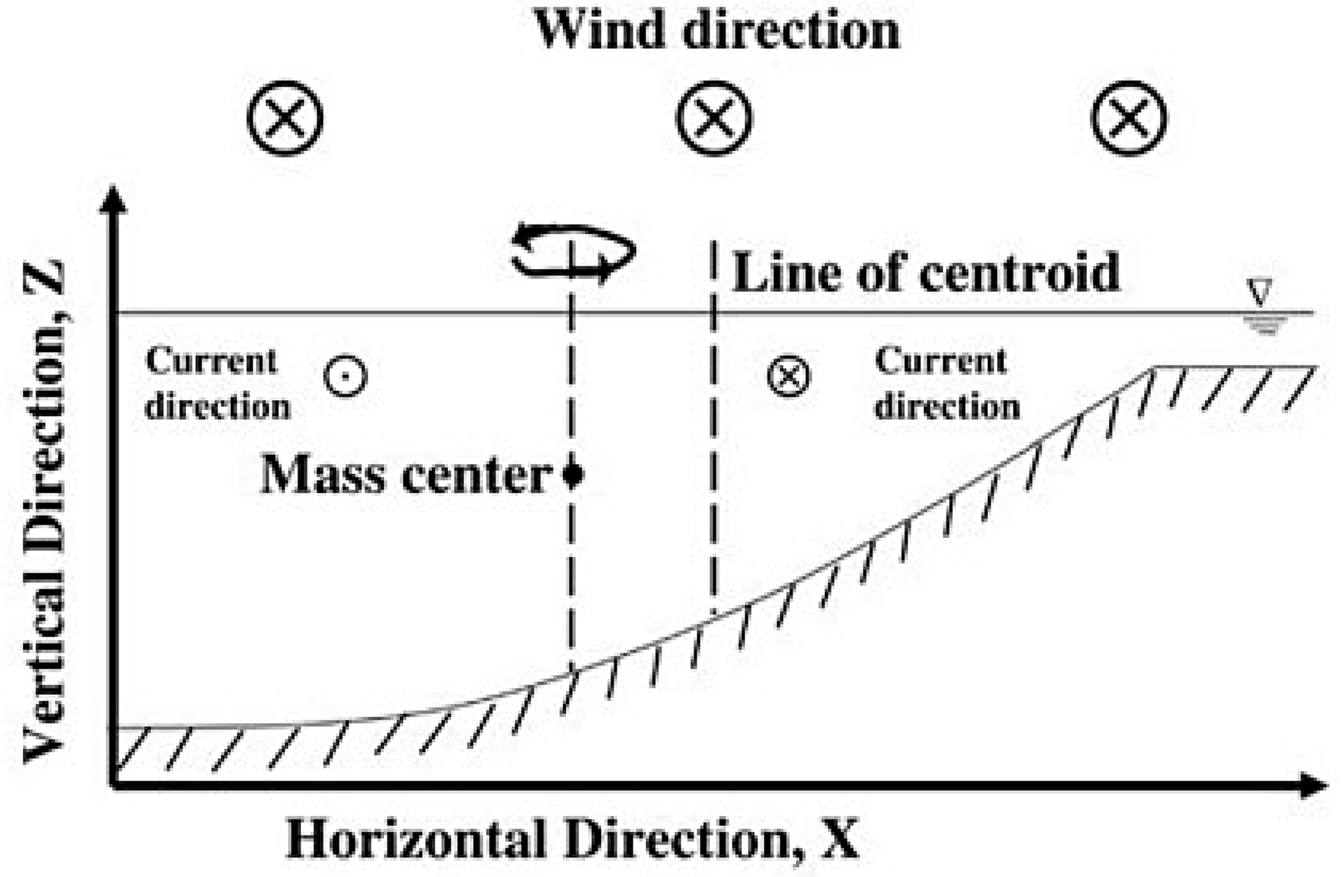
Examination of a Landsat 8 satellite image reveals a number of gyres within the thermokarst lakes on the ACP of northern Alaska (Figure 1). Gyres are rotational circulation patterns often found in lakes and oceans that are generated by winds or other physical processes. Gyres can erode lake shores, re-suspend and redistribute eroded sediment. They also play a potentially important role in the formation processes of thermokarst lakes on the ACP of northern Alaska. When wind blows into the cross-section of a lake, the wind’s line of action is through the line of the lake centroid (Figure 2). In the case of shallower water on the right and deeper water on the left, the mass center of the water body is shifted towards the deeper (left) part of the lake. Thus, a torque is produced which makes water in the shallower part flow into the cross-section and water in the deeper part flow out of the cross-section, making the water rotate. Under the predominant east-northeast winds on the ACP, clockwise (CW) gyres are expected to form near the south shores and anticlockwise (ACW) gyres are expected to form near the north shores in concordance with the gyre formation processes. To date, most studies on lake gyres have been done using in situ measurements [23,24] or model simulation [25] and focus on a single lake. No studies have been found using satellite imagery to study lake gyres on a regional scale especially on the ACP. Satellite remote sensing provides frequently repeated imagery of various spatial scale and resolution on the ACP, which is especially useful due to the limited accessibility of the region. Satellite imagery is especially favored over field measurements for studying large scale (kilometers wide) gyre occurrences because the formation and structure of gyres are difficult to describe using buoy stations or research vessels in the field [26].
This study investigates the spatial and temporal distribution of gyres in the oriented thermokarst lakes on the ACP of northern Alaska using satellite imagery and wind data. The goal of this study is to: (1) examine the spatial and temporal distribution of gyres within the entire study area as well as within individual lakes; and (2) compare the distribution pattern of gyres with the predictions of Carson and Hussey [12]. The hypotheses are: (1) wind-driven gyres on the ACP are common due to the persistent surface winds; (2) there is a decreasing trend in the number of gyre occurrences from the coastal area inland related to the changing geomorphology and decreasing lake size and wind velocity landward; (3) clockwise (CW) gyres form preferentially near the south shores of the lakes and anti-clockwise (ACW) gyres form near the north shores of the lakes during strong dominant winds from east-northeast; and (4) Gyre occurrence is highly correlated with wind speed and direction. This study reveals the widespread occurrence of wind generated gyres with the potential to shape uniformly oriented thermokarst lakes.
2. Study Area
The North Slope of Alaska is a foreland basin north of the Brooks Range [27] and includes the Arctic Foothills and the ACP. The boundary between the Foothills and the ACP is identified by a sharp break in surface slope at 120–200 m above sea level (asl). A prominent ancient shoreline at 23–29 m asl divides the ACP into a northern part of flat Outer Coastal Plain (OCP) composed of surficial marine silt and sand and a southern part of the Inner Coastal Plain (ICP) with rolling topography composed of aeolian sand and silt [28,29]. The ACP has low elevation and relief and is characterized by tens of thousands of oriented thermokarst lakes developed atop of 300–600 meter-deep permafrost.
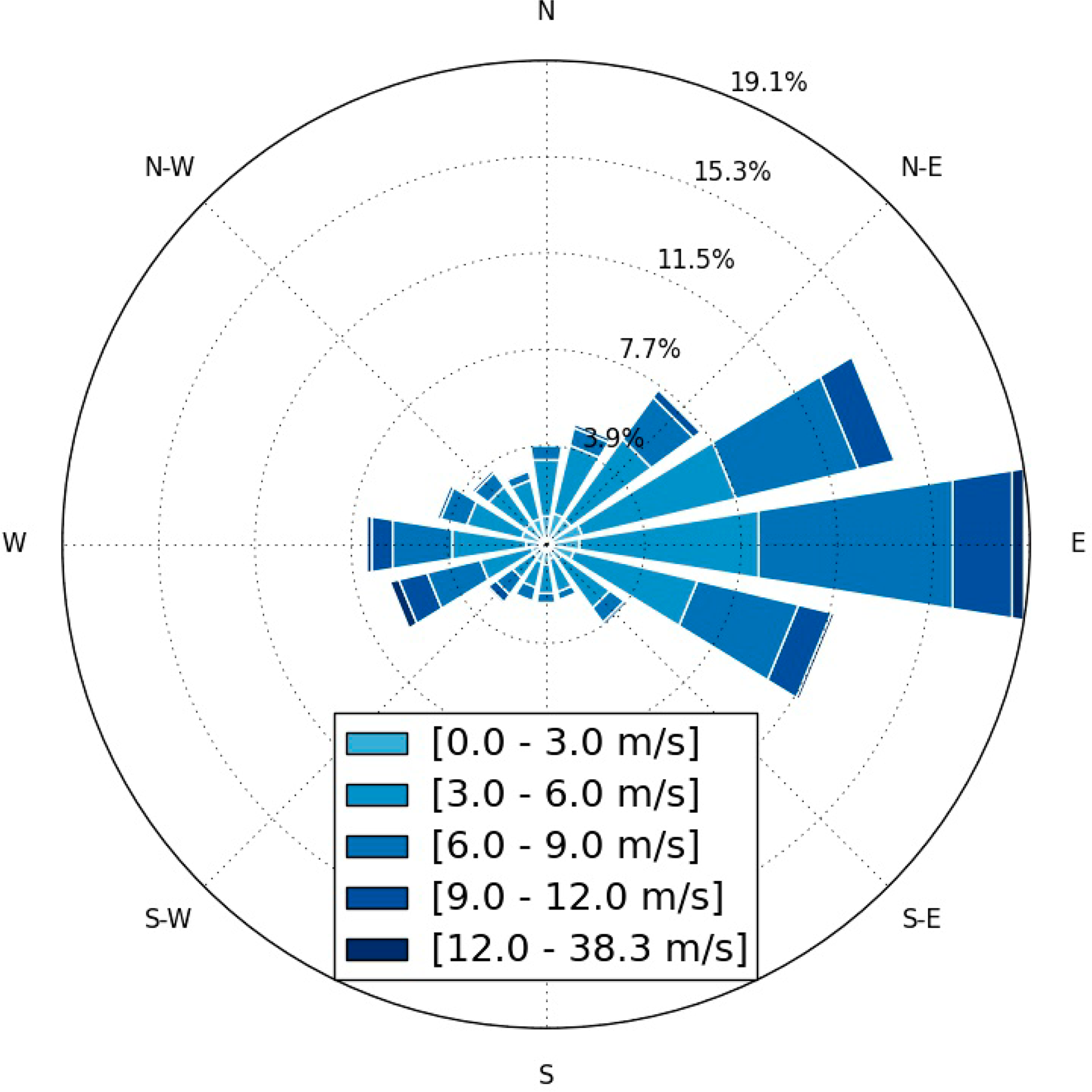
Thermokarst lakes on the ACP are frozen most of the year and are only ice-free during the summer usually from July to September. The predominant winds in the Barrow region come from east to northeast with an average speed of approximately 4–6 m per second throughout the year with less common winds from the opposite west to southwest [30,31]. Figure 3 shows the dominant bimodal (east and west) summer wind in Barrow, Alaska from 1 June to 30 September 2013. Waves and currents in these lakes are most likely to be driven by summer winds as the lakes are small and shallow and lake water largely isothermal during the ice-free season [32]. The mean depth of more than 20 lakes on the western OCP and ICP measured by Hinkel et al. [33] ranges from 1–2 m with the maximum depth rarely over 5 m. Lakes on the OCP near Barrow have flat bottoms and no well-developed littoral shelves while lakes on the ICP have varying bottom topography and prominent littoral shelves [33]. Waves generated by winds induce shear stress on the lake bottom and stir up the uppermost layer of sediment [34] and exert thermomechanical forcings on lake shores. The sediment is redistributed over the shallow lake [35] resulting in very little bottom topography in lakes on the OCP [36].
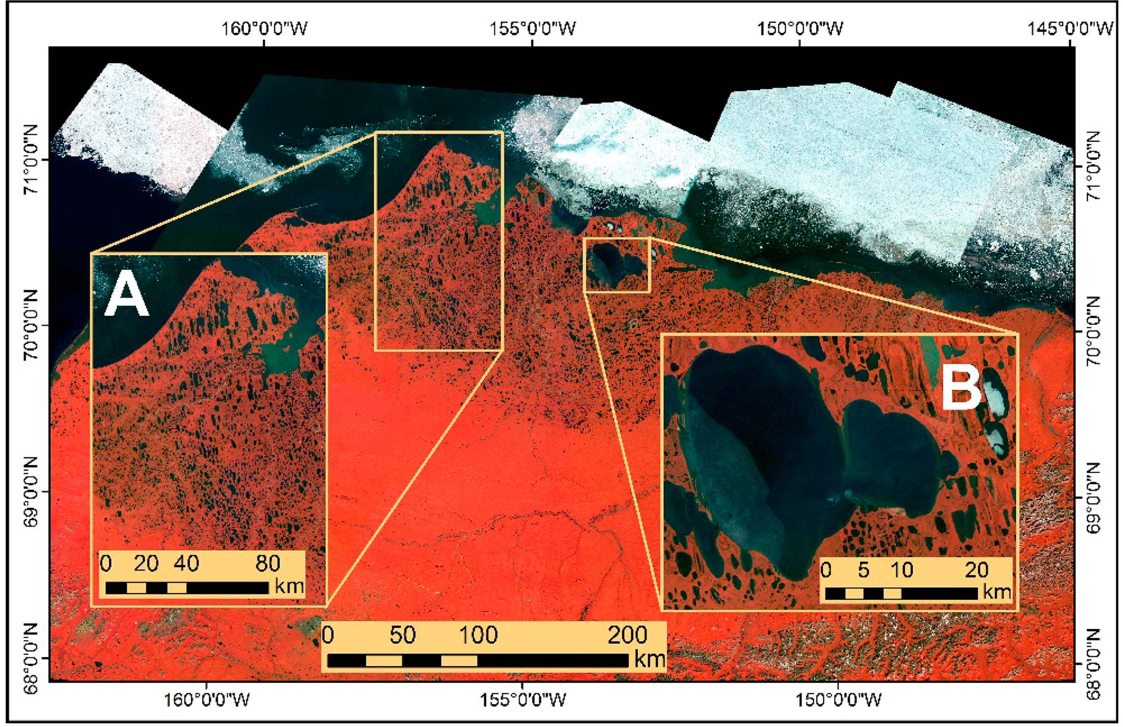
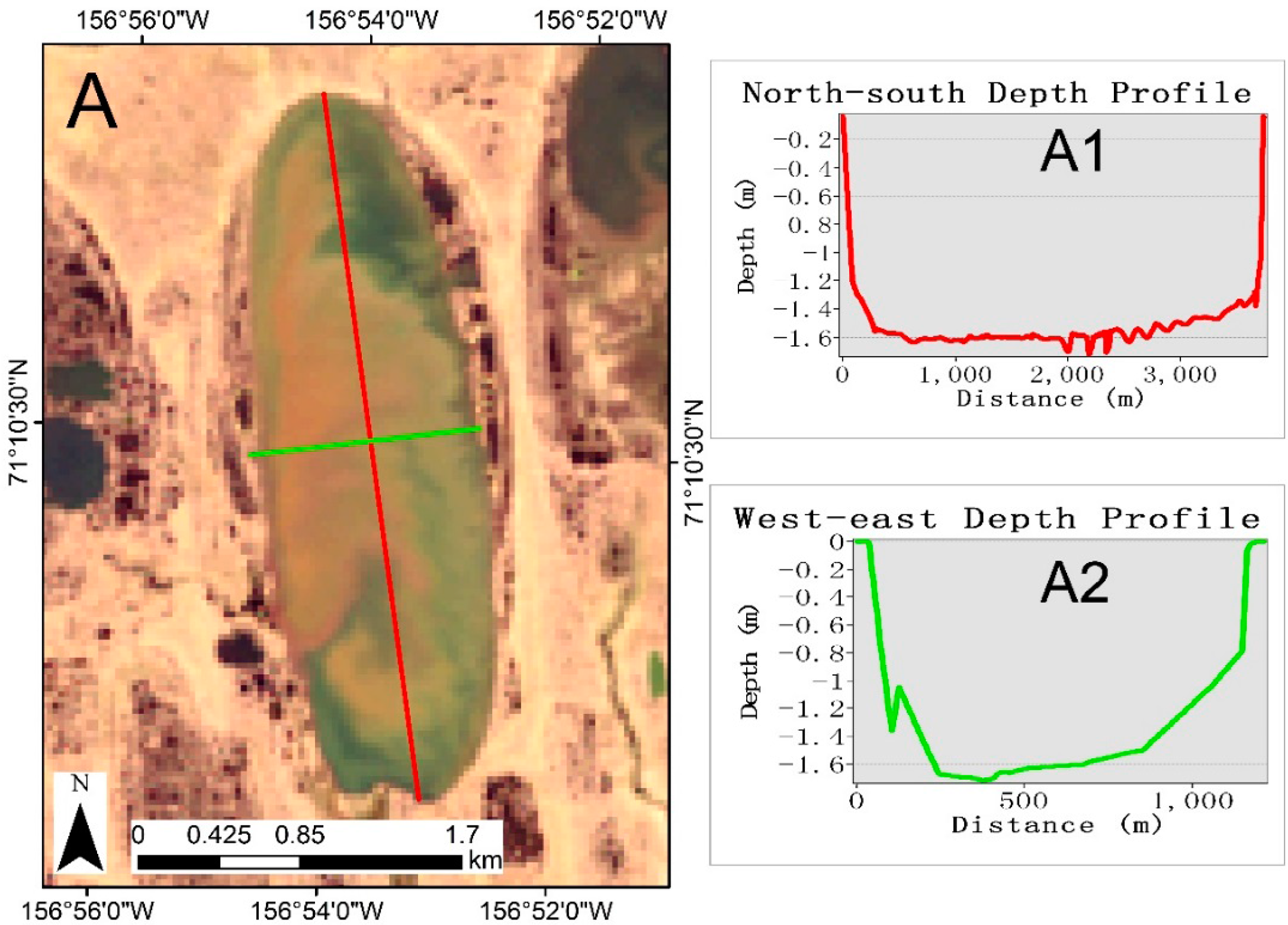
Figure 4 shows a false color composite image map of the ACP of northern Alaska. Two separate regions on the ACP were selected for this study. The first study area (Figure 4 inset map A) lies near Barrow, Alaska. The northern part of this study area lies on the OCP and southern part lies on the ICP. This study area includes over 1500 lakes (water bodies with area > 0.1 km2) of various sizes. The ice-free season for lakes in this region usually starts in late June and ends in early October. Table 1 shows the basic characteristics of these lakes [18]. Figure 5 shows field-based sonar-derived depth profiles in two cross-sections of two sample lakes on the OCP of Barrow study area. There is a great rate of descent near lake shores and most of the bottom area of the two lakes is relatively flat with little variation [33]. Thus, gyre patterns are due to suspended sediment rather than variation in bathymetry.
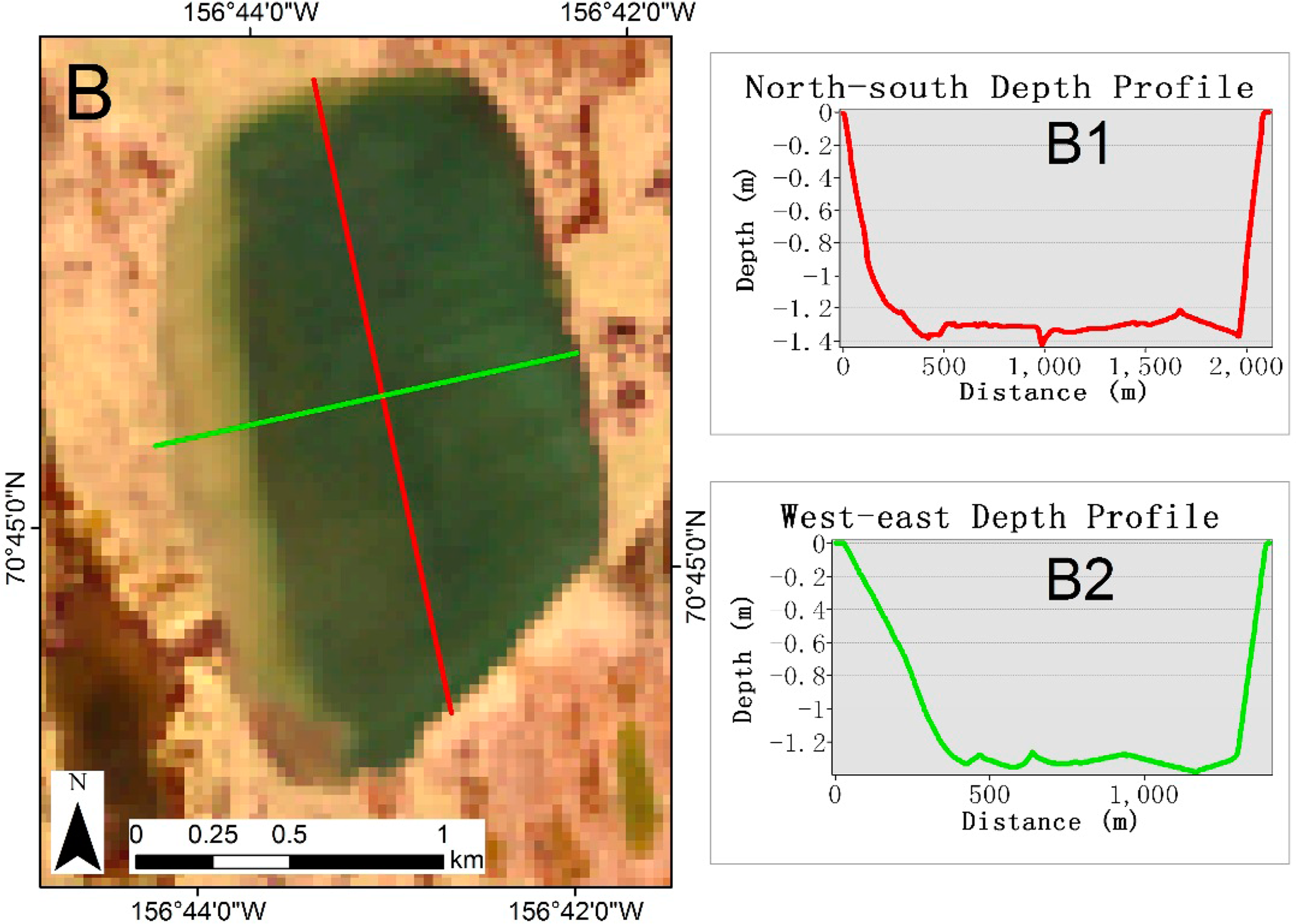
The second study area (Figure 4 inset map B) focuses on Teshekpuk Lake, which is the largest lake on the ACP. Teshekpuk Lake is located 150 km southeast of Barrow, Alaska on the boundary between the outer and inner portions of the ACP. Teshekpuk Lake is likely of a varied origin and represents the coalescence of several oriented thermokarst lake basins. Table 2 shows the basic characteristics of Teshekpuk Lake and Figure 6 shows its depth profile in a northwest-southeast direction cross-section. Similar to the smaller lakes in the Barrow study area, the bottom of Teshekpuk Lake is also relatively flat. Thus, gyre patterns are due to suspended sediment rather than variation in bathymetry. Ice in Teshekpuk Lake usually starts to melt in June and the ice-free season usually starts in mid-July and ends in early October.
3. Methods
3.1. Datasets
Fifty-two satellite images from the Landsat image archive as well as the Advanced Spaceborne Thermal Emission and Reflection Radiometer (ASTER) image archive were collected from the U.S. Geological Survey (USGS) EarthExplorer. WorldView-1 images were obtained via NASA. All of the images were collected in July, August or September when the lake surfaces were partially or completely ice-free. Table 3 shows the number of scenes and the temporal coverage of the satellite imagery used in this study. The temporal resolution of Landsat and ASTER images is 16 days. Due to the overlap between two adjacent scenes, some particular regions on average have a Landsat image every week. Barrow is also one of the cloudiest places on Earth, being 100% overcast slightly more than 50% of the year [30]. The usability of the images were highly dependent upon the cloud cover of the region which is a major constraint of this study. Teshekpuk Lake was partially covered by ice in some of the images.
Meteorological datasets were collected from meteorological stations located in Barrow, Alaska and east and north of Teshekpuk Lake. The meteorological station in Barrow was established by the National Oceanic and Atmospheric Administration (NOAA). Data collected from this station covers from 1973 to 2013 and consists of hourly-averaged wind speed and wind direction. This dataset was used for the Barrow study area. The stations at the east and north of Teshekpuk Lake were established by USGS (data courtesy of the Teshekpuk Lake Observatory). Data collected from east of Teshekpuk Lake covers from 2004 to 2013 [36] and data collected from north of Teshekpuk Lake covers from 2012 to 2013. Both datasets consist of hourly-averaged wind speed and wind direction. These two datasets were used for the Teshekpuk Lake study area.
3.2. Methods
3.2.1. Identification of Gyres
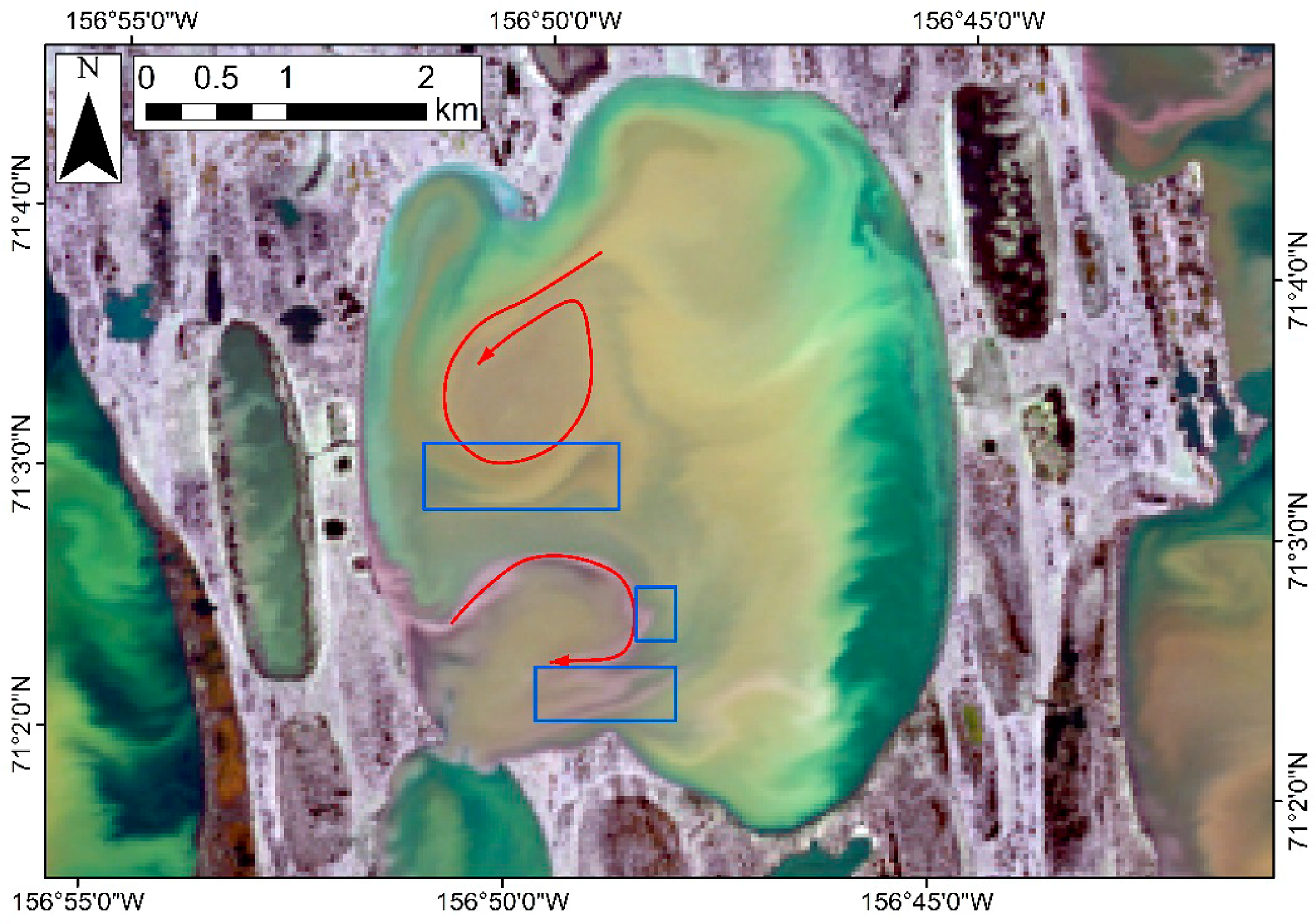
Gyres in the thermokarst lakes were identified manually from satellite images. The band combination used to identify gyres is natural color (i.e., bands 3, 2, 1 for Landsat 7 and bands 4, 3, 2 for Landsat 8). The images were enhanced for better identification of gyres. The ad hoc definition of a gyre used for identification is that a single current or a group currents has to bend at least 180° and spiral into itself/themselves. They are identified through currents that carry sediments which usually show as brighter, light-colored (brown, yellow or white) features in contrast to the darker background of clearer water. The currents in a gyre flow from the perimeter towards the center (Figure 7). Currents outside the gyre is usually more “rugged” while it appears more “smooth” inside the gyre as shown in the blue boxes in Figure 7. Thus, the direction of a gyre can be identified and the direction was recorded as CW or ACW. The successful identification of gyres with the visible spectrum imagery used here depended upon the presence of suspended sediment and its contrast against clear water.
Due to the limited radiometric resolution of the predecessors of Landsat 8, few or no gyres could be identified in the smaller lakes in the Barrow study area. Thus, only Landsat 8 images from 2013 were used to identify gyres in the Barrow study area. All available images (1999–2013) for the Teshekpuk Lake study were used to identify gyres owing the large size of Teshekpuk Lake and the ability to detect gyres across the image archive. Therefore, the spatial analysis of gyres was focused in Barrow study area while the temporal analysis mainly in Teshekpuk study area.
3.2.2. Spatial Distribution of Gyres
The Barrow study area was divided into 8 bins of 10-min latitudinal intervals (Figure 8). The number of gyres that fell into each bin was recorded and divided by the total number of lakes in that bin to derive a gyre density metric. This metric was then used to detect and measure spatial trends of gyre occurrence in the north-south direction across the entire study area.
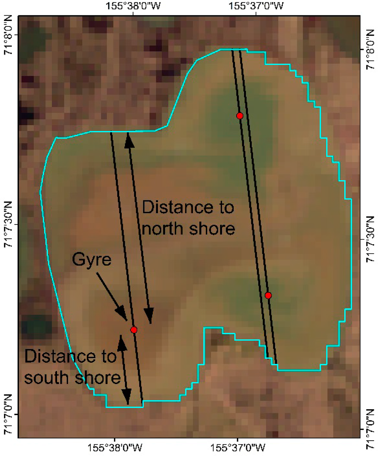
The distance of each gyre centroid along the long axis of the lake in which it lies to the north and south shores was also measured (Figure 9). The distance to the north and south shores were expressed as a fraction of the total length of the axis. The distance of CW and ACW gyres to the north and south shores of the lakes were compared using analysis of variance (ANOVA) to evaluate the difference in the location of CW and ACW gyres within each lake.
3.2.3. Temporal Distribution of Gyres
Time-series data of wind speed and wind direction during the summer when lakes are partially or completely ice-free were plotted for the imagery used in the Barrow and Teshekpuk study areas. Wind data collected by NOAA from Barrow was plotted from 1 June to 30 September in 2013. Similarly, wind data collected by the USGS from east and north Teshekpuk Lake from 1 June to 30 September each year from 2006 to 2013 were also plotted at hourly intervals. The only exception was 2011 when the wind was plotted from 1 June to 31 July due to limited data availability. Hourly wind data were represented by arrows whose direction corresponds to the wind direction and length corresponds to the magnitude of wind.
The number of gyres identified in each image was also indicated in the plots with respect to the time of image acquisition as well as the wind speed at the time of acquisition. These time-series plots were used to measure the temporal occurrence of gyres in the context of the local wind regime.
4. Results and Discussion
Seventy-two gyres were identified in both large and small thermokarst lakes in the Barrow study area from a Landsat 8 scene taken on 10 July 2013. Table 4 shows the number of gyres found per lake and Table 5 shows the number of gyres found in lakes of various sizes by quintiles. Most lakes have a single gyre while some have multiple gyres. The number of gyres found appears to be increasing with the size of the lakes in the Barrow study area.
One hundred and eleven gyres have been identified in Teshekpuk Lake from images taken between 1999 and 2013. Table 6 shows the number of gyres identified each year from 1999 to 2013. On average, 2.1 images per year can be found with gyres, each image contains 3.5 gyres and 62.7% of the images contain gyres.
4.1. Spatial Distribution of Gyres across the ACP
The 72 gyres, the largest number of gyres that have been identified from a single scene, identified in the Barrow study area from a Landsat 8 scene taken on 10 July 2013 were distributed across 50 lakes. Figure 10a shows the spatial distribution of the identified gyres. Figure 10b shows the histogram of the number of gyres in each 10-min latitude bin and Figure 10c shows the histogram of gyre density in each bin. It can be seen that there is a decreasing number of gyres in the north-south direction. The small amount of gyres found in the uppermost bin is likely due to the smaller size of lakes as they have smaller wind fetch. In addition, the northern most lakes are most influenced by human activities and they experience anthropogenic drainage in addition to natural drainage. This decrease in the number of gyres from north to south partly corresponds to a decrease in wind energy from the coast towards inland [37]. In addition, the marine silt that underlies lakes on the OCP (north) is more susceptible to entrainment by currents while the aeolian sand that underlies lakes on the ICP (south) is less susceptible to entrainment. Thus, more gyres tend to be detectable in lakes on the OCP from satellite images and we may have underestimated their occurrence inland.
4.2. Locational Difference of Clockwise and Anticlockwise Gyres within Lakes
The locational differences of the 72 gyres in the lakes in the Barrow study area and a total of 111 gyres found from images spanning from 1999 to 2013 in Teshekpuk Lake study area were examined. Table 5 shows the statistics of the locational differences of CW and ACW gyres within lakes in Barrow study area, while Table 6 shows the statistics of the locational differences of CW and ACW gyres within Teshekpuk Lake study area. The distance values were standardized by the length of the long axis across each gyre. The distance value starts at 0 on the south shore and reaches 1 on the north shore.
For the Barrow study area (Table 7), CW gyres were preferentially located towards the southern end of the lakes and while ACW gyres were preferentially located near the center of the lakes they were nonetheless located north relative to CW ones. The difference between the locations of CW and ACW gyres are statistically significant. This locational difference of CW and ACW gyres corresponds well to the formation mechanism of gyres when there is relatively constant wind blowing from one direction (wind data shown in the next section).
For the Teshekpuk Lake study area (Table 8), while CW gyres on average still occur south relative to ACW gyres, there is no significant difference between the location of CW and ACW gyres. A possible explanation for the non-significant difference in gyre location with respect to gyre direction in Teshekpuk Lake is that the 111 gyres were identified from images taken at different times from 1999 to 2013 and the wind regime during the time each image was taken was different. Because wind direction in this region is bimodal, when wind blows from west to south-west direction the location of CW and ACW gyres will tend to switch. Nevertheless, the fact that CW gyres were on average distributed towards the southern half of the lake somewhat reflects the predominant east to north-east wind regime.
4.3. Temporal Distribution of Gyres
Figure 11 shows the time-series of wind data collected at Barrow from 1 June to 30 September 2013. The blue line shows the hourly series of wind speed and the black arrows represent wind direction and magnitude at each hourly sampling point. Four Landsat 8 scenes fall into this time period and the number of gyres in each scene (4, 10, 72 and 1) are indicated in the plot. It can be seen that wind speed was steadily increasing starting from 6 July to a peak on 15 July. The number of gyres was also increasing from 10 (8 July) and 72 (10 July). Wind direction during this time period shifted from east-southeast to north-east and to east-northeast. Similar behavior has been observed on Lake Onega in Russia with a double-gyre circulation system forming after a few hours of steady moderate wind forcing and persisting for days during calm intervals [26].
Figure 12 shows the time-series of wind data collected near Teshekpuk Lake from June to September each year from 2006 to 2013. The time-series started on 1 June and ended on 30 September in all years except for 2011 which ended on 31 July. Gyres have been found in 28 usable images from 2006 to 2011. On average, 3.5 images each year can be found that have gyres in Teshekpuk Lake and each image contains 2.7 gyres.
There does not seem to be a simple correlation between the occurrence of gyres and wind speed. While there was increasing number of gyres with increasing wind speed shown in Figure 11, 11 gyres were identified on 15 September 2009 (Figure 12) with winds of less than 4 m/s and varying directions for several days beforehand. There was steady strong wind whose direction gradually shifted from north-west to west from 25 September to 29 September but only one gyre was identified in a scene taken on 28 September 2010 (Figure 12). Similarly, there was relatively strong wind coming consistently from east-northeast from 12 August to 16 August but only one gyre was identified on 16 August 2008 (Figure 12). In 2013, three scenes on Teshekpuk Lake have also been found to have increasing number of gyres from 10 to 12 July 2013 (Figure 12) under similar wind conditions from 6 to 15 July shown in the Barrow wind time series (Figure 11). Note however, that the wind speed was slightly decreasing while the number of gyres was increasing. A possible explanation for the observed patterns is the time lag between the exertion of wind force and the formation of gyres of varying sizes and the likelihood of a variety of circulation patterns and energy states as seen on Lakes Onega and Ladoga [26]. It takes time and relatively stable wind direction to accumulate enough energy on the water surface for currents to form an identifiable shape like a gyre. When wind direction changes, the direction of currents changes and thus currents may not form the shape of a gyre even though there is a great amount of turbulence in the lake (Figure 2). It also takes time for currents to settle after the wind calms down and new gyres may still form due to the momentum of the water. The Coriolis effect may also complicate the circulation patterns in these high latitude lakes.
4.4. Discussion
4.4.1. Limitations in Gyre Identification
There is a certain amount of subjectivity in the process of gyre identification as each gyre takes a somewhat different form. The lower radiometric resolution of the Landsat images prior to Landsat 8 also makes the process more subjective and prone to error. This limitation can be partly overcome by using a test group of interpreters to support the identification process which has been done in [38] or using a (semi-) automatic algorithm to detect gyres and conduct accuracy assessment on the results. The successful identification of gyres is also dependent upon the presence of suspended sediments which partly explains the fewer number of gyres found towards the southern part of Barrow study area. Nevertheless, the purpose of this study is to reveal the wide occurrence of gyres both spatially and temporally and results have shown evidence to support the model of Carson and Hussey [12].
4.4.2. Implications on Lake Formation and Evolution
The frequent documentation and existence of gyres fulfills a necessary condition for the wind-driven wave-cut theory of thermokarst lake orientation formation proposed by Carson and Hussey [12]. The locational difference of CW and ACW gyres indicates that the gyres are wind-driven and follow the lake gyre formation mechanism discussed in Ji and Jin [25] and corresponds well to the water circulation systems in the lakes under certain wind regimes discussed in Carson and Hussey [12]. Figures 13 and 15 show the comparison of between the observed current flow pattern and the qualitative water circulation analysis from Carson and Hussey [12] in Ikroavik Lake, Loon Lake and Gull Lake.
All three lakes are located near Barrow, Alaska. Under similar wind conditions, the observed current flows in Ikroavik Lake and Gull Lake (Figures 13 and 14) are reasonably comparable to the theoretical model, though the observed currents are naturally more complicated. The wind direction at Loon Lake (Figure 15) during the WorldView overpass was slightly different from that when Carson and Hussey [12] conducted their measurements (east-southeast vs. east), but nonetheless resulted in a CW gyre near south shore and an ACW gyre near north shore. The different spatial location of CW and ACW gyres indicates that there are preferential locations where gyres tend to form (i.e., near north and south shores) under the prevailing wind regime. These near-shore current activities may promote erosion of north and south shores over time, which may ultimately lead to thermokarst lake elongation and orientation that is observed today. The ability of gyres to resuspend and redistribute sediment may also help to explain the flat bottom found in many of the lakes on the ACP [33].
Oriented lakes are also found in the Bolivian Amazon and recent study has found that their orientation may also have been caused by wind-driven water circulations in combination with other mechanism [39]. While the major wind direction in the Bolivian Amazon in relation to lake orientation is different from that of the ACP [39], it would be interesting to see whether Carson and Hussey’s model can explain the orientation of lakes in this region.
4.4.3. Implications for Changing Northern High Latitude Ecosystems
Given amplification of climate change in the Arctic, lakes tend to experience a longer ice-free period during the summer months. The horizontal and vertical mixing ability of wind-driven gyres in part contributes to the largely isothermal lakes during the summer as documented by Hinkel et al., [32]. Surdu et al., [8] have found a later ice onset by 5.9 days, a significant advancement of ice melt by 17.7 to 18.6 days and a decrease in the ice season by 23.6 to 24.8 days in the lakes near Barrow, Alaska from 1950 to 2011 using model simulations. Hinkel et al., [40] observed notable interannual differences in lake ice melt out near Barrow, Alaska and suggested a strong influence from nearshore marine conditions. Wendler et al. [31] attribute an 18% increase in wind speeds measured along the ACP to a decline in sea ice extent. In addition, the average number of storms was estimated to increase from four to ten per year between 1972 and 2007 [31]. Should the lake ice season continue to decrease, combined with an increase in wind speeds and storm events, it will allow for the development of more gyres in the lakes, which may lead to an accelerated longitudinal expansion of the lakes. This in turn could increase the rate at which thermokarst lakes expand through thermomechanical erosion and lead to an increase in the surface area of lakes. Alternatively, this could also result in a decrease in the surface area of lakes if the increased lake expansion promotes catastrophic drainage.
5. Conclusions
This study is the first to examine the regional spatial and temporal distribution of gyres in the oriented thermokarst lakes on the Arctic Coastal Plain (ACP) of northern Alaska. Gyres were studied in terms of latitude, lake size and distance to shore metrics using satellite imagery and meteorological data. Over 150 gyres were manually identified in 51 lakes from over 50 satellite images spanning the period 1999 to 2013. Results show the widespread and frequent occurrence of gyres in thermokarst lakes on the ACP following sustained winds, usually from the east to northeast, supporting the wind-driven gyre hypothesis of Carson and Hussey [12]. Decades of meteorological data confirm the year round frequency and directional consistency of strong winds and frequently overcast conditions on the ACP especially during the summer ice-free season. The widespread and frequent occurrence of gyres and the climate of the ACP generally supports the wind-driven gyre hypothesis of Carson and Hussey [12] as opposed to the recent solar insolation/topography origin proposed by Pelletier [13] for the oriented thermokarst lakes of the region.
Within this overall windy and overcast climate, 32 out of 47 images of Teshekpuk Lake showed the presence of gyres. However, there is no simple correlation between the number of gyres in Teshekpuk Lake and wind speed. This is possibly due to a time lag between wind forcing and gyre formation as well as complex circulation patterns and energy states driven by forces other than wind. There is a decreasing occurrence and density of gyres inland away from the Arctic Ocean, likely corresponding to a decrease in wind energy away from the coast as well as morphological changes in the underlying sedimentology. Under a steady moderate east-northeast wind regime, a statistically significant difference (p-value < 0.01) in the location between clockwise (CW) and anti-clockwise (ACW) gyres has been found. CW gyres tend to form near the south shore of lakes and ACW gyres are on average located near the center of the lake but nonetheless further north relative to CW gyres. This observation corresponds well to the gyre formation theory.
The observed spatial pattern of gyres and currents within lakes from satellite imagery corresponds well with the field observations documented by Carson and Hussey [12]. Observations from this study fulfill a necessary condition of the wind-driven, wave-cut model of oriented thermokarst lake development on the ACP. It also suggests that thermokarst lakes will continue to expand in the north-south direction. The oriented thermokarst lakes on the ACP of northern Alaska are experiencing longer ice-free periods during the summer and an increased wind regime in a changing climate, which will allow more gyre development and potentially an increase in erosion and expansion of north and south shores. This increase has implications for changes in northern high latitude aquatic ecosystems, particularly if wind-generated gyres promote permafrost degradation and thermokarst lake expansion.
Acknowledgments
This study was funded in part by NSF AON grant 107607. Any use of trade, product, or firm names is for descriptive purposes only and does not imply endorsement by the USA Government.
Author Contributions
Shengan Zhan contributed the study design, overall analysis, and manuscript writing. Richard A. Beck, Kenneth M. Hinkel and Benjamin M. Jones contributed field data, analysis and manuscript editing. Hongxing Liu contributed field data.
Conflicts of Interest
The authors declare no conflict of interest.
References
- Walter, K.M.; Edwards, M.E.; Grosse, G.; Zimov, S.A.; Chapin, F.S. Thermokarst lakes as a source of atmospheric CH4 during the last deglaciation. Science 2007, 318, 633–636. [Google Scholar]
- Edwards, M.; Walter, K.; Grosse, G.; Plug, L.; Slater, L.; Valdes, P. Arctic thermokarst lakes and the carbon cycle. Science 2009, 17, 16–18. [Google Scholar]
- Walter, K.M.; Zimov, S.A.; Chanton, J.P.; Verbyla, D.; Chapin, F.S. Methane bubbling from Siberian thaw lakes as a positive feedback to climate warming. Nature 2006, 443, 71–75. [Google Scholar]
- Schuur, E.A.G.; Abbott, B.W.; Bowden, W.B.; Brovkin, V.; Camill, P.; Canadell, J.G.; Chanton, J.P.; Chapin, F.S., III; Christensen, T.R.; Ciais, P.; et al. Expert assessment of vulnerability of permafrost carbon to climate change. Clim. Chang 2013, 119, 359–374. [Google Scholar]
- Harden, J.W.; Koven, C.D.; Ping, C.-L.; Hugelius, G.; David McGuire, A.; Camill, P.; Grosse, G. Field information links permafrost carbon to physical vulnerabilities of thawing. Geophys. Res. Lett 2012, 39, L15704. [Google Scholar]
- Schuur, E.A.G.; Bockheim, J.; Canadell, J.G.; Euskirchen, E.; Field, C.B.; Goryachkin, S.V.; Hagemann, S.; Kuhry, P.; Lafleur, P.M.; Lee, H.; et al. Vulnerability of permafrost carbon to climate change: Implications for the global carbon cycle. BioScience 2008, 58, 701–714. [Google Scholar]
- Arp, C.D.; Jones, B.M.; Lu, Z.; Whitman, M.S. Shifting balance of thermokarst lake ice regimes across the Arctic Coastal Plain of northern Alaska. Geophys. Res. Lett 2012, 39, L16503. [Google Scholar]
- Surdu, C.M.; Duguay, C.R.; Brown, L.C.; Prieto, D.F. Response of ice cover on shallow lakes of the North Slope of Alaska to contemporary climate conditions (1950–2011): Radar remote-sensing and numerical modeling data analysis. Cryosphere 2014, 8, 167–180. [Google Scholar]
- Jones, B.M.; Arp, C.D.; Hinkel, K.M.; Beck, R.A.; Schmutz, J.A.; Winston, B. Arctic lake physical processes and regimes with implications for winter water availability and management in the National Petroleum Reserve Alaska. Environ. Manag 2009, 43, 1071–1084. [Google Scholar]
- Arp, C.D.; Jones, B.M.; Schmutz, J.A.; Urban, F.E.; Jorgenson, M.T. Two mechanisms of aquatic and terrestrial habitat change along an Alaskan Arctic coastline. Polar Biol 2010, 33, 1629–1640. [Google Scholar]
- Grosse, G.; Jones, B.; Arp, C. Thermokarst lakes, drainage, and drained basins. In Treatise on Geomorphology; Shroder, J., Giardino, R., Harbor, J., Eds.; Academic Press: San Diego, CA, USA, 2013; Volume 8, pp. 325–353. [Google Scholar]
- Carson, C.E.; Hussey, K.M. The oriented lakes of Arctic Alaska. J. Geol 1962, 70, 417–439. [Google Scholar]
- Pelletier, J. Formation of oriented thaw lakes by thaw slumping. J. Geophys. Res 2005, 110, F02018. [Google Scholar]
- Cote, M.M.; Burn, C.R. The Oriented lakes of Tuktoyaktuk Peninsula, Western Arctic Coast, Canada: A GIS-based Analysis. Permafr. Periglac. Process 2002, 13, 61–70. [Google Scholar]
- Black, R.F.; Barksdale, W.L. Oriented lakes of northern Alaska. J. Geol 1949, 57, 105–118. [Google Scholar]
- Livingstone, D.A. On the orientation of lake basins. Am. J. Sci 1954, 252, 547–554. [Google Scholar]
- Frohn, R.C.; Hinkel, K.M.; Eisner, W.R. Satellite remote sensing classification of thaw lakes and drained thaw lake basins on the North Slope of Alaska. Remote Sens. Environ 2005, 97, 116–126. [Google Scholar]
- Hinkel, K.M.; Frohn, R.C.; Nelson, F.E.; Eisner, W.R.; Beck, R.A. Morphometric and spatial analysis of thaw lakes and drained thaw lake basins in the western Arctic Coastal Plain, Alaska. Permafr. Periglac. Process 2005, 16, 327–341. [Google Scholar]
- Arp, C.D.; Jones, B.M.; Urban, F.E.; Grosse, G. Hydrogeomorphic processes of thermokarst lakes with grounded-ice and floating-ice regimes on the Arctic coastal plain, Alaska. Hydrol. Process 2011, 25, 2422–2438. [Google Scholar]
- Hinkel, K. Comment on “Formation of oriented thaw lakes by thaw slumping” by Jon D. Pelletier. J. Geophys. Res 2006, 111, F01021. [Google Scholar]
- Anisimov, O.A.; Vaughan, D.G.; Callaghan, T.V.; Furgal, C.; Marchant, H.; Prowse, T.D.; Vilhjálmsson, H.; Walsh, J.E. Polar regions (Arctic and Antarctic). In Climate Change 2007: Impacts, Adaptation and Vulnerability. Contribution of Working Group II to the Fourth Assessment Report of the Intergovernmental Panel on Climate Change; Parry, M.L., Canziani, O.F., Palutikof, J.P., van der Linden, P.J., Hanson, C.E., Eds.; Cambridge University Press: Cambridge, UK, 2007; pp. 653–685. [Google Scholar]
- Vaughan, D.G.; Comiso, J.C.; Allison, I.; Carrasco, J.; Kaser, G.; Kwok, R.; Mote, P.; Murray, T.; Paul, F.; Ren, J.; et al. Observations: Cryosphere. In Climate Change 2013: The Physical Science Basis. Contribution of Working Group I to the Fifth Assessment Report of the Intergovernmental Panel on Climate Change; Stocker, T.F., Qin, D., Plattner, G.-K., Tignor, M., Allen, S.K., Boschung, J., Nauels, A., Xia, Y., Bex, V., Midgley, P.M., Eds.; Cambridge University Press: Cambridge, UK/New York, NY, USA, 2013; pp. 317–382. [Google Scholar]
- Lemmin, U.; D’Adamo, N. Summertime winds and direct cyclonic circulation: Observations from Lake Geneva. Ann. Geophys 1996, 14, 1207–1220. [Google Scholar]
- Endoh, S.; Okumura, Y. Gyre system in Lake Biwa derived from recent current measurements. Jpn. J. Limnol 1993, 54, 191–197. [Google Scholar]
- Ji, Z.; Jin, K.; Circle, I.L.; Beach, W.P. Gyres and seiches in a large and shallow lake. J. Great Lakes Res 2006, 32, 764–775. [Google Scholar]
- Kondratyev, K.Y.; Filatov, N. Limnology and Remote Sensing: A Contemporary Approach; Springer: Berlin/Heidelberg, Germany, 1999; p. 285. [Google Scholar]
- Bird, K.J.; Molenaar, C.M. The North Slope foreland basin, Alaska. Foreland Basins and Fold Belts: American Association of Petroleum Geologists Memoir, Macqueen, R.W., Leckie, D.A., Eds.; Available online: http://archives.datapages.com/data/specpubs/basinar3/data/a136/a136/0001/0350/0363.htm (accessed on 23 September 2014).
- Williams, J.R.; Carter, L.D.; Yeend, W.E. Coastal plain deposits of NPRA. The United States Geological Survey in Alaska: Accomplishments during 1977, Geological Survey Circular 772-B, B-20-22. Johnson, K.M., Ed.; Available online: http://www.dggs.alaska.gov/pubs/id/13467 (accessed on 23 September 2014).
- Williams, J.R. Engineering-Geologic Maps of Northern Alaska, Meade River Quadrangle; United States Geological Survey Open-File Report 83-294. U.S. Geological Survey, 1983. Available online: http://www.dggs.alaska.gov/pubs/id/11493 (accessed on 23 September 2014).
- Maykut, P.E.; Church, G.A. Radiation climate of Barrow, Alaska, 1962–1966. J. Appl. Meteorol 1973, 12, 620–628. [Google Scholar]
- Wendler, G.; Shulski, M.; Moore, B. Changes in the climate of the Alaskan North Slope and the ice concentration of the adjacent Beaufort Sea. Theor. Appl. Climatol 2010, 99, 67–74. [Google Scholar]
- Hinkel, K.M.; Lenters, J.D.; Sheng, Y.; Lyons, E.A.; Beck, R.A.; Eisner, W.R.; Maurer, E.F.; Wang, J.; Potter, B.L. Thermokarst lakes on the Arctic Coastal Plain of Alaska: Spatial and temporal variability in summer water temperature. Permafr. Perigl. Process 2012, 23, 207–217. [Google Scholar]
- Hinkel, K.M.; Sheng, Y.; Lenters, J.D.; Lyons, E.A.; Beck, R.A.; Eisner, W.R.; Wang, J. Thermokarst lakes on the Arctic Coastal Plain of Alaska: Geomorphic controls on bathymetry. Permafr. Perigl. Process 2012, 23, 218–230. [Google Scholar]
- Józsa, J. On the internal boundary layer related wind stress curl and its role in generating shallow lake circulations. J. Hydrol. Hydromech 2014, 62, 16–23. [Google Scholar]
- Bengtsson, L. Hydrodynamics of very shallow lakes. In Encyclopedia of Lakes and Reservoirs; Bengtsson, L., Herschy, R.W., Fairbridge, R.W., Eds.; Springer: Berlin/Heidelberg, Germany, 2012; pp. 344–346. [Google Scholar]
- Urban, F.E.; Clow, G.D. DOI/GTN-P Climate and Active-Layer Data Acquired in the National Petroleum Reserve-Alaska and the Arctic National Wildlife Refuge, 1998–2011: U.G. Geological Survey Data Series 812. Available online: http://pubs.usgs.gov/ds/812/introduction.html (accessed on 24 September 2014).
- Searby, H.W.; Hunter, M. Climate of the North Slope of Alaska, NOAA Technical Memorandum AR-4, 1–53; U.S. Department of Commerce, 1971. Available online: http://docs.lib.noaa.gov/noaa_documents/NWS/TM_NWS_AR/TM_NWS_AR_4.pdf (accessed on 23 September 2014).
- Sannel, A.B.K.; Brown, I.A. High-resolution remote sensing identification of thermokarst lake dynamics in a subarctic peat plateau complex. Can. J. Remote Sens 2010, 36, S26–S40. [Google Scholar]
- Hinkel, K.M.; Lin, Z.; Sheng, Y.; Evan, A. Spatial patterns of lake ice meltout near Barrow, Alaska. Polar Geogr 2012, 35, 1–18. [Google Scholar]
- Lombardo, U.; Veit, H. The origin of oriented lakes: Evidence from the Bolivian Amazon. Geomorphology 2014, 204, 502–509. [Google Scholar]


| Number of Lakes (Area > 0.1 km2) | Mean Area (km2) | Median Area (km2) | Min. Area (km2) | Max. Area (km2) | Mean Orientation |
|---|---|---|---|---|---|
| 1511 | 0.9819 | 0.3765 | 0.1008 | 48.4154 | N10°W |
| Area (km2) | North-South Length (km) | East-West Length (km) | Orientation |
|---|---|---|---|
| 687.0587 | 32.25 | 37.03 | N15°W |
| 1999 | 2000 | 2001 | 2002 | 2003 | 2005 | 2006 | 2007 | 2008 | 2009 | 2010 | 2011 | 2012 | 2013 | |
|---|---|---|---|---|---|---|---|---|---|---|---|---|---|---|
| Landsat 4 | ||||||||||||||
| Landsat 5 | 1 | 1 | 1 | 1 | ||||||||||
| Landsat 7 | 4 | 3 | 1 | 5 | 1 | 1 | 4 | 5 | 2 | 4 | 2 | 1 | 3 | 2 |
| Landsat 8 | 4 | |||||||||||||
| ASTER | 1 | 1 | 1 | 2 | ||||||||||
| WorldView-1 | 1 |
| Number of Gyres per Lake | Number of Lakes with Gyre |
|---|---|
| 1 | 39 |
| 2 | 9 |
| 3 | 5 |
| 4 | 1 |
| Quintile | 1st | 2nd | 3rd | 4th | 5th | Total |
|---|---|---|---|---|---|---|
| Lake Size (km2) | 0.49–1.56 | 1.56–2.80 | 2.80–4.20 | 4.20–8.20 | 8.20–48.42 | |
| Number of lakes | 10 | 10 | 10 | 10 | 10 | 50 |
| Number of gyres | 11 | 14 | 14 | 17 | 16 | 72 |
| Year | 1999 | 2000 | 2002 | 2006 | 2007 | 2008 | 2009 | 2010 | 2011 | 2012 | 2013 | Total |
|---|---|---|---|---|---|---|---|---|---|---|---|---|
| Number of scenes with gyre | 3 | 3 | 3 | 4 | 4 | 1 | 2 | 3 | 1 | 2 | 6 | 32 |
| Number of gyres | 12 | 18 | 5 | 10 | 12 | 1 | 12 | 5 | 4 | 3 | 29 | 111 |
| Total number of scenes | 4 | 4 | 5 | 6 | 5 | 3 | 5 | 5 | 1 | 3 | 6 | 47 |
| Gyre Direction | Number | Mean Distance to South Shore | Standard Deviation of Mean | ANOVA F-test | ANOVA p-value |
|---|---|---|---|---|---|
| CW | 36 | 0.377 | 0.283 | 8.184 | 0.006 |
| ACW | 36 | 0.557 | 0.250 |
| Gyre Direction | Number | Mean Distance to South Shore | Standard Deviation of Mean | ANOVA F-test | ANOVA p-value |
|---|---|---|---|---|---|
| CW | 51 | 0.441 | 0.264 | 0.974 | 0.326 |
| ACW | 60 | 0.496 | 0.314 |
© 2014 by the authors; licensee MDPI, Basel, Switzerland This article is an open access article distributed under the terms and conditions of the Creative Commons Attribution license (http://creativecommons.org/licenses/by/4.0/).
Share and Cite
Zhan, S.; Beck, R.A.; Hinkel, K.M.; Liu, H.; Jones, B.M. Spatio-Temporal Analysis of Gyres in Oriented Lakes on the Arctic Coastal Plain of Northern Alaska Based on Remotely Sensed Images. Remote Sens. 2014, 6, 9170-9193. https://doi.org/10.3390/rs6109170
Zhan S, Beck RA, Hinkel KM, Liu H, Jones BM. Spatio-Temporal Analysis of Gyres in Oriented Lakes on the Arctic Coastal Plain of Northern Alaska Based on Remotely Sensed Images. Remote Sensing. 2014; 6(10):9170-9193. https://doi.org/10.3390/rs6109170
Chicago/Turabian StyleZhan, Shengan, Richard A. Beck, Kenneth M. Hinkel, Hongxing Liu, and Benjamin M. Jones. 2014. "Spatio-Temporal Analysis of Gyres in Oriented Lakes on the Arctic Coastal Plain of Northern Alaska Based on Remotely Sensed Images" Remote Sensing 6, no. 10: 9170-9193. https://doi.org/10.3390/rs6109170