Water Level Fluctuations in the Congo Basin Derived from ENVISAT Satellite Altimetry


Abstract
: In the Congo Basin, the elevated vulnerability of food security and the water supply implies that sustainable development strategies must incorporate the effects of climate change on hydrological regimes. However, the lack of observational hydro-climatic data over the past decades strongly limits the number of studies investigating the effects of climate change in the Congo Basin. We present the largest altimetry-based dataset of water levels ever constituted over the entire Congo Basin. This dataset of water levels illuminates the hydrological regimes of various tributaries of the Congo River. A total of 140 water level time series are extracted using ENVISAT altimetry over the period of 2003 to 2009. To improve the understanding of the physical phenomena dominating the region, we perform a K-means cluster analysis of the altimeter-derived river level height variations to identify groups of hydrologically similar catchments. This analysis reveals nine distinct hydrological regions. The proposed regionalization scheme is validated and therefore considered reliable for estimating monthly water level variations in the Congo Basin. This result confirms the potential of satellite altimetry in monitoring spatio-temporal water level variations as a promising and unprecedented means for improved representation of the hydrologic characteristics in large ungauged river basins.1. Introduction
Despite the global importance of the Congo Basin, which is the second largest river basin in the world, only a small number of studies to date have focused on the potential impact of climate change on the hydro-climatic variability over the Congo Basin using in situ data and/or hydrological models. The limited understanding of climate dynamics in the Congo Basin is in part due to the lack of the in situ monitoring of climate variables in that area. Climate and hydrological station networks are sparse and poorly maintained; the small number of networks that were implemented during the colonial period has shrunk considerably [1–3]. The Congo Basin has experienced a turbulent history since pre-colonial times [4,5]. The resultant political instability, social unrest, and poor infrastructure may partly explain the lack of scientific attention [6]. Another great obstacle is the substantial difficulty of performing fieldwork in the Congo swamps. This large gap in understanding hydro-climate processes in this region increases the uncertainties in the evaluation of risks associated with decision making for major water resource development plans [7]. Conversely, recent improvements in remote sensing technology provide more observations than ever before that can advance hydrological studies [8,9], particularly in tropical regions. Given the vast size of the Congo Basin, remote sensing observations provide the only viable approach to understanding the spatial and temporal variability of the basin’s hydro-climatic patterns. Several studies have therefore begun to address this topic by using remote sensing observations with a particular focus on hydrology. The following paragraph summarizes the results obtained by previous investigations.
Rosenqvist and Birkett [10] showed that temporal changes in river water levels in the Congo Basin can be derived from radar imagery. Eltahir et al. [11] inferred an anti-correlation in runoff anomalies between the Amazon Basin and the Congo Basin using two in situ time series of river flow from records at Manaus and Kinshasa, respectively, coupled with satellite-derived estimates of rainfall from the Tropical Rainfall Measuring Mission (TRMM). These authors argued for a climatic “see-saw oscillation” from one side of the Atlantic to the other. Crowley et al. [12] estimated terrestrial water storage within the Congo Basin from 2002 to 2006 from Gravity Recovery and Climate Experiment (GRACE) data. This estimate showed significant seasonal and long-term trends, with a total loss of approximately 280 km3 of water over the study period. Jung et al. [13] evaluated the potential of space-borne radar for monitoring the large, subcontinental-scale river basins of the Amazon and Congo Rivers. The authors documented temporal changes in water surface elevations over time to reveal strikingly different flood behaviors in the Amazon and the largely undocumented Congo systems. The Congo system displayed less connectivity between the main and floodplain channels than did the Amazon system and exhibited more subtle changes during rising and falling limbs of the seasonal hydrograph. Lee et al. [14] used remote sensing measurements (i.e., GRACE, satellite radar altimetry, GPCP, JERS-1, SRTM, and MODIS) to estimate the amount of water entering and exiting Congo wetlands and to determine the source of that water. O’Loughlin et al. [15] produced the first detailed hydraulic characterization of the middle reach of the Congo River utilizing mostly remotely sensed datasets (Landsat imagery, ICESat).
Our paper contributes to this body of work by providing an investigation of the ENVISAT altimetry data to analyze contemporary river dynamics in the Congo Basin over the period 2003–2009, for which in situ level measurements are insufficient or non-existent. The paper is organized as follows. Section 2 describes the main characteristics of the study area. Section 3 presents the different datasets and the methods used in the study. Section 4 presents the resulting classification of the river water level signatures. Section 5 validates the regionalization and discusses the seasonal dynamics of river water levels. Finally, Section 6 discusses several issues concerning the applicability of the altimeter-based techniques for the Congo Basin.
2. Study Area: Congo Basin
2.1. Location
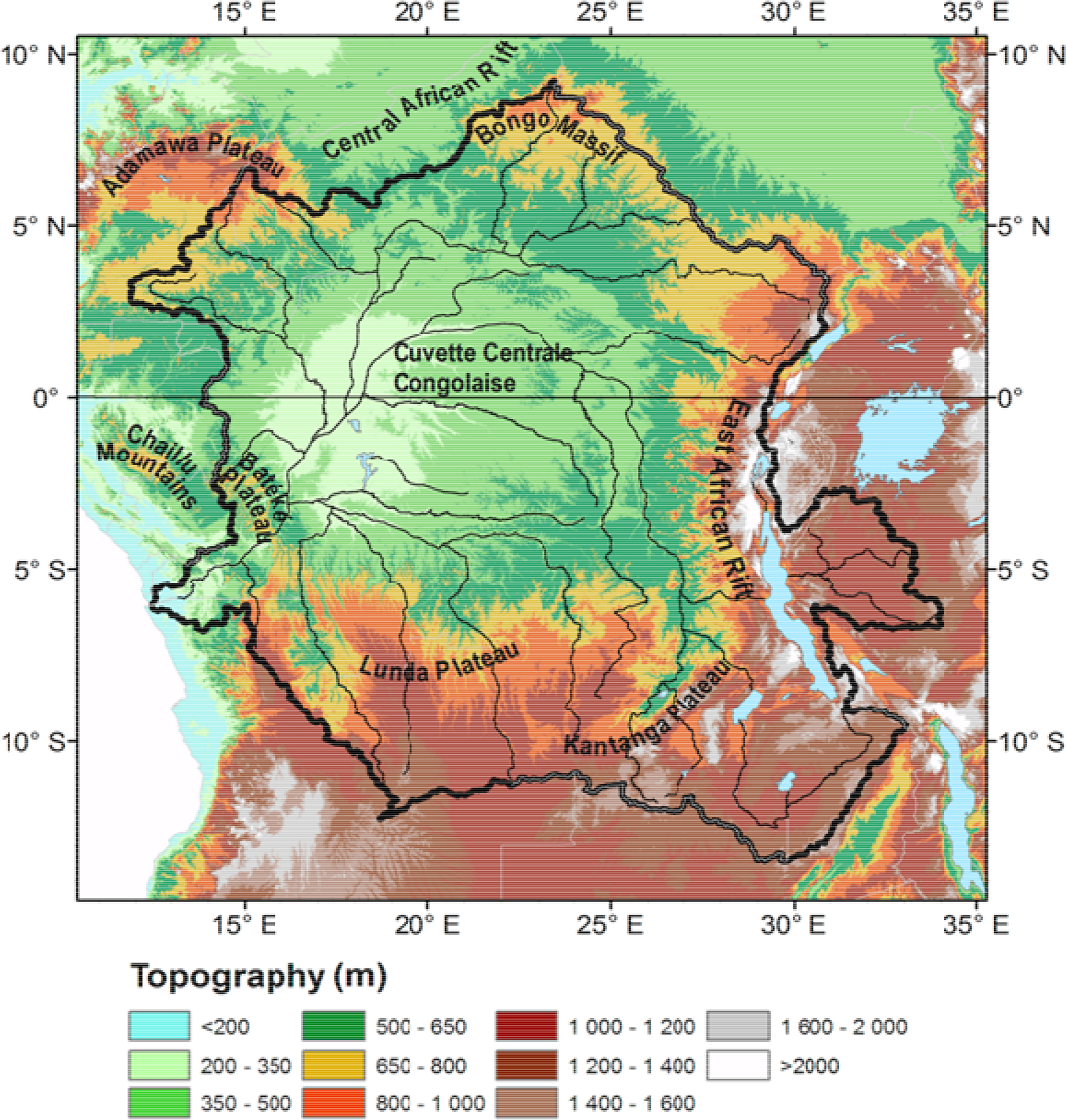
The Congo River Basin is a transboundary basin located in western equatorial Africa that extends over 3.7 million km2 (Figures 1 and 2). This shallow depression along the equator in the heart of Africa, named “Cuvette Central Caongolaise” [16], is bordered by higher areas (Figure 1): the Chaillu Mountains (900 m) and the Batéké Plateau (600–800 m) lie to the west and southwest.
North of the basin are the Adamawa Plateau (1500 m) and the flanks of the Central African Rift (600–700 m), the boundary between the Congo and the Chad Basins, and the Bongo Massif (1300 m and higher). To the east, the most important relief is that of the volcanic foothills of the East African Rift, which reach altitudes of 2000–3000 m. The Katanga and Lunda Plateaus (1000–1500 m) bound the southern part of this vast watershed.
2.2. Hydrological System
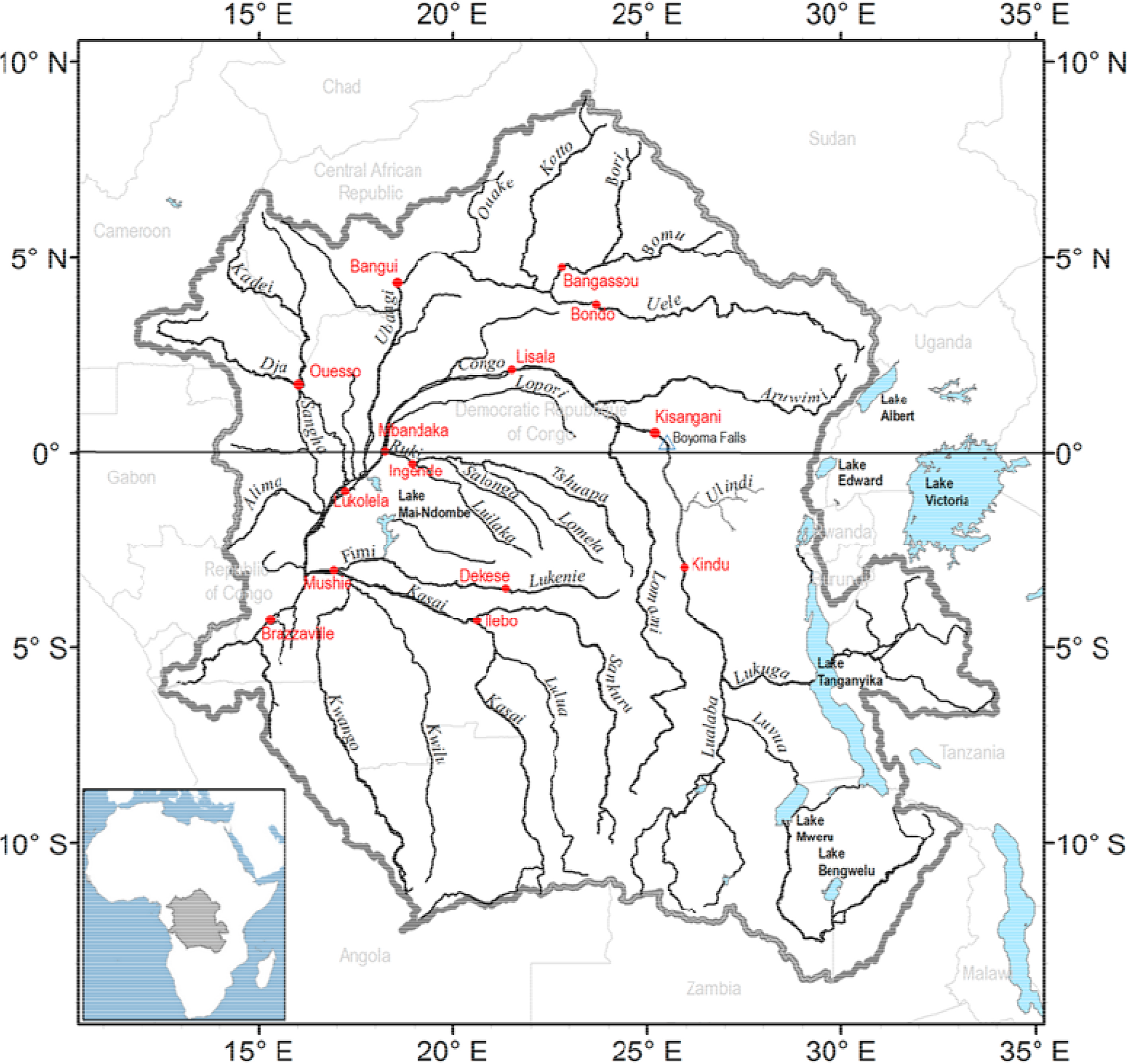
The Congo Basin features a complex hydrological system composed of the Congo River, its many tributaries, and extensive swamps. The sources of the Congo River are on the highlands of the East African Rift in Lake Tanganyika, which feeds the Lukuga and Lualaba Rivers; these become the Congo River at Kisangani, below Boyoma Falls (Figure 2). The other two principal tributaries of the Congo are the Kasai River from the south and the Ubangi River from the north.
The Ubangi River is formed by the confluence of the Uele and Bomu rivers. Other main tributaries of the Ubangi River are the Bori River, the Kotto River and the Ouake River. The major tributaries of the Kasai River are the Kwango River and the Lulua River. They join to form the Kasai River from the south and drain a large part of the southern and southwestern Democratic Republic of Congo and northern Angola. The Fimi/Lukenie system runs parallel to and just north of the main Kasai River. Water draining from Lake Mai-Ndombe empties south through the Fimi River into the Kasai River. The Sangha River is a second-order tributary of the Congo River.
2.3. Climate
The Congo River receives year-round rainfall from the migration of the Inter-Tropical Convergence Zone (ITCZ). The northern part of the basin experiences a minor rainy season from September to November and a major one from the first half of March to early May; in the south, the minor rainy season lasts from February to May, and the major rainy season occurs between September and December. The source regions receive an average annual rainfall of 1200 mm. The middle and the downstream parts of the watershed receive 1800–2500 mm of rainfall per year and experience almost no dry season [16–18].
3. Primary Datasets and Methods
3.1. Altimetry and Virtual Station Data
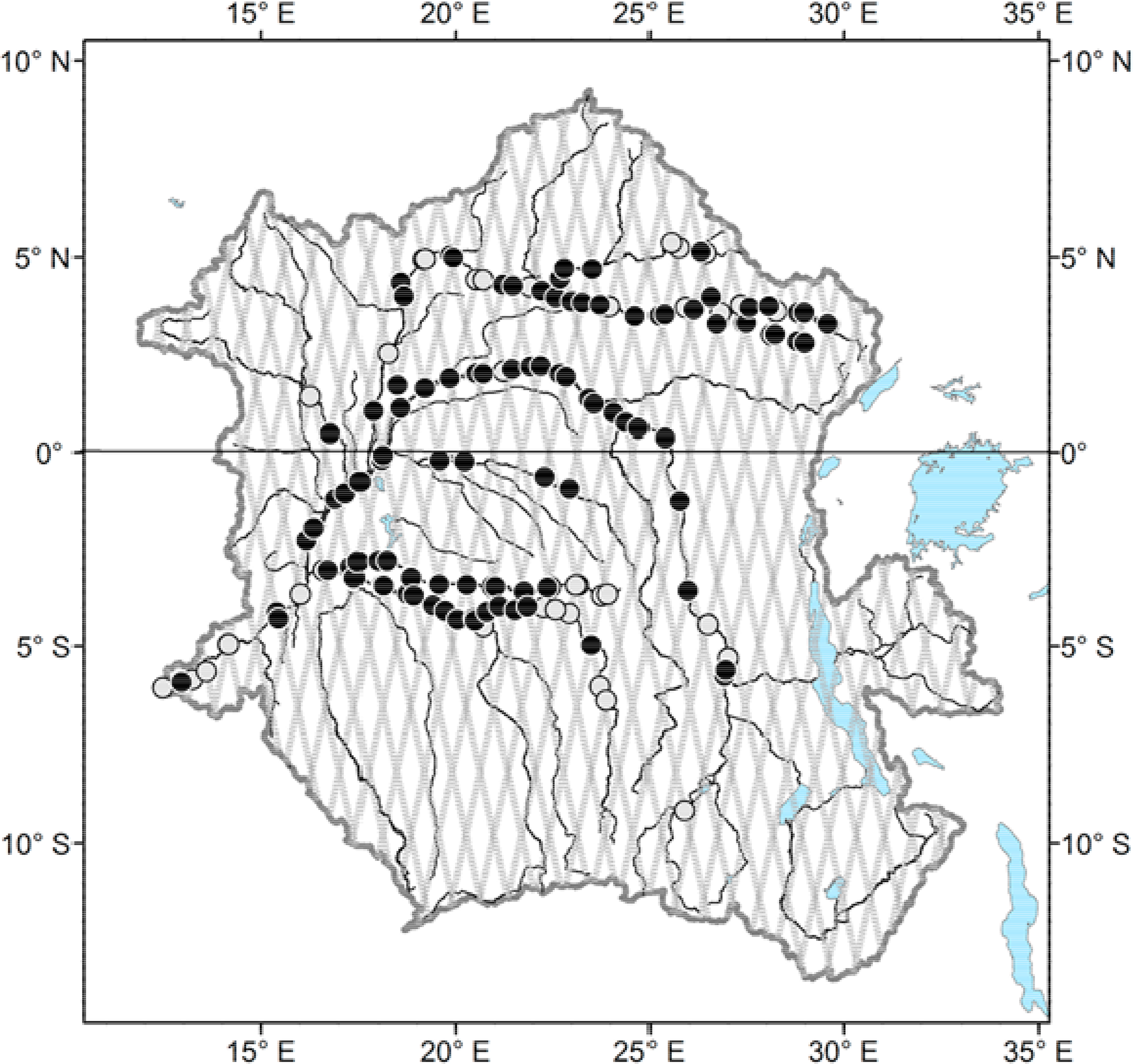
The European Space Agency launched the ENVIronmental SATellite (ENVISAT) in March 2002 as part of its Earth Observation Program. This mission concluded in April 2012. ENVISAT carried ten instruments [19], including a nadir radar altimeter (RA-2 or Advanced Radar Altimeter). The ground track of the nominal ENVISAT orbit over the Congo Basin is shown in Figure 3. At all points where a satellite track intersects a water body, or “virtual stations”, we extracted a water level time series, which allowed us to measure the successive water levels at each pass of the satellite over the large rivers channels, smaller tributaries and wetlands within sub-basins of the Congo Basin. The raw ENVISAT data are freely distributed by the Center for Topographic studies of the Ocean and Hydrosphere (CTOH, [20]) in the standardized format of along-track Geophysical Data Records (GDRs). These data include four estimates of the distance between the satellite antenna and the ground, or the range. These four ranges are obtained by processing the radar echo with a dedicated algorithm called a retracker. Although none of the four retrackers had been tuned for echoes from river surfaces, Frappart et al. [21] and Santos da Silva et al. [22] showed that the ice-1 algorithm [23] performed well over rivers. Therefore, in this study, we used the ice-1 ranges when processing the raw ENVISAT data to compute water level time series at each virtual station. Our corrections are of two types: propagation corrections and geophysical corrections. The geophysical corrections are designed to remove instantaneous crustal movements. We applied corrections for solid earth and polar tides. Propagation corrections are designed to correct for the propagation of the electromagnetic wave as the radar travels through an ionized medium, the ionosphere, and a dense medium, the troposphere. We applied the corrections derived from global models as provided in the GDRs, in particular the tropospheric corrections derived from the European Centre for Medium-Range Weather Forecasts (ECMWF) meteorological model. We obtained the water stage time series between 2003 and 2009 (complete years) at 140 virtual stations (Figure 3) using the Virtual ALtimetry Station Tool (VALS) [24] for the ENVISAT tracks crossing the Congo Basin.
Details regarding the procedure used to process the data using VALS can be found in Santos da Silva et al. [22]. In this study, the water level data are referenced to the EGM2008 geoid model [25]. The water level time series at every virtual station passed a quality control test for gaps and/or shifts in the data. All time series with gaps greater than 3 consecutive months were deleted. All time series with a visually detectable spurious strong shift were also deleted. For the remaining time series, outliers were identified using Rosner’s test [26] and removed. When small gaps (≤3 consecutive months) were observed, we reintroduced missing data by linearly interpolating the time series. Only 99 time series from the initial dataset of the 140 river water level series (RWL) satisfied these requirements (Figure 3). In this study, we use water level data rather than river discharge data. Because direct measurements of discharge in river channels can be time-consuming and costly, flow is often estimated indirectly by the rating curve method [27]. According to this technique, measurements of a river stage are converted to river discharge by a function (rating curve), which is preliminarily estimated by using a set of stage and flow measurements. Hence, uncertainties in measurements and the rating curve method increase the final uncertainty. Using the river level data is thus more straightforward in this region because we lack the data needed to calculate the rating curve at each virtual station. Moreover, this study uses water levels rather than discharge because, unlike in situ data, altimetry-derived stages are related to a common geoidal reference; the classification process used and described hereafter allows us to separate and analyze the section morphology effect while also not increasing the corresponding uncertainties by estimating discharge from stages.
3.2. Brazzaville Gauging Station
The time series of monthly water levels at Brazzaville (Figure 2. 15.3°E and 4.3°S) over the period 2003–2009 is selected from the Environmental Research Observatory HYBAM [28] Station: 50800000 Rio Congo at Congo Beach Brazzaville, covering the period from 1990 to the latest available year). This time series is used to evaluate our classification method. The same quality control process applied to the virtual stations was applied to this time series.
3.3. Lake Water Level
The monthly water level time series of Lake Mweru (Figure 2, 29.8°E and 8.7°S) and Lake Tanganyika (Figure 2, 29.5°E and 6.5°S) are available through Hydroweb [29]. Hydroweb is developed by LEGOS (Laboratoire d'Etudes en Géophysique Océanographie Spatiales) in France and provides water level time series of large rivers, approximately 150 lakes and reservoirs, and wetlands around the world using the merged data from the Topex/Poseidon, Jason-1, Jason-2, ENVISAT, European remote sensing satellite (ERS) and Geosat Follow-On (GFO) satellite missions. The processing procedures of Hydroweb are described in Crétaux et al. [30]. The Hydroweb lake water levels are monthly values obtained by merging measurements from different tracks of different altimeter satellites overflying the same lake in the same month [30]. These time series will be used to evaluate our classification method.
3.4. K-Means Clustering
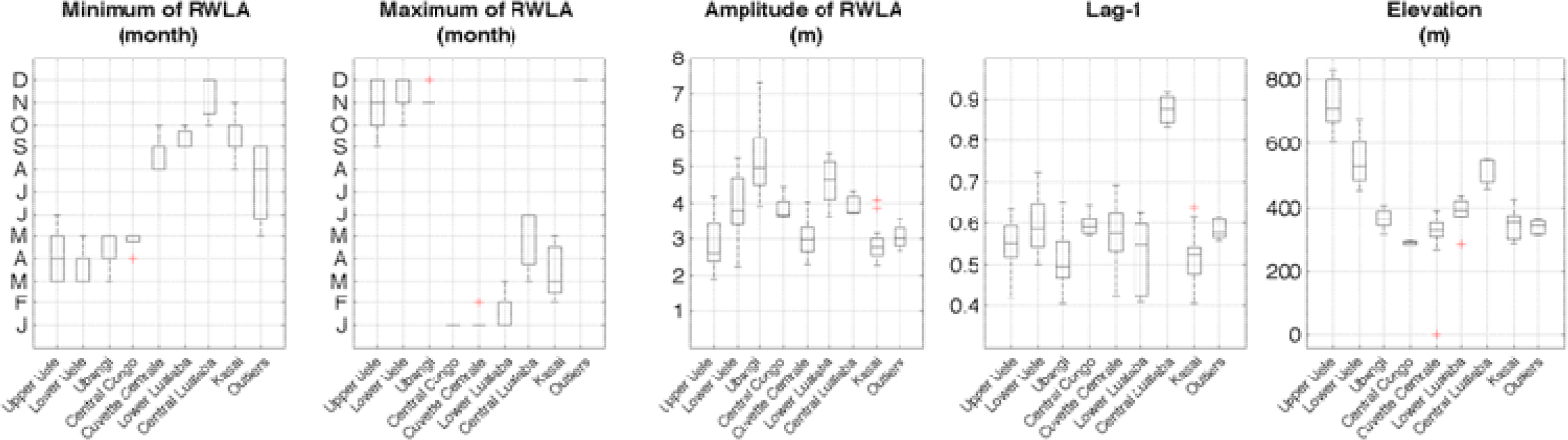
The K-means is a common algorithm for classifying objects into K clusters, with K being a positive integer number. The classification is performed by minimizing the sum of squares of distances between data and the corresponding cluster centroid. Thus, the sample is assigned to a cluster based on minimizing, in its simplest form, the Euclidean distance between the vector of its variables and the means of the variables within a cluster. The K-means algorithm proceeds by updating the mean and grouping the data again. This procedure continues until all samples no longer change clusters. Given a dataset, a desired number of clusters K, and a set of K initial starting points, the K-means clustering algorithm finds the desired number of distinct clusters and their centroids. The K-means algorithm is described in more detail by Hartigan [31] and Hartigan and Wong [32]. In hydrology, the K-means algorithm and its variants have been used primarily in the regionalization of watersheds [33–37]. In this study, K-means analysis is performed for predefined cluster numbers varying from 5 to 15, where 15 is the maximum number of groups that maintains sufficient sample sizes in each group. To choose the initial cluster centroid positions, we select K uniform points at random from the range of the normalized parameters. The chosen parameter vectors are elevation data based on the HydroSHEDS DEM data at 30 arc-second resolution [38], river water level anomaly (RWLA) amplitude, dates of low and high stages and interannual correlation structure (lag-1), representing the dynamic component of the process. For example, if the autocorrelation in a time series at lag-1 is high (>0.6) the values are highly correlated with the value in the previous month. We run 10,000 replicates from randomly chosen starting parameter vectors; all runs converge to the same solution. The optimal number of clusters to retain is determined with the aid of the Davies–Bouldin index, a cluster validity measure that is a function of the ratio of the sum of within-cluster dispersion to between-cluster separation [39]. We calculate the separation measure for numbers of clusters ranging from 5 to 15. We filter our results according to certain specific criteria, such as a homogeneous distribution of observations within each cluster and no single-member clusters.
4. Results of the RWLA K-Means Clustering
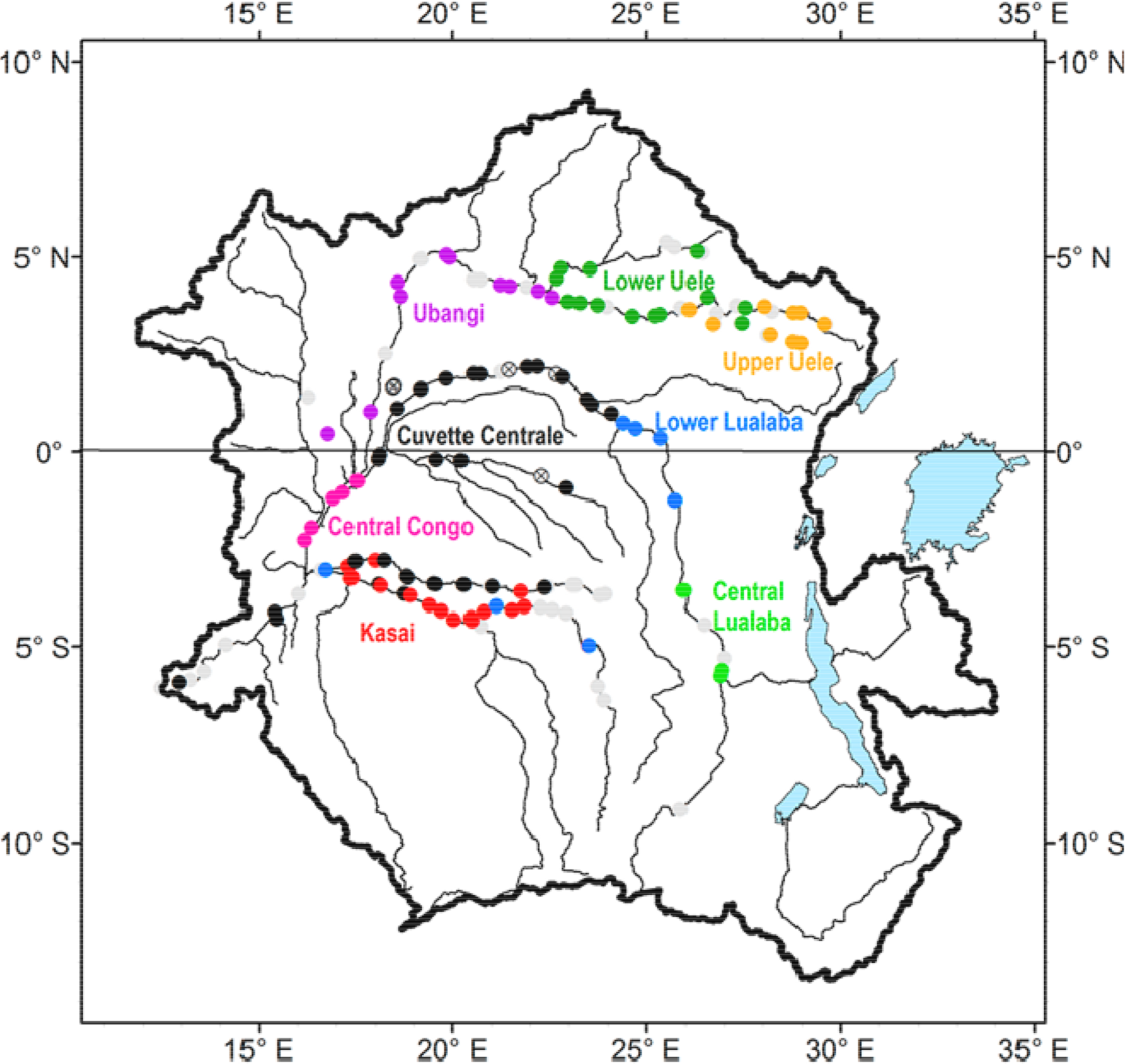
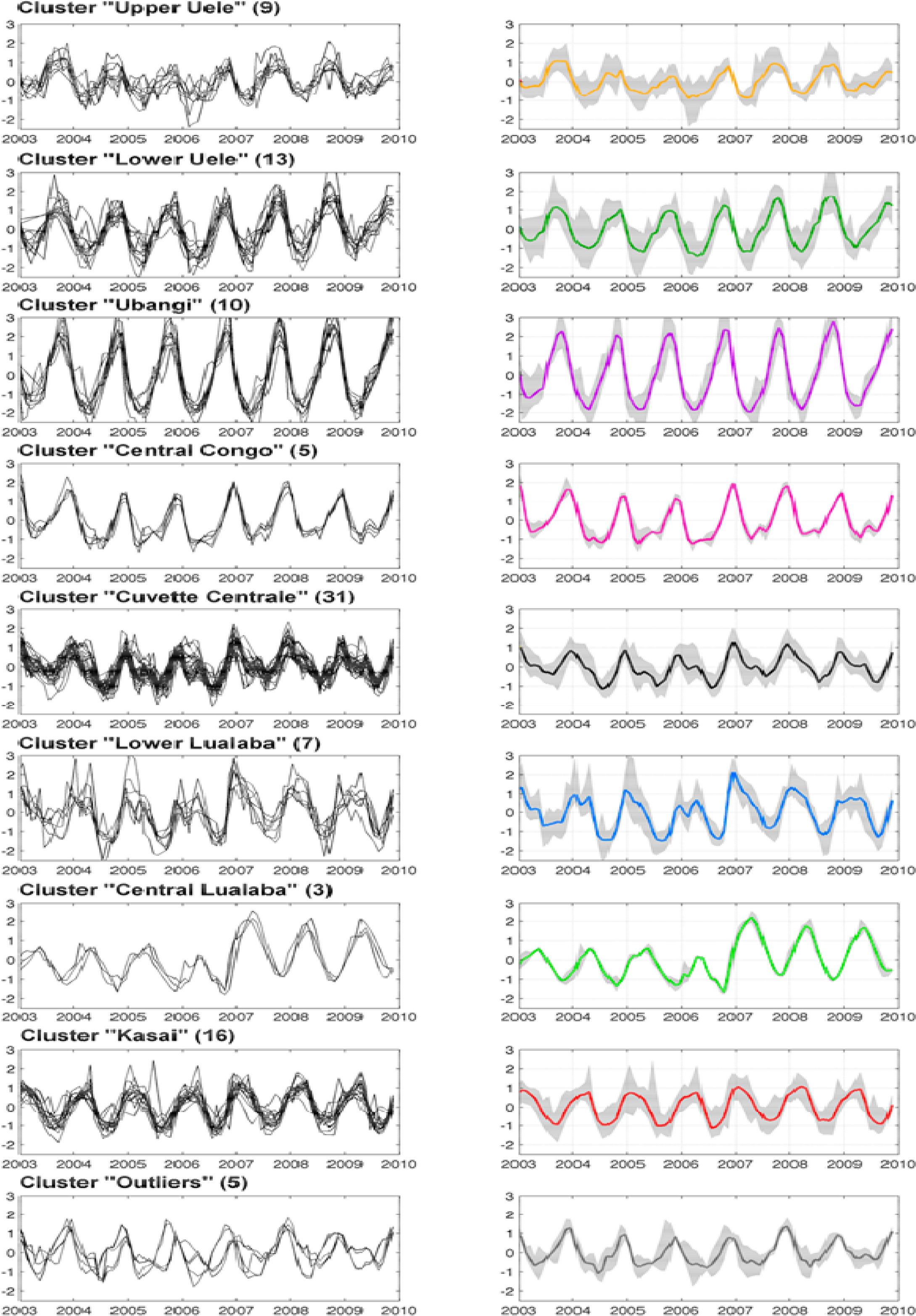
The first step of the proposed approach is to cluster the 99 time series of altimeter-derived RWLA to identify groups with similar characteristics, defined by a conservative set of morphometric and hydrologic parameters. This study is developed for the RWLA is hereafter defined as the difference between the water level value and the temporal mean of the time series. Finally, according to these requirements presented in Section 3.4, the RWLA dataset is divided into 9 clusters exhibiting similar features. The optimal cluster locations are shown in Figure 4, and a topology map of RWLA signature vectors is shown in Figure 5. The topology highlights the variation of the RWLA features along the different classes, characterizing the behavior of the input variables and their interrelations. The RWLA time series composing each cluster are shown in Figure 6.
Cluster “Upper Uele”, in the extreme northeast of the Congo Basin, contains 9 RWLA time series. Cluster “Lower Uele” contains the downstream part of the Uele River and its confluence with the Bomu River; the cluster includes 13 RWLA time series. Cluster “Ubangi” is composed of 10 RWLA time series. Cluster “Central Congo” contains 5 time series located along the Congo River after its confluence with the Ubangi River and prior to its confluence with the Kasai River. Cluster “Central Lualaba” includes 3 RWLA time series. Cluster “Lower Lualaba” is formed by 7 RWLA time series, 4 of which are located in the eastern part of the basin along the Lualaba River between the confluences with the Ulindi River and the Lomami River. The remaining 3 times series of this cluster are located along the Kasai River. For this cluster, we observe a large dispersion of the lag-1 coefficient, most likely because the RWLA time series are not located on the same rivers and therefore have different temporal correlation structures. Cluster “Cuvette Centrale” contains 31 RWLA time series. This cluster includes RWLA time series located in three regions: on the main stream of the Congo River between the confluences of the Lomami River and the Ubangi River, along the Ruki and Tshuapa Rivers, and along the Fimi and Lukenie Rivers. The 16 RWLA time series that compose Cluster “Kasai” are located in the meridional part of the Congo Basin. Cluster “Outliers” contains 4 RWLA time series spread throughout the basin. From the comparison shown in Figure 6, we can conclude that there is no good consistency between the time series in this cluster and we therefore removed it from consideration in the remainder of the study.
5. Validation of the RWLA Regionalization
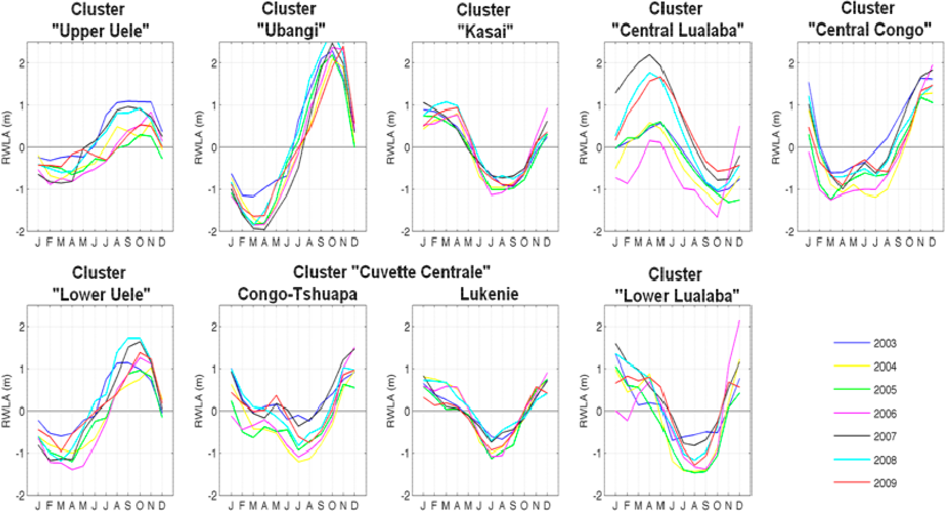
Mahé [40] defined four great climatic zones over the Congo Basin: the North (Ubangi River Basin), where the influence of the North African continental air mass is prominent; the South (Kasai River Basin), which is influenced by South African air masses; the eastern and south-eastern parts of the basin (Lualaba River Upper Basin), which are influenced by the humid Indian Ocean air masses; and the Center-West, where the climate is controlled by the Atlantic Ocean. The seasonal partition of rainfall is bimodal along the equator and becomes unimodal farther north and south. We should therefore typically observe two-peak hydrographs (bimodal) for rivers near the equator and a gradual transformation into one-peak hydrographs (unimodal) farther north and south of the equator. We use this hypothesis to validate our RWLA regionalization. Figure 7 shows the hydrographs of monthly mean RWLA from 2003 to 2009 for each cluster. For each of the clusters, we verify that their time series show the same seasonal dynamics.
5.1. The North-Ubangi River Basin
Cluster “Upper Uele”: We observe a unimodal distribution of the RWLA in all years except 2009. This cluster is characterized by a high water level from September to November and a low water level from February to March. The transition period, May to June, is very short. The years 2004, 2005, 2006 and 2009 were particularly dry (average RWLA < 0.5 m), whereas in 2003, the RWLA was greater than 1 m for 4 months (August through November). The seasonal variability contributed between 1 to 1.8 m over this period.
Cluster “Lower Uele”: The distribution of RWLA is unimodal, with low water levels from March to April and high water levels from September to October. These dynamics are comparable to the monthly maxima and minima recorded by the historical river gauge at Bondo in 1956, located on the Uele River (Rosenqvist and Birkett [10], in Table 2). The seasonal amplitude is approximately 3 m over our study period.
Cluster “Ubangi”: The RWLA time series of this cluster are relatively homogeneous from 2003 to 2009. The distribution is unimodal. The dry season occurs from December through March (4 months), followed by rising water in May and a high water level in October. From November to January (3 months), we observe a rapid decrease in water level. These dynamics are similar to the monthly maxima and minima recorded by the historical river gauge at Bangui over 1890–1955, located on the Ubangi River ([10], in Table 2). This cluster has the largest seasonal variability in terms of RWLA, approximately 4.1 m over our study period.
5.2. The Southeast–Central and Upper Basins of the Lualaba River
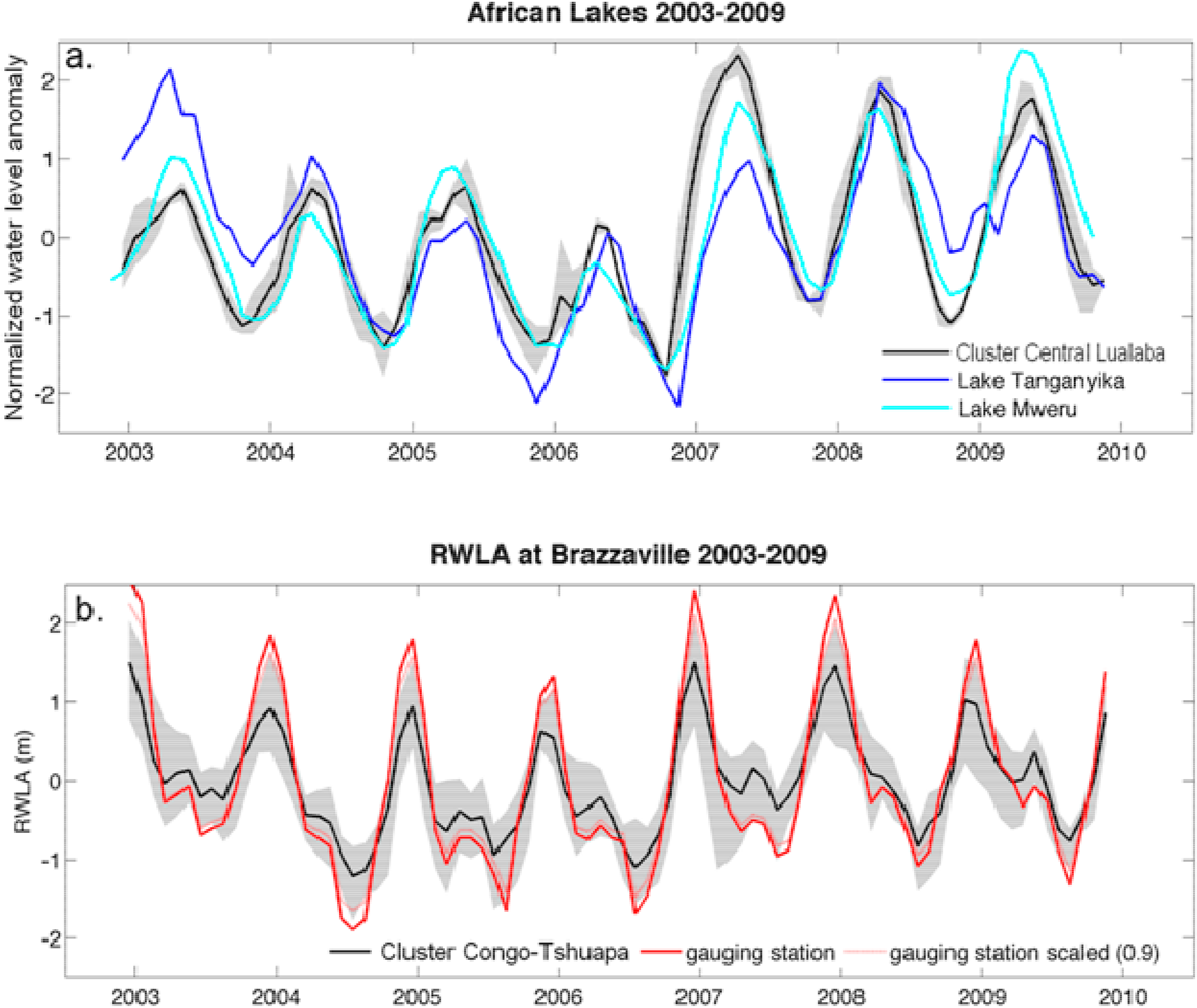
Cluster “Central Lualaba”: The RWLA in this cluster shows marked variability from one year to another. The distribution of the RWLA is unimodal, with high water levels from April to May and low water levels in October. These dynamics are consistent with the changes in water level recorded by the historical river gauge at Kindu over 1912–1955, located on the Lualaba River (Table 2 in Rosenqvist and Birkett 2002 [10]). We can observe 2 different periods in RWLA: (1) the seasonal variability from 2003 to 2006 shows well-marked minima and maxima but slight amplitude variations; (2) the seasonal variability over 2007–2009 shows well-marked minima and maxima and very large amplitude variations. In 2007, the extreme anomaly (2.2 m) was, on average, 4 times greater than the minimum values during the first period (∼0.5 m). We observe evidence of completely different behavior of the RWLA in the year 2006. The temporal structure of low and high water levels is retained, but all the values are either near 0 m or negative, except in December. During the 3 months from October to December, we observe an increase in water level by more than 2.2 m. This extreme RWLA variability in 2006 and 2007 can be explained by hydro-climatic changes occurring in the East African Rift region. This cluster is located downstream on the Lualaba River (elevation ∼500 m), which is fed by Lake Tanganyika and Lake Mweru. The extreme water levels are most likely related to the 2005 severe drought reported in Equatorial East Africa [41] and to the positive strong Indian Ocean Dipole (IOD) in 2006. Similar behavior has been noted for other continental water cycle parameters. For example, Becker et al. [42] confirmed that precipitation and terrestrial water storage in the East African great lakes region have a common mode of variability, with a minimum in late 2005 and a sharp rise in 2006–2007. The authors showed that this event was due to forcing by the 2006 IOD on East African rainfall. As expected, we observe asymmetry in RWLA seasonal variability between the northern and the southern regions due to their locations on both sides of the equator. A comparison between the RWLA mean time series from the “Central Lualaba” cluster and the water level (WL) time series of Lake Mweru and Lake Tanganyika, computed from the T/P, Jason-1, Jason-2, ENVISAT, ERS and GFO satellite missions and provided by Hydroweb is presented in Figure 8a. The Luvua River exits Lake Mweru and flows northwest, and the Lukuga River drains Lake Tanganyika. These 2 rivers join the cluster on the Lualaba River.
The RWLA seasonal variability from the cluster agrees well with the WL seasonal variability of the two lakes. We observe a lagged correlation coefficient of 0.9 between the cluster RWLA and Lake Mweru WL with a delay of 1–2 months for the Lake Mweru WL. Further work concerning the hydrology of this region is necessary to explain the 1–2 month delay observed between the cluster and Lake Mweru. The correlation coefficient is 0.7 (p-value < 0.001) between the RWLA cluster and the Lake Tanganyika WL; no significant delay is detected between these two curves. A slight trend is observed in the Lake Tanganyika WL before 2007, but it is not observed in the RWLA of the cluster and Lake Mweru. Such consistency between the RWLA and WL time series enables us to validate this cluster.
5.3. The South-Kasai River Basin
Cluster “Kasai”: We observe a unimodal RWLA distribution of this cluster time series over the studied period. The RWLA minima occur from August to September, and the maxima occur from January to April. RWLA maxima occur in January (2003, 2005 and 2007) or April (2004, 2006, 2008 and 2009), usually in alternating years. The seasonal variability is between 1.8 and 2 m over the period. These dynamics are comparable with the monthly maxima and minima distribution recorded by the historical river gauge at Mushie in 1932–1955 and at Ilebo in 1924–1955, both located on the Kasai River ([10], in Table 2).
5.4. The Center-West–Congo River Basin
Cluster “Cuvette Centrale”: This cluster holds the largest number of RWLA time series (31) and has the largest latitudinal variability (from 2.5°N to 6°S). To avoid over-parameterization, we do not include prior information regarding the latitude coordinate or the RWLA bimodal/unimodal seasonal signature in the K-means clustering method. It is thus prudent to check the homogeneity of the RWLA seasonal variability within this cluster. As might be expected, we clearly observe 2 sub-clusters: (1) 20 RWLA time series located on the main stream of the Congo River and the Tshuapa River (hereafter named Cluster “Congo-Tshuapa”); (2) 11 RWLA time series located on the Lukenie River (hereafter named Cluster “Lukenie”). The RWLA time series of the cluster “Congo-Tshuapa” has a bimodal distribution. The water levels begin to rise in August and September due to rainfall intensification in the southern hemisphere. The high-water period is reached in December and lasts a relatively short time. The secondary low-water period occurs in March, during the dry season that prevails in the northern hemisphere tributaries. The primary low-water period in July and August corresponds to the dry season that prevails in the southern hemisphere [43]. These results are validated by the dynamics of the historical river gauge records at Mbandaka over 1913–1955 and at Lisala over 1914–1955, both located on the Congo River, and at Ingende over 1933–1955, located on the Ruki River ([10], in Table 2). We notice a contrast between the very dry years 2004, 2005 and 2006, when low water levels lasted 8, 9 and 10 months, respectively, and the years 2003, 2007, 2008 and 2009, when the low-water periods were almost non-existent. The average seasonal variability over our study period is on average 1.8 m, except in 2006 when it was 2.6 m, twice the amplitude observed in 2003.
Figure 8b shows a comparison between the RWLA time series from the cluster “Congo-Tshuapa” and the RWLA time series recorded at the Brazzaville gauging station over the period 2003–2009. These two RWLA time series are remarkably synchronized and have a correlation coefficient of 0.96 (p-value < 0.001). However, the RWLA time series recorded at Brazzaville shows an amplitude 10% greater than the 95% confidence upper and lower bounds. Although not shown in the figure, the Brazzaville gauge also has a significant correlation coefficient (p-value < 0.001) with respect to the RWLA of Cluster “Central Congo” (0.9), Cluster “Lower Lualaba” (0.75), Cluster “Lukenie” (0.75) and Cluster “Kasai” (0.5).
The RWLA time series of Cluster “Lukenie” has unimodal dynamics and is relatively homogeneous from 2003 to 2007. The dates of extreme water levels coincide with those of the Cluster “Congo-Tshuapa”: minimum in July and maximum in December and January. The seasonal variability over our study period averages 1.8 m. These results are similar to the historical water level time series records at Dekese over 1932–1955, located on the Lukenie River ([10], in Table 2).
Cluster “Central Congo”: The RWLA stations are located on the Congo River downstream of its confluence with the Ubangi River and before its confluence with the Kasai River. This cluster is located in a hydrographically complex region and is influenced by three major rivers: the Ubangi, the Upper Congo and the Sangha [44]. The bimodal water level dynamics are very similar to those of Cluster “Congo-Tshuapa”: high water levels from November to December and a second high-water period from May to June. However, in Cluster “Central Congo”, low water levels occur in March and another more extreme low occurs in July, which is nearly the opposite of the Cluster “Congo-Tshuapa” dynamics. This finding can be explained by the strong influence of the Ubangi River (Cluster “Ubangi”), which is positive in the wet season (September) and negative in the dry season (March). Moreover, the RWLA seasonal variability is consistent with the dynamics at the Ouesso historical river gauge on the Sangha River (from the Global Runoff Data Center, [45]) and with the monthly maxima and minima recorded by the historical river gauge at Lukolela over 1909–1955, located on the Congo River ([10], in Table 2). The low-water period is very long, lasting 7 to 8 months. The seasonal variability is, on average, 2.4 m over our study period, except in 2006, when it was 3.2 m.
Cluster “Lower Lualaba”: We apply the same methodology as that applied to Cluster “Cuvette Centrale” to the 7 time series that make up this cluster, but we do not observe any significant difference in seasonal variability between the RWLA time series from the Kasai River and the RWLA time series located on the lower Lualaba River. The RWLA hydrograph for Cluster 8 has a unimodal distribution, except for the years 2004 and 2006, for which a second high-water period occurs in April. The maximum occurs in December-January and the minimum in August. These results are validated by the historical water level time series recorded at Kisangani from 1907–1955, located on the Upper Congo River ([10], in Table 2). We note that in this region, the RWLA seasonal variability is, on average, 2.5 m over our study period, except in 2006, when it was 3.5 m.
We investigate the regionalization that these clusters suggest. Clusters “Upper Uele”, “Lower Uele” and “Ubangi” spatially match the northern region as described by Mahé [36]. The increasing amplitude from upstream to downstream is coherent with the gathering of water along the river system. Cluster “Central Lualaba” represents the eastern and southeastern parts of the basin and is very distinct from the other clusters. The southern and central western regions are not very well represented by the clusters considered in the present study. Cluster “Lower Lualaba” appears intermediate between Cluster “Central Lualaba” and all other clusters. Clusters “Central Congo” and “Congo-Tshuapa” are bimodal, similar to each other, and separated from Clusters “Kasai” and “Lukenie”. Our data suggest that regionalization in the central part of the catchment follows more of an east-west gradient than a north-south one.
6. Further Research
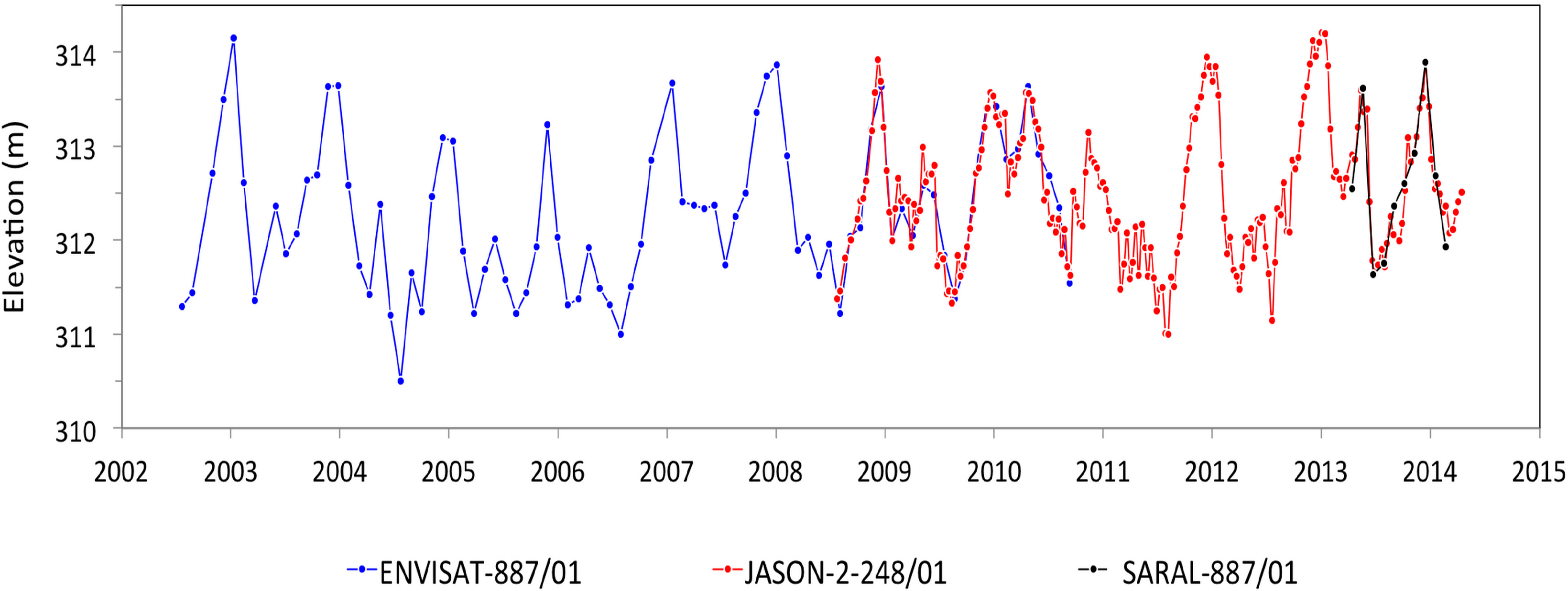
The dataset used in the present study is currently being expanded. In terms of spatial extent, many other virtual stations are currently being computed from ENVISAT to sample more rivers, such as the Kwango and Kwilu Rivers in the southwestern part of the basin, the Dja River in the northwestern part of the basin and in the east, and the Lukuga and Luvua Rivers, which drain the Tanganika and Mweru Lakes, respectively, into the Congo River. In terms of temporal extent, the 7-year ENVISAT time series will soon be extended with data from new satellites: Jason-2, launched in June 2008, and SARAL, launched in February 2013. Combining Jason-2 and SARAL observations for land water monitoring will take advantage of the 10-day temporal resolution of Jason-2 and the high geographical coverage of SARAL, which flies along the same orbit as ENVISAT. An example of a long series over the Congo River that can be obtained by combining ENVISAT, Jason-2 and SARAL data is shown in Figure 9.
7. Conclusion
This study was conducted using stage rather than discharge measurements, which makes it unusual within the field of hydrology. The utility of altimeter-derived information is illustrated by finding the spatial and temporal signatures of climate variability in water level variations within the Congo Basin. Studies of this type have been traditionally based on historical in situ gauging station records, when and where available. However, climate and hydrological networks are sparse within the Congo Basin. Using satellite altimetry, we constructed a very large number of virtual stations across the Congo Basin to obtain information on the regional variability of surface water level anomalies in places where no in situ data are available over the period 2003–2009. This study shows that water levels can be measured throughout the basin, even in remote places, including the upstream, narrow parts of rivers. The study yielded interesting insights into the regionalization and characterization of the hydrological regime of the Congo Basin. Our analyses show an east-west gradient that has not previously been identified. The central western region is limited to a small region near the Congo swamp and represents the only bimodal hydrological regime of the basin. The Kasai region is similar to the central eastern region and is a progressive transition zone with the southeastern region. In conclusion, we have been validated the proposed regionalization scheme. Therefore considered reliable for estimating monthly water level variations in the Congo Basin. This result confirms the potential of satellite altimetry in monitoring spatio-temporal water level variations as a promising and unprecedented means for improved representation of the hydrologic characteristics in large ungauged river basins.
Acknowledgments
We thank the CTOH for providing the ENVISAT GDR data. M. Becker is supported by the Centre National d’Etudes Spatiales (CNES) and a Fonds social européen (FSE) fellowship. This study was supported by the AforA project within the CNES/TOSCA fund. We thank the three anonymous reviewers for their careful reading of our manuscript and their many insightful comments and suggestions.
Authors’ Contributions
Mélanie Becker conducted the data analysis and wrote the majority of the paper. Joecila Santos da Silva was responsible for the processing of the ENVISAT observations. Stéphane Calmant supervised the research and contributed to manuscript organization and writing. Vivien Robinet contributed to the design of the regionalization method. Laurent Linguet and Frédérique Seyler helped with discussions and manuscript revisions.
Conflicts of Interest
The authors declare no conflict of interest.
References
- Devroey, E. Observations Hydrographiques du Bassin Congolais (1932–1947). Available online: http://www.worldcat.org/title/observations-hydrographiques-du-bassin-congolais-1932-1947/oclc/8209249 (accessed on 16 May 2014).
- Charlier, J. Études Hydrographiques Dans Le Bassin Du Lualaba, Congo Belge, 1952–1954; Comité Hydrographique du Bassin Congolais: Bruxelles, Belgium, 1955. [Google Scholar]
- Snel, M.J. Contribution à l’étude Hydrogéologique du Congo Belge. Service Géologique, Bulletin No. 7; Democratic Republic of the Congo: Kinshasa, Democratic Republic of the Congo, 1957; Volume 2. [Google Scholar]
- Hochschild, A. King Leopold’s Ghost: A Story of Greed, Terror and Heroism in Colonial Africa; Houghton Mifflin: Boston, MA, USA, 1998. [Google Scholar]
- Ndaywel è Nziem, I.; Obenga, T.; Salmon, P. Histoire du Zaïre: De L’héritage ancien à L’âge Contemporain; Duculot: Louvain-la-Neuve, Belgique, 1997. [Google Scholar]
- Campbell, D. The Congo River basin. In The World largest Wetlands: Ecology and Conservation; Cambridge University Press: Cambridge, UK, 2005; pp. 149–165. [Google Scholar]
- Shem, O.W.; Dickinson, R.E. How the Congo basin deforestation and the equatorial monsoonal circulation influences the regional hydrological cycle. Proceedings of the 86th Annual American Meteorological Society Meeting, Atlanta, GA, USA, Tuesday, 31 January 2006; 2006. [Google Scholar]
- Alsdorf, D.E.; Rodrfgue, E.; Lettenmaier, D. Measuring Surface Water from Space. Available online: http://bprc.osu.edu/hydro/publications/2007a_Alsdorf.pdf (accessed on 16 May 2014).
- Tang, Q.; Gao, H.; Lu, H.; Lettenmaier, D.P. Remote sensing: Hydrology. Prog. Phys. Geogr 2009, 33, 490–509. [Google Scholar]
- Rosenqvist, A.A.; Birkett, C.M. Evaluation of JERS-1 SAR mosaics for hydrological applications in the Congo River Basin. Int. J. Remote Sens 2002, 23, 1283–1302. [Google Scholar]
- Eltahir, E.A.; Loux, B.; Yamana, T.K.; Bomblies, A. A see-saw oscillation between the Amazon and Congo basins. Geophys. Res. Lett 2004, 31. [Google Scholar] [CrossRef]
- Crowley, J.W.; Mitrovica, J.X.; Bailey, R.C.; Tamisiea, M.E.; Davis, J.L. Land water storage within the Congo Basin inferred from GRACE satellite gravity data. Geophys. Res. Lett 2006, 33. [Google Scholar] [CrossRef]
- Jung, H.C.; Hamski, J.; Durand, M.; Alsdorf, D.; Hossain, F.; Lee, H.; Hossain, A.K.M.; Hasan, K.; Khan, A.S.; Hoque, A.K.M. Characterization of complex fluvial systems using remote sensing of spatial and temporal water level variations in the Amazon, Congo, and Brahmaputra Rivers. Earth Surf. Process Landf 2010, 35, 294–304. [Google Scholar]
- Lee, H.; Beighley, R.E.; Alsdorf, D.; Jung, H.C.; Shum, C.K.; Duan, J.; Guo, J.; Yamazaki, D.; Andreadis, K. Characterization of terrestrial water dynamics in the Congo Basin using GRACE and satellite radar altimetry. Remote Sens. Environ 2011, 115, 3530–3538. [Google Scholar]
- O’Loughlin, F.; Trigg, M.A.; Schumann, G.-P.; Bates, P.D. Hydraulic characterization of the middle reach of the Congo River. Water Resour. Res 2013, 49, 5059–5070. [Google Scholar]
- Bernard, E. Le Climat Écologique: De la Cuvette Centrale Congolaise. Available online: http://www.persee.fr/web/revues/home/prescript/article/geo_0003-4010_1948_num_57_305_12165 (accessed on 16 May 2014).
- Bultot, F. Atlas Climatique du Bassin Congolais. Available online: http://lib.ugent.be/catalog/rug01:001906688?i=0&q=000000869163 (accessed on 16 May 2014).
- Mahe, G.; L’hote, Y.; Olivry, J.C.; Wotling, G. Trends and discontinuities in regional rainfall of West and Central Africa: 1951–1989. Hydrol. Sci. J 2001, 46, 211–226. [Google Scholar]
- Wehr, T.; Attema, E. Geophysical validation of ENVISAT data products. Adv. Space Res 2001, 28, 83–91. [Google Scholar]
- Center for Topographic studies of the Ocean and Hydrosphere (CTOH). Available online: http://ctoh.legos.obs-mip.fr/ (accessed on 16 September 2014).
- Frappart, F.; Calmant, S. Cauhopvalidation of ENVISAT data products and Central Africa: 1951s in the Congo Basin using GRACE and satellite radar altimetry. Remote Sens. Environ 2006, 100, 252–264. [Google Scholar]
- Santos da Silva, J.; Calmant, S.; Seyler, F.; Rotunno Filho, O.C.; Cochonneau, G.; Mansur, W.J. Water levels in the Amazon basin derived from the ERS 2 and ENVISAT radar altimetry missions. Remote Sens. Environ 2010, 114, 2160–2181. [Google Scholar]
- Bamber, J.L. Ice sheet altimeter processing scheme. Int. J. Remote Sens 1994, 15, 925–938. [Google Scholar]
- VALS Tool Virtual ALtimetry Station. VALS Version 0.5.7, 2009. Available online: http://www.ore-hybam.org/index.php/eng/Software/VALS (accessed on 16 May 2014).
- Pavlis, N.K.; Holmes, S.A.; Kenyon, S.C.; Factor, J.K. The development and evaluation of the Earth Gravitational Model 2008 (EGM2008). J. Geophys. Res. Solid Earth 2012, 117. [Google Scholar] [CrossRef]
- Rosner, B. On the detection of many outliers. Technometrics 1975, 17, 221–227. [Google Scholar]
- Clarke, R.T. Uncertainty in the estimation of mean annual flood due to rating-curve indefinition. J. Hydrol 1999, 222, 185–190. [Google Scholar]
- ORE HYBAM—The Environmental Research Observatory on the Rivers of the Amazon Basin. Available online: http://www.ore-hybam.org/ (accessed on 18 September 2014).
- Hydroweb—Hydrology from Space. Available online: http://www.legos.obs-mip.fr/fr/soa/hydrologie/hydroweb/Page_2.html (accessed on 18 September 2014).
- Crétaux, J.-F.; Jelinski, W.; Calmant, S.; Kouraev, A.; Vuglinski, V.; Bergé-Nguyen, M.; Gennero, M.-C.; Nino, F.; Abarca, Del; Rio, R.; Cazenave, A. SOLS: A lake database to monitor in the Near Real Time water level and storage variations from remote sensing data. Adv. Space Res 2011, 47, 1497–1507. [Google Scholar]
- Hartigan, J.A. Clustering Algorithms; Wiley: New York, NY, USA, 1975. [Google Scholar]
- Hartigan, J.A.; Wong, M.A. Algorithm AS 136: A k-means clustering algorithm. J. R. Stat. Soc. Ser. C Appl. Stat 1979, 28, 100–108. [Google Scholar]
- Bhaskar, N.R.; O’Connor, C.A. Comparison of method of residuals and cluster analysis for flood regionalization. J. Water Resour. Plan. Manag 1989, 115, 793–808. [Google Scholar]
- Burn, D.H.; Goel, N.K. The formation of groups for regional flood frequency analysis. Hydrol. Sci. J. 2000, 45, 97–112. [Google Scholar]
- Rao, A.R.; Srinivas, V.V. Regionalization of watersheds by hybrid-cluster analysis. J. Hydrol 2006, 318, 37–56. [Google Scholar]
- Isik, S.; Singh, V.P. Hydrologic regionalization of watersheds in Turkey. J. Hydrol. Eng 2008, 13, 824–834. [Google Scholar]
- Toth, E. Catchment classification based on characterisation of streamflow and precipitation time series. Hydrol. Earth Syst. Sci 2013, 17. [Google Scholar] [CrossRef]
- Hydrological Data and Maps Based on SHuttle Elevation Derivatives at Multiple Scales USGS HydroSHEDS. Available online: http://hydrosheds.cr.usgs.gov/index.php (accessed on 18 September 2014).
- Davies, D.L.; Bouldin, D.W. A cluster separation measure. IEEE Trans. Pattern Anal. Mach. Intell 1979, PAMI-1, 224–227. [Google Scholar]
- Mahé, G. Modulation annuelle et fluctuations interannuelles des précipitations sur le bassin versant du Congo. Grands bassins fluviaux périatlantiques, ORSTOM, Paris, France, 1995, 13–26. [Google Scholar]
- Hastenrath, S.; Polzin, D.; Mutai, C. Diagnosing the 2005 drought in equatorial East Africa. J. Clim 2007, 20. [Google Scholar] [CrossRef]
- Becker, M.; Llovel, W.; Cazenave, A.; Güntner, A.; Crétaux, J.-F. Recent hydrological behavior of the East African great lakes region inferred from GRACE, satellite altimetry and rainfall observations. Comptes Rendus Geosci 2010, 342, 223–233. [Google Scholar]
- Vennetier, P. Géographie du Congo-Brazzaville. Available online: http://horizon.documentation.ird.fr/exl-doc/pleins_textes/divers11-11/01471.pdf (accessed on 16 May 2014).
- Laraque, A.; Orange, D.; Maziezoula, B.; Olivry, J.-C. Origine des variations de debits du Congo à Brazzaville durant le XXème siècle. In Water Resources Variability in Africa during the 20th Century; Servat, E., Hughes, D., Fritsch, J.-M., Hulme, M., Eds.; AISH: Wallingford, UK, 1998; pp. 171–179. [Google Scholar]
- GRDC—Global Runoff Data Center, Zaire—Ouesso Station. Available online: http://www.grdc.sr.unh.edu/html/Polygons/P1448100.html (accessed on 18 September 2014).


© 2014 by the authors; licensee MDPI, Basel, Switzerland This article is an open access article distributed under the terms and conditions of the Creative Commons Attribution license (http://creativecommons.org/licenses/by/4.0/).
Share and Cite
Becker, M.; Da Silva, J.S.; Calmant, S.; Robinet, V.; Linguet, L.; Seyler, F. Water Level Fluctuations in the Congo Basin Derived from ENVISAT Satellite Altimetry. Remote Sens. 2014, 6, 9340-9358. https://doi.org/10.3390/rs6109340
Becker M, Da Silva JS, Calmant S, Robinet V, Linguet L, Seyler F. Water Level Fluctuations in the Congo Basin Derived from ENVISAT Satellite Altimetry. Remote Sensing. 2014; 6(10):9340-9358. https://doi.org/10.3390/rs6109340
Chicago/Turabian StyleBecker, Mélanie, Joecila Santos Da Silva, Stéphane Calmant, Vivien Robinet, Laurent Linguet, and Frédérique Seyler. 2014. "Water Level Fluctuations in the Congo Basin Derived from ENVISAT Satellite Altimetry" Remote Sensing 6, no. 10: 9340-9358. https://doi.org/10.3390/rs6109340