Transforming Image-Objects into Multiscale Fields: A GEOBIA Approach to Mitigate Urban Microclimatic Variability within H-Res Thermal Infrared Airborne Flight-Lines

 ,
, 
Abstract
: In an effort to minimize complex urban microclimatic variability within high-resolution (H-Res) airborne thermal infrared (TIR) flight-lines, we describe the Thermal Urban Road Normalization (TURN) algorithm, which is based on the idea of pseudo invariant features. By assuming a homogeneous road temperature within a TIR scene, we hypothesize that any variation observed in road temperature is the effect of local microclimatic variability. To model microclimatic variability, we define a road-object class (Road), compute the within-Road temperature variability, sample it at different spatial intervals (i.e., 10, 20, 50, and 100 m) then interpolate samples over each flight-line to create an object-weighted variable temperature field (a TURN-surface). The optimal TURN-surface is then subtracted from the original TIR image, essentially creating a microclimate-free scene. Results at different sampling intervals are assessed based on their: (i) ability to visually and statistically reduce overall scene variability and (ii) computation speed. TURN is evaluated on three non-adjacent TABI-1800 flight-lines (∼182 km2) that were acquired in 2012 at night over The City of Calgary, Alberta, Canada. TURN also meets a recent GEOBIA (Geospatial Object Based Image Analysis) challenge by incorporating existing GIS vector objects within the GEOBIA workflow, rather than relying exclusively on segmentation methods.1. Introduction
Thermal infrared (TIR) remote sensing entails the acquisition, processing and analysis of remote sensing data acquired in the thermal infrared region (3–14 µm) of electromagnetic spectrum [1]. Currently, non-military TIR satellite sensors have moderate to low spatial resolution capabilities (e.g., 90 m ASTER, to 1.0 km NOAA-AVHRR). Consequently, studies using these data are typically limited to qualitative heat island analyses, rural-urban temperature comparisons and forest fire detection [2–7]. However, the availability of high-spatial resolution (H-Res) TIR airborne imagery (e.g., ATLAS—Atmospheric Laboratory of Applications and Science: 10 m, TIMS—Thermal Infrared Multispectral Scanner: 2 m, and TABI—Thermal Airborne Broadband Imager: 0.5 m) have made it possible to perform micro-scale thermal mapping of urban areas [8–15]. Unfortunately, as the spatial resolution increases, the radiometric calibration of these images becomes ever more complex. This is increasingly apparent when:
- (i)
estimating true kinetic temperature from sensor observed radiant temperature [8];
- (ii)
identifying atmospheric attenuation [16];
- (iii)
attempting to understand and mitigate the influence of microclimatic variability [17].
A microclimate is a local atmospheric zone where local climate differs from its surroundings. It may refer to areas as small as a few square meters (for example: a garden bed) or as large as many square kilometers (for example: a grassland). Microclimatic variability represents the climatic differences in the local environment, typically defined at fine spatial, temporal and thermal resolutions [17]. Thermal resolution is defined as the smallest temperature difference that a TIR sensor is able to measure. Wind, precipitation and humidity are key microclimate components that influence thermal remote sensing. For example:
- (i)
surface winds increase convective heat loss from ground objects and help the ground surface to cool down [18];
- (ii)
precipitation forces earth objects to achieve a uniform temperature state [19], and
- (iii)
increased humidity makes ground targets cooler [17].
As a result, objects composed of similar materials but placed in different microclimatic conditions typically exhibit different temperatures. When sensing an urban surface, additional challenges are posed by the composite and heterogeneous nature of the surface itself, as well as the surrounding environment [20]. For example, as a part of the Heat Energy Assessment Technology (HEAT) project, Hay et al. [14] explicitly noted the varying effects of microclimate on TIR imagery as well as the need to normalize for them when comparing urban rooftop temperatures.
A number of studies have attempted to address the impact of microclimate on TIR remote sensing. Friedl and Davis [21] used TIR data from the NS001 Thematic Mapper Simulator (TMS) and helicopter-based multi-band radiometer measurements, in association with concurrent measurements of land surface energy balance components and in situ surface temperature measurements to identify sources of variation in radiometric surface temperature on mixed vegetation. They concluded that the amount of moisture significantly alters the radiant surface temperature, thus it needs to be accounted for, to accurately estimate land surface energy fluxes. Lagourade et al. [22] used a TIR camera (INFRAMETRICS Model 7601) placed aboard a small aircraft to conduct a thermal forest canopy survey and found that wind speed strongly influenced the remote measurement of surface brightness temperature—a measure of thermal radiation travelling upward from the earth’s surface. As a result, they only collected data under low wind conditions. Similarly, Crippen et al. [23] found that when filling voids in SRTM digital elevation models (using a night-time ASTER thermal dataset), that microclimatic effects were one of the major sources of error in their TIR imagery, and that an abrupt deviation in surface temperature could be found even within a 100-meter distance. This is notable, as the TIR spatial resolution of ASTER is 90 m, thus they were referring to an abrupt temperature variation over a single pixel.
Several researchers have attempted to develop methods to mitigate the influence of microclimatic on TIR imagery [20,21]. However, there are a number of limitations to these. In particular:
- (i)
they primarily focus on a single microclimatic component, like wind speed, or humidity—thus, they are unable to mitigate the integrated impact of microclimate components as a whole;
- (ii)
they are developed for homogeneous vegetated, or sea surfaces—thus they are unable to handle the complexity of heterogeneous urban surfaces, and
- (iii)
they are developed for moderate, to low resolution imagery, which do not account for fine details, especially those found in H-Res urban imagery.
In an effort to overcome these limitations, the objective of this paper is to develop an automated GEOBIA method to mitigate the integrated influence of local microclimatic variability within an H-Res airborne thermal infrared scene. The geospatial object-based image analysis (GEOBIA) paradigm allows a user to integrate a broad spectrum of different object features such as size, shape, tone, pattern, association, and texture into the analysis process [24]. With the advancement of digital cartography and GIS technology, semi-automated and automated methods of geo-object-based image analysis are becoming an important component in the remote sensing image analyst’s tool kit, which places the emphasis on geographic objects rather than planets, or cells [25].
To provide a GEOBIA solution to mitigate the microclimatic impact on TIR imagery, we introduce a unique method referred to as Thermal Urban Road Normalization (TURN) and test it on three non-adjacent TABI-1800 flight-lines. A TURN normalized flight-line is expected to display more consistent temperatures within the flight-line so that similar objects can be better classified, compared and assessed. In order to fully evaluate TURN, the proceeding sections describe the study area and dataset (Section 2), followed by a detailed explanation of how TURN is developed (Section 3) and applied (Section 4). This is proceeded by the results and a discussion of the operational considerations and lessons learned (Section 5).
2. Study Area and Dataset
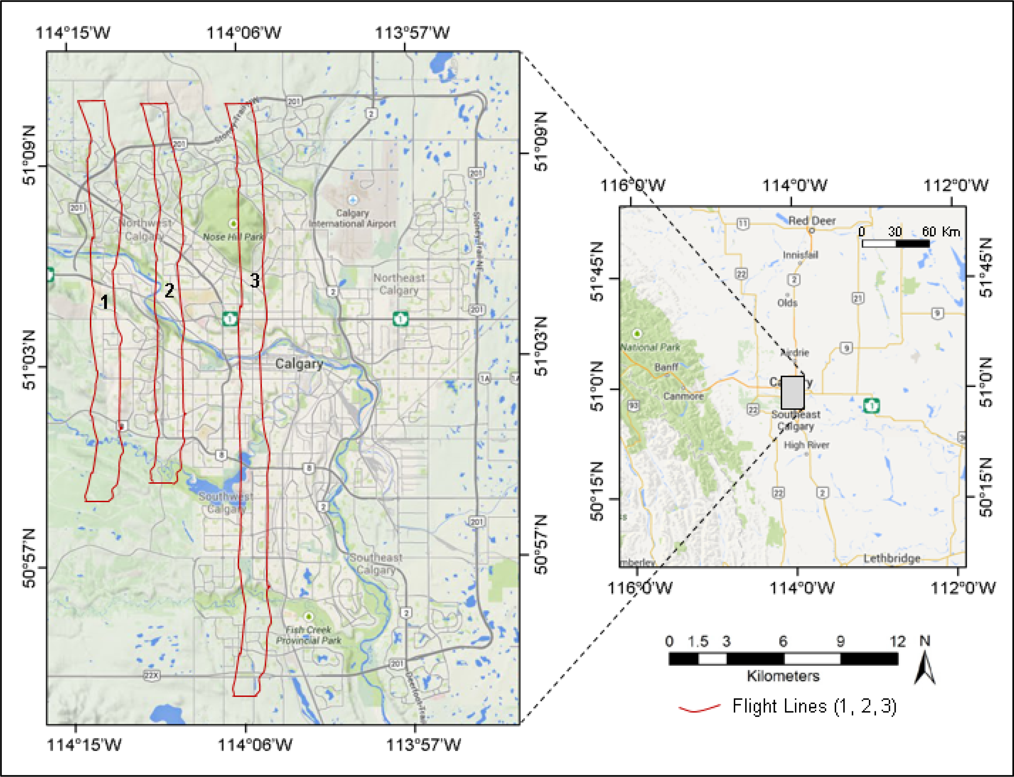
Our study area consists of three non-adjacent H-Res TIR flight-lines (Figure 1) that were extracted for analysis from a full City of Calgary TABI-1800 (Thermal Airborne Broadband Imager) dataset (∼825 km2) composed of 43 flight-lines (∼600 GB). These three flight-lines were acquired during the night (between 00:00 and 04:30) on 13 May 2012 and cover a heterogeneous urban area of ∼182 km2 at a 50 cm spatial resolution. During their acquisition, the ambient night-time temperature ranged from 8 to 13 °C and winds ranged from 5 to 13 km/hr., gusting to 20 km. Local weather data were accessed from 26 reporting sites available from the Weather Underground ( http://www.wunderground.com - last accessed 6 June 2014).
The TABI-1800 is a recent (circa 2012) airborne thermal infrared sensor with a swath width of 1800 pixels in the 3.7–4.8 µm spectral region, a thermal resolution of 0.05 °C, and the ability to collect up to 175 km2 per hour at 1.0 m spatial resolution [26]. This is three to five times faster than most other airborne TIR sensors [14]. In this study, since data were collected at a 50 cm spatial resolution, a nominal swath of 900 m was acquired per flight-line. All flight-lines were orthorectified by the service provider (ITRES Research LTD) using a 10 m digital elevation model (DEM), and the reported geometric accuracy of the dataset was ±1 m. The City of Calgary also provided an RGB-NIR (Red, Green, Blue, Near Infra-red) orthorectified airphoto-mosaic (acquired in 2012, at a 25 cm spatial resolution, geometric accuracy ± 25 cm) and a GIS Road dataset (geometric accuracy ± 25 cm)—composed of polylines that represented road centers. Based ease of use, the TABI data were resampled to 1.0 m using bilinear interpolation. Similarly, the City ortho-mosaic was resampled to a 1.0 m spatial resolution using cubic-convolution (CC). This was based on visual results and the fact that CC models a 4 × 4 area around the central pixel; which corresponds nicely to resampling the scene from 25 cm to 1.0 m.
3. Methods
Caveat: In the proceeding section, we describe TURN (the method) applied only to a single flight-line of TABI-1800 data. Once this entire process has been described, we then repeat the method (Sections 3.2–3.6) on the remaining two non-adjacent flight-lines and present the results of all three flight-lines in the Results and Discussion sections. This is to minimize repetition in the Methods section and to illustrate that TURN can be applied to independently collected H-Res TABI-1800 flight-lines of different data-volumes and acquisition times.
3.1. Pseudo Invariant Features and Mode Road Temperature
To develop the Thermal Urban Road Normalization (TURN) method, road objects (Roads) are considered as pseudo invariant features [27]. This is because: (i) roads are relatively well distributed over modern urban environments, (ii) their primary construction materials are generally the same for different major road types within a given city, thus providing consistent thermal properties [28], and (iii) previous research has revealed a strong correlation between night-time air temperature and road surface temperature [29,30], from which we assume that the road temperature can be used to model urban microclimatic variability in terms of energy flux.
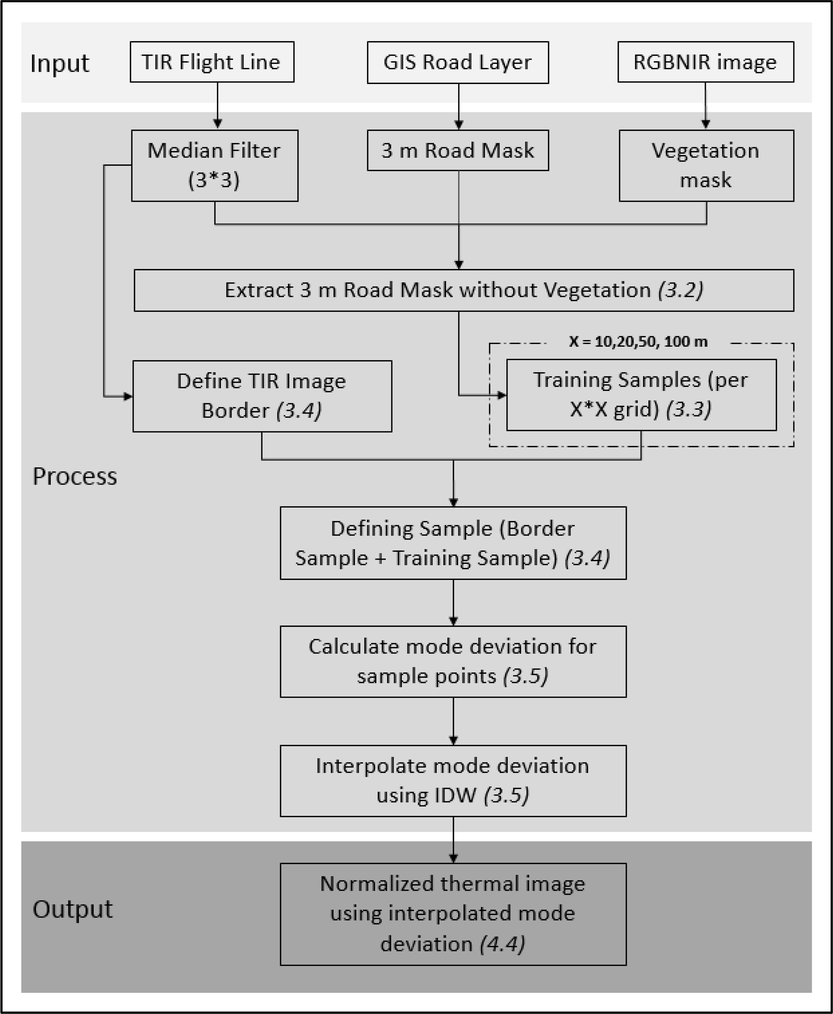
As the TIR imagery were acquired late at night, any variation from the (mode) Road temperature within a flight-line is considered the result of local microclimatic variability. Based on these conditions, the TURN method consists of extracting an object Road class from a TIR flight-line, calculating its deviation (see Section 3.5 for details), and interpolating it over the entire TIR flight-line to create a temperature variability surface. This surface can then be used to minimize the impact of microclimate variability on other object classes present in the TIR flight-line. We note that object/shape-based interpolation techniques are also commonly used in medical imaging to fill voids in an image [31–33]. Building on these ideas we use similar techniques to create a continuous, smooth microclimatic variability map. The flowchart in Figure 2 briefly outlines this methodology which is further described in detail in the proceeding sections (3.2–3.6).
3.2. Road Extraction
A global road class (Road) is extracted from the TIR flight-line based on The City GIS Road data. These data represent the road center-lines of four different road types: (i) primary, (ii) secondary, (iii) access, and (iv) back-alleys. In this study, only primary and secondary roads are considered. This is because in Calgary, they are typically composed of asphalt. Back-alleys and access roads are omitted as they are typically covered by trees, and are composed of numerous mixed materials (e.g., gravel, clay, brick, asphalt, cement and others), many of which have difficult-to-define thermal characteristics.
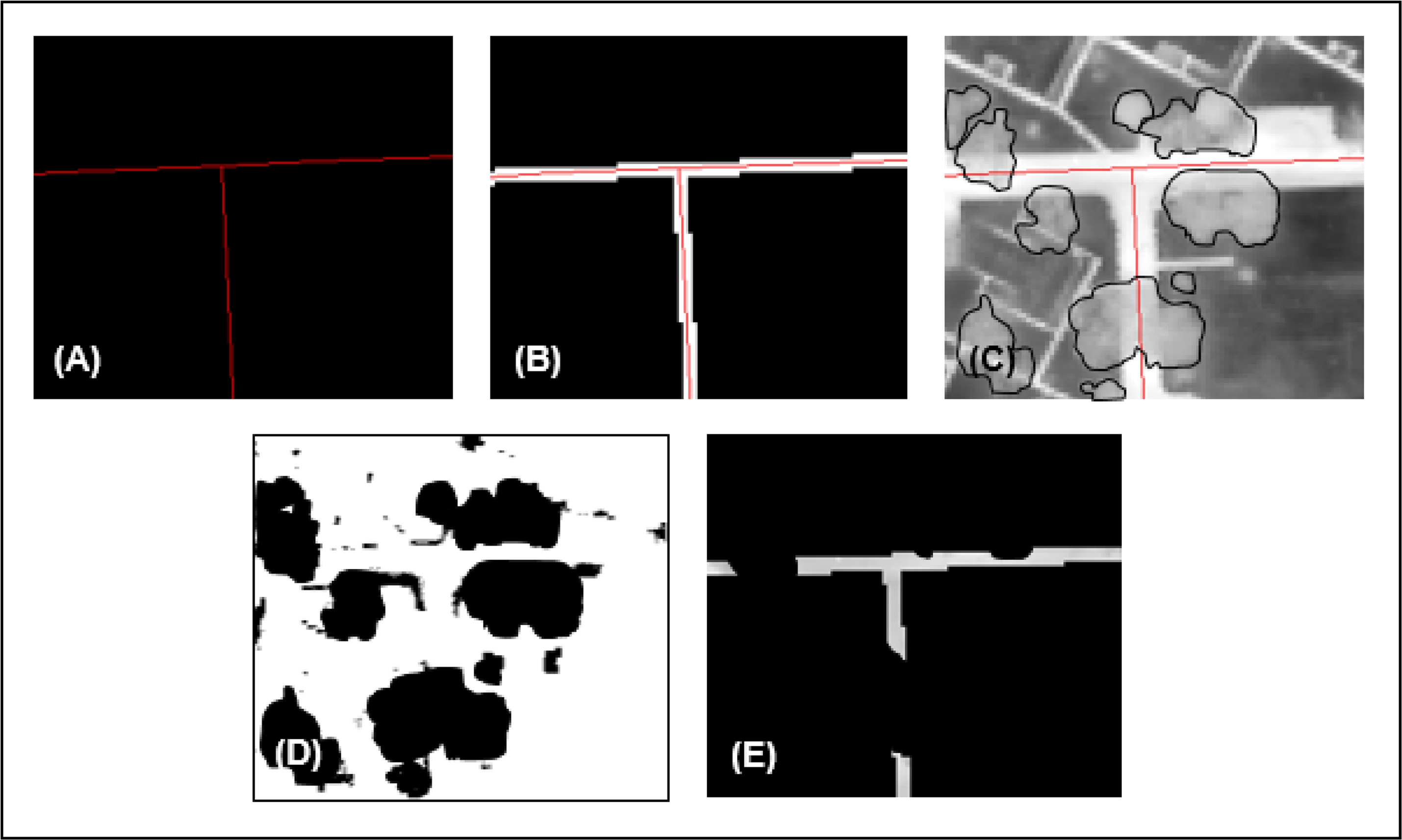
To extract the Road class, we first apply a 3 × 3 median filter to the TIR image to reduce noise and simplify the scene. We then create a 1.5 m buffer on each side of the GIS Road center (Figure 3A) to produce a 3.0 m wide Road mask (Figure 3B). A 3.0 m section along the road center was chosen based on (i) a minimum Calgary road width (∼10 m) and (ii) the ability to avoid sampling vehicles parked along the sides of the road (∼2.5–3.5 m). The Road mask is then combined with the TIR image to extract the central portions of the corresponding roads. A visual inspection reveals that portions of many roads are covered by trees (Figure 3C). To eliminate these, a vegetation mask (Figure 3D) is created by calculating an NDVI (from the 1.0 m RGB-NIR ortho-photo), then quickly manually thresholding it based on visual inspection. Once defined, this vegetation mask is then dilated by 1.0 m to compensate for possible geometric error between the RGB-NIR and the TIR image. This dilated vegetation mask is then applied to the 3.0 m Road class to eliminate overhanging vegetation (Figure 3E).
Next, a histogram of the extracted Road class (Figure 4A) is created to visually and statistically assess any remaining road temperature noise. Here noise refers to pixels that are not representative of the Road class. From Figure 4, we see that the histogram has a bimodal distribution. When linked to the corresponding thermal flight-line, we are able to determine that the left distribution is primarily representative of gravel roads, road construction, and vehicles, which we denote as noise (Figure 4B). In an effort to automate the process of reducing this noise, we examined many different combinations of mean (µ) and standard deviation (σ) (derived from each flight-line) to determine an optimum range of noise DNs. Analysis revealed that a range of (µ − 2σ) to (µ + 3σ) best represents the Road class with minimum noise. Therefore, the DNs beyond this range (the noise) were masked out, and the remaining road pixels were used for further processing. We note that this noise minimizing technique was evaluated on all three flight-lines separately and was observed to work well on each of them. As a result, we are confident that this noise removing technique is sufficiently robust to be automated—at least for this full-city dataset.
3.3. Multi-Interval Sampling
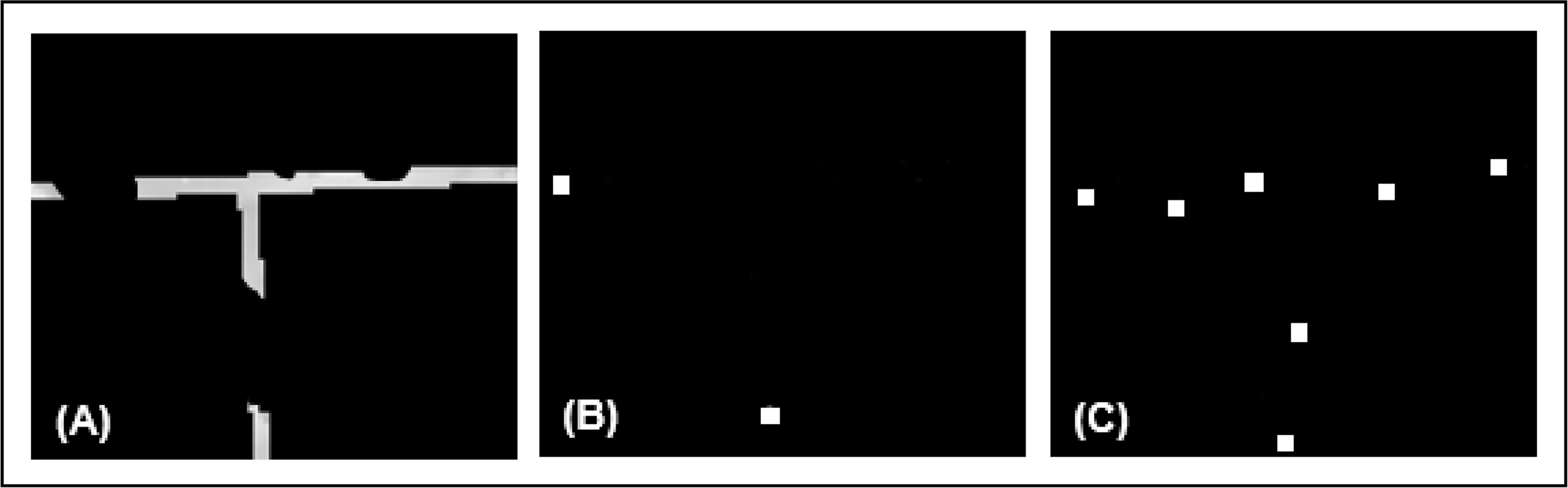
Of all the Road pixels defined in Section 3.2, 0.5% of each flight-line (totaling ∼1800–2400 pixels, depending on the size of the flight-line) are randomly selected and saved as a test dataset for accuracy assessment (Figure 5A–C). The remaining Road pixels (99.5%) are used for analysis.
At a 1.0 m spatial resolution, a 3.0 m wide section of the Road mask (Figure 5A) distributed over each flight-line contains many spatially adjacent and spectrally similar pixels, making spatial interpolation challenging. Furthermore, due to the varying size, shape and orientation of Road objects, it is not possible to determine an optimal sample interval using statistical autocorrelation. To simplify this interpolation problem, we divide the entire flight-line into X*X m grid cells (X = 10, 20, 50, and 100 m) and select one representative Road pixel from each cell, which we define as the median value of all sampled Road pixels within each grid cell. The median is selected rather than mode, as it is possible that all samples within a grid cell are unique. We also retain each median Road DN at its actual sampled location, rather than arbitrarily placing it at the center of an X*X cell—as the cell center may be located far from the road. These Road samples (Figure 5C) are then used for further processing. In this paper, we evaluate this sampling technique at four (X) different sampling intervals (10, 20, 50, and 100 m) to determine the optimum sampling strategy (see Section 3.4 for details).
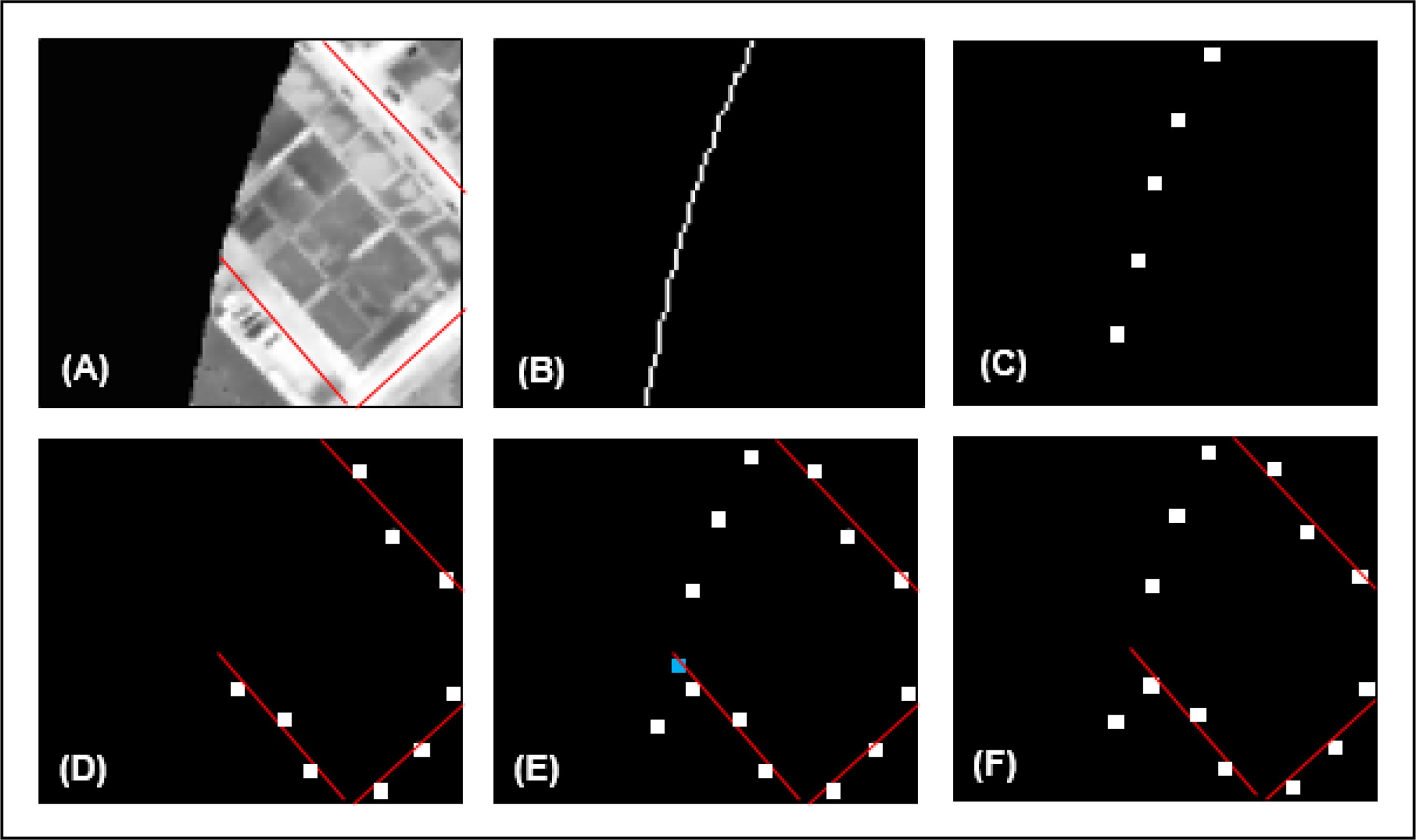
3.4. Sample Optimization: Boarders and Oversampling
Airborne data are seldom acquired in perfect straight lines. Consequently, the border of such data are often padded with zero values to ensure a rectangular shape of the output flight-line (Figure 6A). To tie the interpolated TURN-surface to this edge, its boundary is detected using a Laplacian edge detection filter (Figure 6B) and sample points are taken along its border at 10 m intervals (Figure 6C). In this section we describe sample optimization at 10 m intervals. Later, the same process is repeated for 20, 50, and 100 m intervals and the results are described in Section 4. For parsimony, the border samples are then assigned the values of the closest Road sample (Figure 6D) and are combined with the samples generated in step 3.3 (Figure 6E). Next, a cleaning filter is applied over all flight-line samples so that a maximum of one sample point exists within a 10*10 m window (Figure 6F). Cleaning is performed to avoid oversampling of points. The remaining sample points are then interpolated to create a (continuous) Road temperature variability surface (a TURN-surface) over the entire flight-line.
3.5. Spatial Interpolation of Road Temperature Variations
Our objective with these samples, is to interpolate Road temperature deviation as a smooth and continuous surface for each flight-line. Conceptually, this surface represents variation in land surface temperature within a flight-line due to the nonlinear interaction of local microclimatic components (i.e., wind, precipitation, and humidity). To create this surface, we first calculate the mode Road temperature from the Road class generated in step 3.2. From a statistical perspective, we consider the mode of Road temperature samples of a TIR flight-line as the most representative temperature of all Roads (rather than the average) as it occurs most frequently throughout the flight-line; thus it is the most ‘road-like’. We then collect TIR road training samples (steps 3.3–3.4), and then, for each sample we calculate the local mode deviation (Dij) using Equation (1). These mode deviation values are then interpolated over the entire flight-line using Inverse Distance Weighting (IDW) [33]. Specific interpolation parameters includes: (i) Maximum search radius = 100 m, (ii) Minimum number of closest points used for each local fit = 3, and (iii) Smoothing radius = 10 m
Dij = Mode deviation at pixel (i, j)
Xij = Radiant temperature of pixel (i, j)
X = Mode Road temperature for a given flight-line
We note that prior to selecting IDW, seven different interpolation techniques were visually and statistically evaluated [34]. These included: (i) Splines [35], (ii) Nearest Neighborhood [36], (iii) Polynomial [37], (iv) Kriging [38], (v) Inverse Distance Weighted (IDW), (vi) Triangular Integrated Network (TIN) [39], and (vii) Radial Basis Function (RBF) [40]. Based on our visual and statistical assessment of the resulting surfaces, IDW produced the smoothest appearing surface based on locally varying values; which is consistent with the conceptual models of locally explicit, but regionally continuous microclimatic variability [29,30]. Therefore, we have used IDW interpolation for the remainder of this analysis.
In this study, we consider the interpolated deviation surface to represent temperature differences in a flight-line resulting from local microclimatic variations. Conceptually, this surface can be used to normalize the effect of microclimate within the original thermal flight-line using Equation (2), where the interpolated variability map is simply subtracted from the thermal flight-line:
Nij = Normalized radiant temperature of pixel (i, j)
Dij = Mode deviation at pixel (i, j)
Xij = Original radiant temperature of pixel (i, j)
In reality, an emissivity correction (of the Road class, as well as all other land cover classes in the flight-line) might be performed prior to interpolation and normalization, similar to the emissivity modulation (EM) method described by Nicole [41]. Depending on the physical properties of an object, it emits only a portion of its absorbed energy. Emissivity expresses the ability of an object to emit radiant energy [42]. If not corrected for emissivity, TURN only provides a radiant thermal microclimate normalization of the scene—see Section 4.5.3 for details on EM and emissivity.
3.6. Validation of the Method
Once the original flight-lines are normalized for microclimatic variability using Road temperature deviation, an accuracy assessment is performed to evaluate the performance of the method. It is expected that the radiant Road temperatures over an entire flight-line will be equal to the mode Road temperature after applying TURN. To verify this, the temperature of the test Road pixels (step 3.2) before and after normalization were compared using the Root Mean Square Error (RMSE) which is calculated using Equation (3):
X = Mode Road temperature of a flight-line
Xij = Road temperature of pixel (i, j)
n = Number of total test pixels
In this experiment, the RMSE essentially describes how the radiometric variability of similar objects (i.e., samples derived from a ‘homogeneous’ road class) change after applying TURN. Lower RMSE values represent more ‘object-like’ results, thus our goal is to obtain a lower RMSE result for the same (Road) class. This is because image-objects by definition [43] tend to be composed of similar components (i.e., pixels with similar DN values), thus they have a lower internal variability.
4. Results and Discussions
The Methods section described TURN applied to a single TIR flight-line based on a 10 m sampling interval. In this section, we describe and discuss the results of the same method independently applied to all three thermal flight-lines (shown in Figure 1) over four different sampling intervals (10, 20, 50, and 100 m). Table 1 outlines the size of the flight-lines, the number of training samples for each sampling interval, and the number of test (Road) pixels used for accuracy assessment.
The following sections (4.1–4.4) discuss and compare the results generated from these flight-lines at different sampling intervals. Section 4.5 discusses operation considerations, errors and uncertainties and Section 4.6 discusses the importance of incorporating existing GIS image-objects into the GEOBIA workflow.
4.1. Sample Size vs. Processing Time
As automation and operationalization of the TURN method are important goals of this research, we compared the processing speeds for collecting and interpolating samples at different sampling intervals for different sized flight-lines. To do so, we ran TURN with the same workstation (Intel® Core ™ i7-2600, Windows Server 2008 (64 bit) on a Quad Core CPU at 3.40GHz, RAM: 16 GB) on each of the three flight-lines for four different sampling intervals. TURN code is written in Interactive Data Language (IDL 8.0, 64 bit version). Figure 7 and Table 1 show that as the Road sample interval (i.e., distance between adjacent samples) for each flight-line decreases, the number of samples and the required processing time increases.
If we consider the results shown in Figure 7 and were to extrapolate them to process the entire City of Calgary TIR scene (which consists of 43 TABI-1800 flight-lines covering ∼825 km2 and a data volume of ∼600GB), we estimate that it will require ∼7 hours to process all flight-lines at the 10 m sampling interval, ∼5 hours for the 20 m sampling interval, ∼2.5 hours for the 50 m sampling interval, and ∼1.2 hours for the 100 m sampling interval. Thus, the processing time is negatively correlated with the sampling interval (i.e., the larger the sampling interval, the less processing time involved). We also note that flight-line 3 requires considerably more processing time than the other flight-lines, as it is ∼50% larger (in size) than the other two flight-lines that were evaluated (see Table 1 and Figure 1).
4.2. An Assessment of Radiometric Normalization Accuracy Based on RMSE
We consider the mode Road temperature of each independent flight-line as its reference temperature, and radiometrically normalize the thermal flight-line to this mode as it represents the most abundant temperature within the flight-line. Therefore, we expect that after normalization, Road temperatures within a flight-line will shift to its mode temperature. To test this hypothesis, we randomly selected a number of Road test pixels from the original flight-lines (see Table 1) and evaluated their RMSE with corresponding samples from the normalized mode Road temperature scenes to determine their radiometric similarity (in °C). Conceptually, the smaller the RMSE, the closer the Road temperature is to the mode Road temperature, meaning that the effects of microclimate are increasingly normalized.
In order to best illustrate the effects of all four different sample intervals on each of the 3 flight-lines, Figure 8 shows the percent decrease in RMSE - where larger values are better. This is because they represent a greater reduction in RMSE between the original image and the normalized image. In all cases, the RMSE decreases after normalization, thus the road temperatures are becoming more consistent across the scene, as per our initial assumption. However, the normalized test pixels are closest to the mode Road temperature for TURN-surfaces generated from small sampling intervals. This means that greater overall similarity is achieved for smaller sample sizes; though we note that statistically, the percentage difference is relatively small (∼2–3%) between the 10 m, 20 m and 50 m sample intervals. In contrast, the 100 m sample shows a notable decrease (4–7%) in RMSE compared to the 10 m sample, indicating that microclimatic variability is less well (statistically) modeled at this coarser sampling interval.
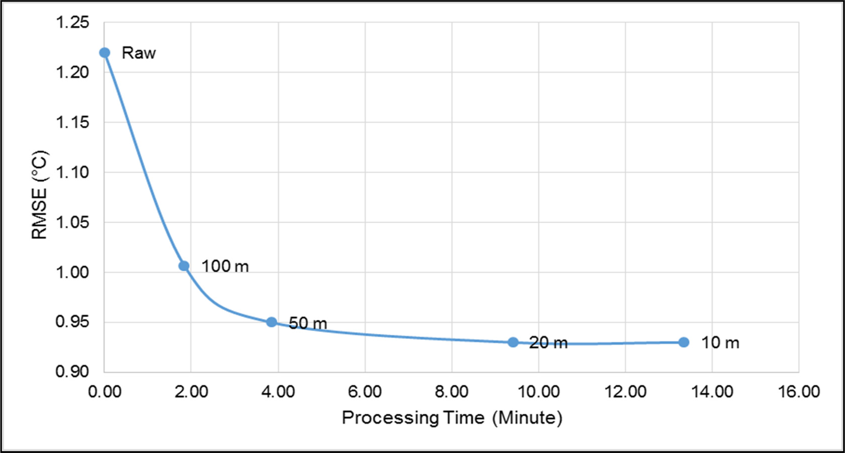
4.3. Root Mean Square Error (RMSE) vs. Processing Time
Considering the fact that TURN is developed for large-area high-spatial resolution (1.0 m) TIR imagery, processing needs to be fast while also maintaining a strong reduction in RMSE. To compare accuracy (RMSE) vs. processing time, we calculated the mean decrease in RMSE and mean processing time of three flight-lines for four different sampling intervals and plotted them (Figure 9).
Results show that as the sampling interval decreases, the accuracy increases (thus the RMSE gets smaller), but the processing time also increases. However, we note that between the 10 m and 20 m sample intervals, processing time decreased by ∼30%, but statistically, the average accuracy did not change noticeably. Conversely, the processing time for the 100 m sample interval is 85% less than at the 10 m sampling interval. However, its average accuracy is considerably decreased (∼7%). Considering these results, we conclude that 20 m is the optimum sample interval for this study, as it balances local temperature variability (Figure 10) and computation speed.
4.4. Visual Assessment of Interpolated Surfaces at Different Sampling Intervals
TURN generates an interpolated surface representing the Road temperature deviations within a flight-line. Figure 10 provides an example of how microclimate variability is visually represented by the TURN-surface at different sampling intervals.
The flight-line sample in Figure 10A represents two main vegetated areas (one at the top and another at the middle of the figure) surrounded by roads and buildings. From a detailed visual inspection, we note that the vegetated areas are cooler than the built-up areas, making the adjacent roads appear cooler (dark grey) than the mode Road temperature; thus, requiring a positive temperature adjustment (i.e., see the light grey surfaces at the top and middle of Figure 10B). Figure 10B,C shows that the thermal characteristics of different land cover types are visually represented in greater detail with 10 m and 20 m sampling intervals. At the 50 m sampling interval (Figure 10D), the surface is more generalized, but still sufficient to distinguish different types of land cover (compared with Figure 10A). However, at the 100 m sampling interval (Figure 10E), a larger portion of the corresponding land surface temperature detail is lost through generalization. We note that, given these unique perspectives, TURN-surfaces may also represent useful tools for urban planners to identify potential urban heat sinks, and localized sources of urban heat islands.
The idealized final output of the proposed model is a flight-line ‘free’ from the effects of microclimate, thus displaying a more uniform radiometric response of similar objects within it. In Figure 11, we show an example of how radiometric difference among similar objects decreases after applying TURN. Figure 11A represents a portion of the raw flight-line displaying rooftop, road, grass, etc., Figure 11B represents the TURN-surface created using 10 m sampling interval, and Figure 11C represents the normalized portion of the flight-line using TURN-surface. If we look at the rooftops in the raw image (Figure 11A), we notice that they are represented by different shades of blue and green meaning that there is a notable variation in rooftop temperature. However, once TURN applied (Figure 11C), the rooftops appear much consistent (green).
4.5. Operational Considerations, Errors and Uncertainties
This section briefly discusses three important operational consideration regarding TURN.
4.5.1. Mitigating Microclimate, Surface and Atmospheric Effects
When acquiring TIR airborne imagery, ideally winds should be lower than 5–10 km/hr and ambient temperate lower than 7 °C so as to provide sufficient environmental contrast [44]. However, the reality is that weather is dynamic, and even the best planned acquisitions need to deal with the often changing meteorological conditions they are presented with. This in part is why TURN was conceived, and why we suggest it will become an important contribution to the TIR community. We further propose that given sufficient spatial and temperature resolution to define appropriate road samples, the TURN method is able to visually and statistically mitigate the integrated impact of microclimatic and atmospheric variability and other physical surface conditions such as elevation, slope, aspect etc. that externally influence TIR radiometry acquired from H-Res TIR platforms [14,15]. This is because the temperatures derived from local road samples already represent an integration of these environmental conditions. Nevertheless, evidence of this is beyond the scope of this research. As noted in Section 2, we do have access to temperature data from 26 meteorological stations during the TIR acquisition time. However, for a large city like Calgary (∼43 TABI-1800 TIR flight-lines), we suggest that 26 stations is simply too coarse to validate microclimatic variability, which occurs within 1–100 m. To do so, would require setting up ∼40–60 meteorological stations (1 every km2) within each flight-line, and ∼800–1000 stations for the whole city; which is beyond the scope of this—or any study that we are aware of.
4.5.2. Road Pseudo-Invariance
TURN is developed based on the assumption that roads of the same material are radiometrically invariant. In reality, roads are not completely invariant due to their different material types and surface conditions (resulting from age, traffic load, exposure to solar radiation, geographic location, etc.) [45]. However, this is also true for all other pseudo-invariant features [27]. Conceptually, for this project, this situation can only be avoided by manually acquiring numerous road temperature samples over the entire study area, immediately prior to TIR data collection (to allow for them to reach thermal equilibrium with the environment), which is completely impractical for large study areas. This in-part is why this method was developed.
4.5.3. Emissivity Corrections
The three evaluated flight-lines represent the radiant temperature of different land cover composing the scene. Thus, Road extraction and interpolation are also performed based on radiant temperatures. For absolute microclimate temperature corrections, emissivity corrected Road samples need to be interpolated and applied to an emissivity corrected surface. For example, Nichol [41] proposed the Emissivity Modulation (EM) technique (similar to image sharpening described by Gustavson et al. [46]) to correct thermal images for different emissivity classes. EM uses a geographically corrected optical image to classify different land cover classes. The corresponding emissivity class values are then integrated with the thermal image to calculate true kinetic temperature. Based on this idea, we suggest that EM along with TURN can be used to produce an emissivity corrected and microclimate normalized TIR flight-line that represents the true kinetic temperature of the cover-types of interest.
4.6. Transforming Existing Vector Image-Objects into Multiscale Fields
Bain [47] describes three main categories of geographic space—spatial objects, regions, and fields—and notes that fields are not well represented by objects. However, to the best of our knowledge, this is the first time in the GEOBIA literature, that discrete sparsely sampled image-objects are transformed into a continuously varying multiscale field. To do so, we initially define roads by buffering around existing City of Calgary GIS vectors (i.e., polylines) that represent road centers. Thus, we do not actually apply segmentation to define the initial road objects (though we do apply thresholding to an NDVI image to remove vegetation objects that overhang/obscure these new road-objects). In this sense, TURN is a step towards meeting a recent challenge to the GEOBIA community [48] to incorporate existing GIS vector objects within the GEOBIA workflow, rather than relying solely on segmentation methods that have no unique solution [25].
5. Conclusions
Local microclimatic components such as wind, humidity, precipitation and surface moisture have a non-linear impact on TIR imaging, making detailed analysis non-trivial. To mitigate these effects, we describe Thermal Urban Road Normalization (TURN) applied to three non-adjacent flight-lines of H-Res TABI-1800 imagery (∼182 km2), that cover a complex urban scene. TURN is a new method that radiometrically normalizes TIR flight-lines so that it appears as if the entire scene were acquired under the same microclimate conditions and at the same time. In this method, roads within the scene are considered as a pseudo invariant feature from which (environmentally integrated) temperature samples are defined and interpolated. Road samples are used as a reference object-class for two reasons: (i) Road material is generally constant within a city, and (ii) Roads are relatively evenly distributed over urban areas—thus providing a sufficient number of evenly distributed samples from which to create a continuous interpolated TURN-surface. This TURN-surface is a continuous temperature variability map, that models (i) the integrated effects of microclimatic variability over the entire TIR scene, and (we also suggest), (ii) location-based characteristics such as elevation, slope and aspect, and (iii) atmospheric variability, as these characteristics are already integrated within the extracted TIR samples.
We note that prior to interpolation, eight different spatial interpolation techniques (Section 3.5) were evaluated, with Inverse Distance Weighting (IDW) generating the most representative surface, as it specifically models the influence of local variability. The resulting TURN-surface (derived using IDW) is then used to normalize the original TIR flight-line by removing the varying effects of local microclimate. In total, radiometric normalization was performed on three non-adjacent flight-lines at four different sample intervals (10 m, 20 m, 50 m, and 100 m). Results show that as the normalization interval decreased, the accuracy increased (i.e., the internal variability of similar features within a thermal flight-line decreased). Specifically, this method reduced the internal Road temperature variability by ∼25% at the 10 m and 20 m sampling interval, ∼19% at the 50 m sampling interval, and ∼15% at the 100 m sampling interval. However, as the sampling interval decreased, the processing time increased. From the combined results of reduced within-scene variability and computational speed, we conclude that 20 m is the optimum sampling scheme to generate a TURN-surface, as: (i) processing time is reduced by ∼25% (compared to that at 10 m), (ii) the radiometric normalization accuracy (RMSE) changed very little compared to results achieved at 10 m, and (iii) the 20 m temperature variability map showed very similar radiometric detail to that of 10 m.
While these results are very promising, we note that in some circumstances it may be a challenge to define specific road-types as pseudo invariant features. This is because the radiometry of general road-types depends upon material type, age, surface condition, orientation and surrounding environment. Thus, care should be applied when selecting appropriate roads. However, this does not invalidate the selection of road-types in this evaluation, as GIS road-types were provide by the City of Calgary. Another cautionary note, involves the lack of sufficient field data to validate the model at fine resolutions. Although samples from 26 weather stations were available for the entire City of Calgary during this acquisition, this sample size is insufficient for large area validation. Thus, the next step of this research includes validating the TURN model in a smaller pilot site using extensive field measurements. However, we note that it is not trivial to obtain extensive road/air temperature measures coincident with a TIR airborne acquisition; which in-part, is why this method was initially developed. In addition, even if sufficient measures were obtained, they would only validate the method applied to a relatively small number of samples.
Thermal Urban Road Normalization (TURN) is a new method that enables the generation of radiometrically uniform flight-lines, so that physically similar features within a flight-line exhibit consistent temperatures. Furthermore,
▪ This method can be automated, is computationally fast and highly transferable; thus we propose that it is able to be operationally applied to large, H-Res TIR datasets.
▪ TURN-surfaces may represent a useful tool for urban planners to identify urban heat sinks, and localized sources of urban heat islands.
▪ Conceptually, TURN-surfaces could be integrated with the Emissivity Modulation method [41] to produce an emissivity corrected and microclimate normalized TIR scene that represents the true kinetic temperature of the corresponding cover-types of interest.
▪ To the best of our knowledge, this is the first time in the GEOBIA literature, that discrete road-objects are defined and sampled to create a continuous temperature variability field for the full-scene, which is then used to automatically obtain a ‘microclimate-free’ scene.
▪ This research meets a recent challenge to the GEOBIA community to integrate pre-defined GIS vector objects within the analytical process rather than solely defining image-objects with segmentation methods that have no unique solution.
Acknowledgments
We acknowledge support from The Institute for Sustainable Energy, Environment and Economy ( www.iseee.ca), ITRES Research Limited ( www.itres.com), The City of Calgary ( www.calgary.ca), Tecterra ( www.tecterra.com), NSERC ( www.nserc.ca), The Alberta Real Estate Foundation ( www.aref.ab.ca) and the Calgary Real Estate Board ( www.creb.com). We also acknowledge a University of Calgary Faculty Graduate Research Scholarship and a Geography Excellence Award provided to Mir Mustafizur Rahman, and an Alberta Informatics Circle of Research Excellence (iCore) MSc Scholarship and an ISEEE Graduate Scholarship awarded to Bharanidharan Hemachandran.
Author Contributions
Mir Mustafizur Rahman processed the thermal and the optical data, analyzed the results, wrote the paper, and is the main author of the article. Geoffrey J. Hay helped with ideas and technical advices during the development stage of the algorithm and also contributed in reviewing the paper. Isabelle Couloigner helped in editing the paper, and Bharanidharan Hemachandran contributed in collecting and processing ground weather station data.
Conflicts of Interest
One of the co-authors (G. J. Hay) of this paper is a co-editor of the special issue (Advances in Geographic Object-Based Image Analysis) to which this paper is submitted.
References
- Prakash, A. Thermal remote sensing: Concepts, issues and applications. Int. Arch. Photogramm. Remote Sens 2000, 33, B1. [Google Scholar]
- Kidder, S.Q.; Wu, H.T. A multispectral study of the St. Louis area under snow-covered conditions using NOAA-7 AVHRR data. Remote Sens. Environ 1987, 22, 159–172. [Google Scholar]
- Roth, M.; Oke, T.R.; Emery, W.J. Satellite-derived urban heat island from three coastal cities and the utilization of such data in urban climatology. Int. J. Remote Sens 1989, 10, 1699–1720. [Google Scholar]
- Kim, H.H. Urban heat island. Int. J. Remote Sens 1992, 13, 2319–2336. [Google Scholar]
- Gallo, K.P.; Owen, T.W. Assessment of urban heat island: A multi-sensor perspective for the Dallas-Ft. Worth, USA region. Geocarto Int 1998, 13, 35–41. [Google Scholar]
- Streutker, D.R. A remote sensing study of the urban heat island of Houston, Texas. Int. J. Remote Sens 2002, 23, 2595–2608. [Google Scholar]
- Pozo, D.; Olrno, F.J.; Alados-Arboledas, L. Fire detection and growth monitoring using a multitemporal technique on AVHRR mid-infrared and thermal channels. Remote Sens. Environ 1997, 60, 111–120. [Google Scholar]
- Voogt, J.A.; Oke, T.R. Complete urban surface temperatures. J. Appl. Meteorol 1997, 36, 1117–1132. [Google Scholar]
- Quattrochi, D.A.; Ridd, M.K. Analysis of vegetation within a semi-arid urban environment using high spatial resolution airborne thermal infrared remote sensing data. Atmos. Environ 1998, 32, 19–33. [Google Scholar]
- King, M.D.; Menzel, W.P.; Kaufman, Y.J.; Tanre, D.; Gao, B.C.; Platnick, S.; Ackerman, S.A.; Remer, L.A.; Pincus, R.; Hubanks, P.A. Cloud and aerosol properties, precipitable water, and profiles of temperature and water vapor from MODIS. IEEE Trans. Geosci. Remote Sens 2003, 41, 442–458. [Google Scholar]
- Gonzalez, J.E.; Luvall, J.C.; Rickman, D.; Comarazamy, D.; Picon, A.J.; Harmsen, E.W.; Parsiani, H.; Ramirez, N.; Vasquez, RE.; Williams, R.; Waide, R.B.; Tepley, C.A. Urban heat islands developing in coastal tropical cities. Eos Trans. AGU 2005, 86, 397–403. [Google Scholar]
- Pu, R.; Gong, P.; Michishita, R.; Sasagawa, T. Assessment of mult-resolution and mulit-sensor data for urban surface temperature retrieval. Remote Sens. Environ 2006, 104, 211–225. [Google Scholar]
- Gluch, R.; Quattrochi, D.A.; Luvall, J.C. Multi-scale approach to urban thermal analysis. Remote Sens. Environ 2006, 104, 123–132. [Google Scholar]
- Hay, G.J.; Kyle, C.; Hemachandran, B.; Chen, G.; Rahman, M.M.; Fung, T.S.; Arvai, J.L. Geospatial technologies to improve urban energy efficiency. Remote Sens 2011, 3, 1380–1405. [Google Scholar]
- Rahman, M.M.; Hay, G.J.; Couloigner, I.; Hemachandran, B.; Bailin, J.; Zhang, Y.; Tam, A. Geographic Object-Based Mosaicing (OBM) of high-resolution thermal airborne imagery (TABI-1800) to improve the interpretation of urban image objects. IEEE Geosci. Remote Sens. Lett 2013, 10, 918–922. [Google Scholar]
- Quattrochi, D.A.; Luvall, J.C. Thermal infrared remote sensing for analysis of landscape ecological processes: methods and applications. Landscape Ecol 1999, 14, 577–598. [Google Scholar]
- Hartz, D.A.; Prashad, L.; Golden, J.; Brazel, A. J. Linking satellite images and hand held infrared thermography to observe neighborhood climate conditions. Remote Sens. Environ 2006, 104, 190–200. [Google Scholar]
- Santamouris, M.; Papanikolaou, N.; Livada, I.; Koronakis, I.; Georgakis, A.; Assimakopoulos, D.N. On the impact of urban climate on the energy consumption of buildings. Solar Energy 2001, 70, 201–216. [Google Scholar]
- Giannini, A.; Saravanan, R.; Chang, P. Oceanic forcing on sahel rainfall on interannual to interdecade time scales. Science 2003, 302, 1027–1030. [Google Scholar]
- Voogt, J.A.; Oke, T.R. Thermal remote sensing of urban climates. Remote Sens. Environ 2003, 86, 370–384. [Google Scholar]
- Friedl, M.A.; Davis, F.W. Sources of variation in radiometric surface temperature over a tallgrass prairie. Remote Sens. Environ 1994, 48, 1–17. [Google Scholar]
- Lagouarde, J.P.; Ballans, H.; Moreau, P.; Guyon, D.; Coraboeuf, D. Experimental study of brightness surface temperature angular variations of maritime pine (Pinus pinaster) stands. Remote Sens. Environ 2000, 72, 17–34. [Google Scholar]
- Crippen, R.E.; Hook, S.J.; Fielding, E.J. Nighttime ASTER thermal imagery as an elevation surrogate for filling SRTM DEM voids. Geophys. Res. Lett 2007, 34, L01302. [Google Scholar]
- Blaschke, T.; Hay, G.J.; Maggi, K.; Lang, S.; Hofmann, P.; Addink, E.; Feitosa, R.Q.; van der Meer, F.; van der Werff, H.; Coillie, F.V. Geographic Object-Based Image Analysis—Towards a new paradigm. ISPRS J. Photogramm. Remote Sens 2014, 87, 180–191. [Google Scholar]
- Hay, G.J.; Castilla, G. Geographic Object-Based Image Analysis GEOBIA: A new name for a new discipline? In Object-Based Image Analysis: Spatial Concepts for Knowledge-Driven Remote Sensing Applications; Blaschke, T., Lang, S., Hay, G.J., Eds.; Springer-Verlag: New York, NY, USA, 2008; Chapter 1.4; pp. 81–92. [Google Scholar]
- ITRES, 2014. Available online: http://www.itres.com/ (accessed on 13 June 2014).
- Schott, J.R.; Salvaggio, C.; Volchok, W.J. Radiometric scene normalization using pseudo invariant features. Remote Sens. Environ 1988, 26, 1–14. [Google Scholar]
- The City of Calgary. In Road Construction: 2012 Standards and Specifications; ROADS Construction Division, Transportation Department, The City of Calgary: Calgary, AB, Canada, 2012; Available online: http://www.calgary.ca/Transportation/Roads/Pages/Contractors-and-Consultants/Contractors-and-Consultants.aspx (accessed on 5 August 2014).
- Bogren, J.; Gustavsson, T. Nocturnal air and Road surface temperature variations in complex terrain. Int. J. Climatol 1991, 11, 443–455. [Google Scholar]
- Gustavson, T. A study of air and Road-surface temperature variations during clear windy nights. Int. J. Climatol 1994, 15, 919–932. [Google Scholar]
- Herman, G.T.; Zheng, J.; Bucholtz, C.A. Shape-based interpolation. IEEE Comput. Graph. Appl 1992, 12, 69–79. [Google Scholar]
- Grevera, G.J.; Udupa, J.K. Shape-based interpolation of multidimensional grey-level images. IEEE Trans. Medical Imaging 1996, 15, 881–892. [Google Scholar]
- Bors, A.G.; Kechagias, L.; Pitas, I. Binary morphological shape-based interpolation applied to 3-D tooth reconstruction. IEEE Trans. Medical Imaging 2002, 21, 100–108. [Google Scholar]
- Rahman, M.M.; Hay, G.J. Normalizing the effects of local microclimatic and temporal variability in urban thermal airborne imagery. In Proceedings of Canadian Association of Geographers Annual Conference, Calgary, AB, Canada, 31 May–4 June 2011.
- Franke, R. Scattered data interpolation: Tests of some methods. Math. Comp 1982, 38, 181–200. [Google Scholar]
- Parker, J.A.; Kenyon, R.V.; Troxel, D.E. Comparison of interpolating methods for image resampling. IEEE Trans. Medical Imaging 1983, 2, 31–39. [Google Scholar]
- De Boor, C. A Practical Guide to Splines; Springer-Verlag: New York, NY, USA, 1978; Volume 27, p. 368. [Google Scholar]
- Isaaks, E.H.; Srivastava, R.M. An Introduction to Applied Geostatistics; Oxford University Press: New York, NY, USA, 1989. [Google Scholar]
- Renka, R.J.; Cline, A.K. A triangle-based C1 interpolation method. Rocky Mountain J. Math 1984, 14, 223–238. [Google Scholar]
- Franke, R.A. Critical Comparison of Some Methods for Interpolation of Scattered Data; Technical Report; NPS 53-79-003; Naval Postgraduate School: Monterey, CA, USA, 1979. [Google Scholar]
- Nicole, J.E. An emissivity modulation method for spatial enhancement of thermal satellite images in urban heat island analysis. Photgramm. Eng. Remote Sensing 2009, 75, 1–10. [Google Scholar]
- Jacob, F.; Francois, P.; Schmugge, T.; Vermote, E.; French, A.; Ogawa, K. Comparison of Land Surface Emissivity and Radiomatric Temperature Derived from MODIS and ASTER. Remote Sens. Environ 2004, 90, 137–152. [Google Scholar]
- Castilla, G.; Hay, G.J. Image-objects and geo-objects. In Object-Based Image Analysis: Spatial Concepts for Knowledge-Driven Remote Sensing Applications; Blaschke, T., Lang, S., Hay, G.J., Eds.; Springer-Verlag: New York, NY, USA, 2008; Chapter 1.5; pp. 91–110. [Google Scholar]
- Jensen, J. R. Remote Sensing of the Environment: An Earth Resource Perspective, 2nd ed.; Pearson Prentice Hall: Upper Saddle River, NJ, USA, 2007; Chapter 8; pp. 249–290. [Google Scholar]
- Lu, J.; Wang, J. Road surface condition detection based on road surface temperature and solar radiation. In Proceedings of International Conference on Computer, Mechatronics, Control and Electronic Engineering (CMCE), Changchun, China, 24–26 August 2010; 4, pp. 4–7.
- Gustavson, W.T.; Handcock, R.; Gillespie, A.R.; Tonooka, H. An image sharpening method to recover stream temperatures from ASTER images. Proc. SPIE 2003, 4886, 72–83. [Google Scholar]
- Bain, L. Object-oriented representation of environmental phenomena: Is everything best represented as an object? Ann. Assoc. Am. Geogr 2007, 97, 267–281. [Google Scholar]
- Hay, G.J. GEOBIA—Evolving Beyond Segmentation. Keynote Presentation;. In Proceedings of 5th International GEOBIA Conference 2014, Thessaloniki, Greece, 24 May 2014; p. 54. Available online: http://geobia2014.web.auth.gr/geobia14/sites/default/files/pictures/hay.pdf (accessed on 7 August 2014).


| Scene Attributes | Flight-line 1 | Flight-line 2 | Flight-line 3 | |
|---|---|---|---|---|
| Size (pixels) | 2283*22680 | 1853*22318 | 2451*36260 | |
| Training Samples | 10 m | 20252 | 20884 | 27854 |
| 20 m | 13855 | 14433 | 19069 | |
| 50 m | 4889 | 5098 | 6671 | |
| 100 m | 1792 | 1874 | 2462 | |
| Test Samples (total) | 1763 | 1853 | 2423 | |
© 2014 by the authors; licensee MDPI, Basel, Switzerland This article is an open access article distributed under the terms and conditions of the Creative Commons Attribution license (http://creativecommons.org/licenses/by/4.0/).
Share and Cite
Rahman, M.M.; Hay, G.J.; Couloigner, I.; Hemachandran, B. Transforming Image-Objects into Multiscale Fields: A GEOBIA Approach to Mitigate Urban Microclimatic Variability within H-Res Thermal Infrared Airborne Flight-Lines. Remote Sens. 2014, 6, 9435-9457. https://doi.org/10.3390/rs6109435
Rahman MM, Hay GJ, Couloigner I, Hemachandran B. Transforming Image-Objects into Multiscale Fields: A GEOBIA Approach to Mitigate Urban Microclimatic Variability within H-Res Thermal Infrared Airborne Flight-Lines. Remote Sensing. 2014; 6(10):9435-9457. https://doi.org/10.3390/rs6109435
Chicago/Turabian StyleRahman, Mir Mustafizur, Geoffrey J. Hay, Isabelle Couloigner, and Bharanidharan Hemachandran. 2014. "Transforming Image-Objects into Multiscale Fields: A GEOBIA Approach to Mitigate Urban Microclimatic Variability within H-Res Thermal Infrared Airborne Flight-Lines" Remote Sensing 6, no. 10: 9435-9457. https://doi.org/10.3390/rs6109435