A Simple Method for Retrieving Understory NDVI in Sparse Needleleaf Forests in Alaska Using MODIS BRDF Data

Abstract

Global products of leaf area index (LAI) usually show large uncertainties in sparsely vegetated areas because the understory contribution is not negligible in reflectance modeling for the case of low to intermediate canopy cover. Therefore, many efforts have been made to include understory properties in LAI estimation algorithms. Compared with the conventional data bank method, estimation of forest understory properties from satellite data is superior in studies at a global or continental scale over long periods. However, implementation of the current remote sensing method based on multi-angular observations is complicated. As an alternative, a simple method to retrieve understory NDVI (NDVIu) for sparse boreal forests was proposed in this study. The method is based on the fact that the bidirectional variation in NDVIu is smaller than that in canopy-level NDVI. To retrieve NDVIu for a certain pixel, linear extrapolation was applied using pixels within a 5 × 5 target-pixel-centered window. The NDVI values were reconstructed from the MODIS BRDF data corresponding to eight different solar-view angles. NDVIu was estimated as the average of the NDVI values corresponding to the position in which the stand NDVI had the smallest angular variation. Validation by a noise-free simulation data set yielded high agreement between estimated and true NDVIu, with R² and RMSE of 0.99 and 0.03, respectively. Using the MODIS BRDF data, we achieved an estimate of NDVIu close to the in situ measured value (0.61 vs. 0.66 for estimate and measurement, respectively) and reasonable seasonal patterns of NDVIu in 2010 to 2013. The results imply a potential application of the retrieved NDVIu to improve the estimation of overstory LAI for sparse boreal forests and ultimately to benefit studies on carbon cycle modeling over high-latitude areas.

1. Introduction

Leaf area index (LAI), defined as one-half the total green leaf area per unit of horizontal ground surface area, is an important parameter for land-surface and climate modeling. It describes the vegetation canopy structure and can be related to the energy absorption capacity of vegetation [1]. To monitor LAI at a continental and/or global scale over long periods of multiple years, satellite remote sensing is currently the only feasible technique [2]. Over the last decades, several scientific teams (e.g., [3,4,5]) have provided several global LAI products. However, previous validation studies have determined that these products show high uncertainties in sparsely vegetated and savanna areas (e.g., [6]). This is because the understory cannot be neglected in reflectance modeling in the case of low to intermediate canopy cover [7]. In conventional LAI retrieval algorithms, the understory reflectance is either given as fixed value for each wavelength [8] or modeled by simple bidirectional reflectance distribution function (BRDF) models based on field measurements [9,10]. In fact, large spatial and temporal variations in understory layers have been observed, even among the same species [11,12,13].

To account for the understory effects on stand reflectance, several efforts to collect spectral data banks for forest understory have been undertaken in specific study regions, for example, Kuusk et al. [14] in Estonian and Swedish sub-boreal forest and Peltoneimi et al. [12] in the pine forests of Finland. However, such a data bank method is very time consuming and costly when we consider study areas at a global or continental scale, even considering only common understory types. Regarding LAI retrieval, a reduced simple ratio (RSR) index was applied to minimize the effect of the forest understory on LAI estimation for forest stands [15]. However, it has been noted that the effect of the understory may have not been entirely removed [16], and the direct inclusion of seasonally variable understory reflectance spectra into the algorithms can largely improve the relationships between LAI and vegetation indexes (e.g., [11,17]).

Consequently, Canisius and Chen [18] proposed a remote sensing method to retrieve forest background reflectance from satellite images. It utilizes multi-angle observations of canopy reflectance and is theoretically based on the geo-optical four-scale model [19,20]. This method was refined by Pisek et al. [21] and validated through an airborne observation data set. It has also been applied to map forest background reflectance over North America using the Multi-angle Imaging SpectroRadiometer (MISR) data with a spatial resolution of one degree [17]. Then, Pisek et al. [22] verified the applicability of the Moderate Resolution Imaging Spectroradiometer (MODIS) BRDF products in retrieving the understory reflectance through this method and validated the retrieval performances using a large in situ data set collected in the Hyytiälä forest station in Finland. However, this method is complicated to implement. First, an adequate number of look-up tables should be prepared for each biome type based on the optical and structural properties of the study forest stands. Second, prior information on LAI of the studied stands should be provided, while the estimation of LAI from satellite data will be inversely influenced by understory reflectance. These prerequisites largely limit the potential users of this method for more extensive applications.

The objective of this study was to propose a simple semi-empirical method to retrieve the normalized difference vegetation index of the understory (denoted as NDVIu hereafter) for sparse boreal forests, taking the needleleaf forests in Alaska as a case study. This approach was first validated through noise-free simulation experiments, and then applied to the MODIS BRDF product to derive the seasonal patterns of NDVIu.

2. Study Area and Data Collection

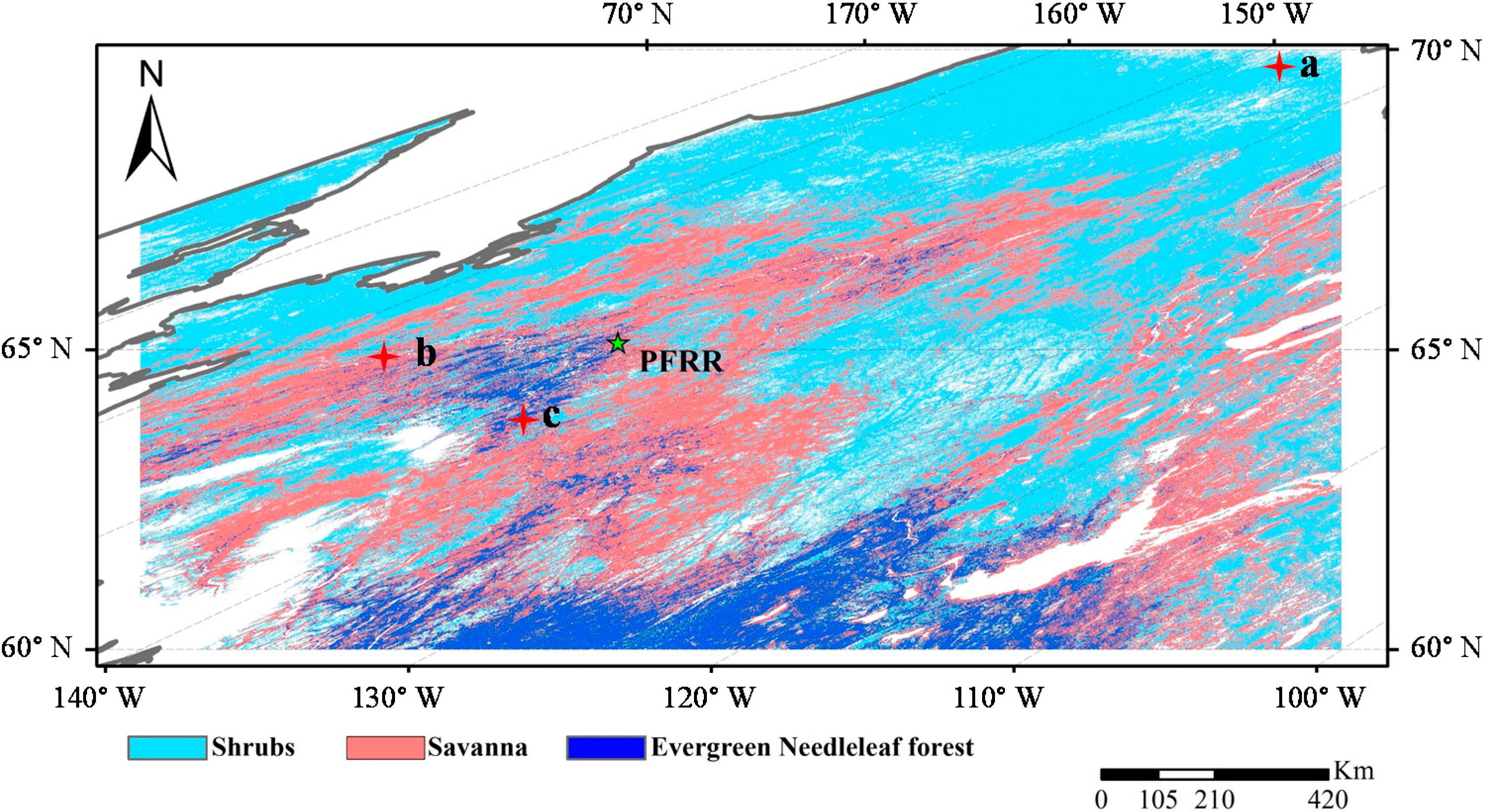
2.1. Study Area

The study area covers the main forest areas in Alaska and a small part of the Canadian forest (Figure 1), which together constitute two tiles of MODIS images (h11v02 and h12v02). The majority of the area is covered with evergreen needleleaf forest (Picea spp.), and the dominant species (98% of the overstory) is Black spruce (Picea mariana). Thus, the leaf area index of overstory canopy (LAIo) shows weak seasonality throughout the growing season [23]. The understory of the forests is covered with the mixtures of mosses, lichens, short herbaceous species, and dwarf shrubs according to field investigations [24].

Figure 1. Demonstration of the study area and land-cover types derived from MODIS data. PFRR denotes our investigation site, Poker Flat Research Range, and a, b, and c indicate the locations of pixels selected as examples of shrubs, savanna, and evergreen needleleaf forest, respectively (see Section 4.2 for details).

Figure 1. Demonstration of the study area and land-cover types derived from MODIS data. PFRR denotes our investigation site, Poker Flat Research Range, and a, b, and c indicate the locations of pixels selected as examples of shrubs, savanna, and evergreen needleleaf forest, respectively (see Section 4.2 for details).

According to the MODIS global Land Cover product (MOD12Q1 Collection 5, layer 3 for MODIS LAI/FPAR algorithm [25]), three vegetation types occur in our study area: shrubs, savanna, and evergreen needleleaf forest (Figure 1). In this classification scheme, needleleaf forest is defined as land dominated by trees with a percent canopy cover >60% and height exceeding 2 m. In contrast, the definition of shrub is land with woody vegetation less than 2 m tall and canopy cover >60% (closed shrub) or with woody vegetation less than 2 m tall and canopy cover ranging from 10% to 60% (open shrub). Savanna is defined as land with canopy cover ranging from 10% to 30% and height exceeding 2 m. Thus, most of the black spruce forest with relatively low canopy density in our study area is classified as shrub or savanna (Figure 1).

2.2. In Situ Data

Field investigations were carried out at the Poker Flat Research Range (PFRR, 65°07′N, 147°30′W), located 50 km from Fairbanks, Alaska, USA (Figure 1) during 14–17 July 2013. We measured reflectance spectra of understory at different locations using an ASD FieldSpec 4 spectral radiometer (ASD, Inc., Boulder, CO, US) at a 1-nm interval in the range of 350–2500 nm. We used halogen light (rather than natural sunlight) because the light environment at the understory level is not homogeneous. To avoid the influence of the overstory canopy on the measurement of understory reflectance, the ambient canopies were covered by black curtains, which shut out over 99% of the natural light. Then, the halogen light incident angle was set as 45°, and the fiber probe of the FieldSpec was positioned about 50 cm above the ground and set at 0° (nadir view). The integration time was optimized before each measurement over the reference panel. Measurements were taken at four plots covered with northern reindeer lichen, tussock, blueberry, and combinations of these. In total, reflectance spectra for 73 points were collected. All measurements were done in the same way. Figure 2 shows the reflectance spectra of forest understory collected in this study. Values shorter than 400 nm and longer than 2400 nm are not included due to instrument noise. High variability in the spectra due to the noticeably distinct land-cover properties can be observed. The spectra with high reflectance in the range of 800–1200 nm represent tussock, while the low spectra represent lichen.

Figure 2. Understory reflectance spectra collected at Poker Flat Research Range (PFRR), Alaska (N is the number of collected spectra.)

Figure 2. Understory reflectance spectra collected at Poker Flat Research Range (PFRR), Alaska (N is the number of collected spectra.)

2.3. MODIS Data

We used the MODIS BRDF/Albedo Product (MCD43A1, version 5, [26,27]) to reconstruct the bidirectional reflectance factor (BRF) in this study. The MCD43A1 provides the weighting parameters associated with the RossThick–LiSparse BRDF model that describes the reflectance anisotropy at 500-m resolution. The BRDF parameters are produced every eight days with 16 days of acquisition using both Terra and Aqua data [27].

MODIS data employed in this study were acquired for two tiles, namely h11v02 and h12v02, and day of year (DOY) values ranging from 145 to 257 (25 May to 14 September) during 2010–2013. During these periods, almost no snow cover existed in the study area. We downloaded all the MCD43A1 data and associated data quality (MCD43A2) from the Data Pool of Land Process Distributed Active Archive Center (LPDAAC). The MODIS land-cover products (MCD12Q1) during 2010–2012 were also downloaded from the same source (the data for 2013 were still not available) and were used for algorithm development.

2.4. Simulation Data Set

To validate the performance of the proposed method, we performed a radiative transfer simulation using the Forest Light Environment Simulator (FLiES, [28]). In this simulation, a typical heterogeneous black spruce landscape established by Kobayashi et al. [23] was used, specifically, 30 × 30-m² plot with stand density of 3978 trees∙ha⁻¹ (358 trees in the 30 × 30-m² plot). The average tree height and diameter at breast height (DBH) were 2.4 ± 1.1 m and 1.2 ± 0.079 cm, respectively. The crown diameters of all trees in the plot were determined through an empirical estimation equation based on DBH (i.e., crown diameter [m] = 0.044 DBH + 0.66, r² = 0.23, p < 0.01). The forest stand is composed of three layers: tree canopy, grass, and floor layers. The LAI for the tree canopy and the grass layer are denoted as LAIo (overstory) and LAIu (understory), respectively. The term “understory layer” here refers to the combination of the grass and floor layers. The LAIo changed from 0 to 2.0 at an interval of 0.1, and the LAIu varied from 0 to 2.5 at the same interval. Because we could not measure the bihemispherical reflectance and transmittance of the needle trees in this study, we instead used the bihemispherical reflectance and transmittance values of black spruce needle, which is the dominant species in our study area, reported by Hall et al. [29]. We also used the bihemispherical reflectance and transmittance values of grass reported by Myneni et al. [30], which are used for the MODIS global LAI product. Table 1 summarizes the optical parameters used in the simulation, where “floor reflectance” is the average reflectance of the non-vegetation objects collected in field investigations. Eight combinations of the solar-view angles were used: SZ = 45°, VZ = 0°, 10°, 20°, 30°, and RA = 40°, 140°. The BRF in red and near-infrared (NIR) bands for these angles were calculated from the FLiES.

Table 1. Optical properties used in the radiative transfer simulation.

	Needle Reflectance 1	Needle Transmittance 1	Grass Reflectance 2	Grass Transmittance 2	Stem Reflectance	Floor Reflectance
Red	0.074	0.023	0.116	0.112	0.051	0.079
NIR	0.466	0.387	0.427	0.479	0.091	0.225

¹ Needle reflectance and transmittance data are from Hall et al. [29]. ² Grass reflectance and transmittance data are from Myneni et al. [30].

Table 1. Optical properties used in the radiative transfer simulation.

	Needle Reflectance 1	Needle Transmittance 1	Grass Reflectance 2	Grass Transmittance 2	Stem Reflectance	Floor Reflectance
Red	0.074	0.023	0.116	0.112	0.051	0.079
NIR	0.466	0.387	0.427	0.479	0.091	0.225

¹ Needle reflectance and transmittance data are from Hall et al. [29]. ² Grass reflectance and transmittance data are from Myneni et al. [30].

3. Development of a New Method for Retrieving NDVIu

3.1. Theory

Conceptually, the reflectance of forest stands derives from two components: tree canopy and forest understory [31]. The term understory in this study refers to all the materials below forest canopies, such as grass, lichen, moss, and mixtures of these. If we imagine a decrease in the overstory LAI (LAIo) for a stand with a fixed understory, then the satellite-derived NDVI would be increasingly influenced by the understory. The NDVI values would decrease corresponding to the exposure of understory, as the tree canopy usually shows strong absorption in the red band but strong scattering in the NIR band. When LAIo decreases to zero, the corresponding NDVI value could simply be regarded as that of the understory [11]. This is apparently an idealized case because pixels with “zero-LAIo” usually do not exist in most of the forested areas. Even if they do exist, it is very hard (or impossible) to identify such pixels without additional prior information about the stand properties.

Alternatively, a linear extrapolation approach is developed in this study to derive NDVI values for a pixel with zero LAIo (i.e., NDVIu). In this method, we first identify a 5 × 5 window with the target pixel at the central position (Figure 3). See the Discussion in Section 5.2 for details regarding the determination of the window size. Within this window area, we make the following assumptions about the pixels classified as the same biome types: (1) the composition of the understory is identical across pixels; (2) the canopies’ optical and structural parameters other than LAIo, such as tree height, crown depth, leaf angle distribution, leaf reflectance and transmittance, and stem reflectance, are identical across pixels; and (3) the LAIo values are variable among pixels. These assumptions can possibly be satisfied in natural forests. Accordingly, the LAIo is the sole source for the variability of NDVI among the pixels for a specified solar-view angle.

Figure 3. Conceptual demonstration of the method for retrieving NDVIu (5 × 5 window with the center as target pixel; only the pixels with the same vegetation type as the target pixel are used for regression analysis. Grids with different format indicate different land-cover categories).

Figure 3. Conceptual demonstration of the method for retrieving NDVIu (5 × 5 window with the center as target pixel; only the pixels with the same vegetation type as the target pixel are used for regression analysis. Grids with different format indicate different land-cover categories).

Then, we performed regression analysis among the NDVI values of the pixels corresponding to different angles, which were reconstructed from MODIS BRDF product. Linear regression was performed with the nadir-view NDVI values as the independent variable and NDVI values corresponding to other bidirectional angles as dependent factors. Having the same canopy structure but variable LAIo would make the correlations significant.

Last, we determined the value of NDVIu according to a useful property of the stand: the angular variation in NDVI for a stand with LAIo = 0 (i.e., the forest understory) was smaller than that for a stand with none-zero LAIo. Therefore, the retrieved NDVIu is defined as the mean of NDVI values in which the regression lines have the smallest standard deviation. See the following section on implementation of the method.

It is worth noting that for a stand with LAIo = 0, stems and branches would scatter light and cast shadows on the understory layer, which might make the estimated NDVIu from our method different from the real understory NDVI. However, for the sparse forests, this difference should be negligible due to the rather low canopy coverage. Thus, we simply take the estimated NDVIu as real understory NDVI in this study.

3.2. Implementation Steps

The retrieval of NDVIu from MODIS BRDF data is implemented according to the following steps:

Step 1 was to reconstruct the BRF values. Eight BRF values for the red and near-infrared (NIR) bands were reconstructed, corresponding to the combinations of (1) solar zenith angle (SZ) = 45°; (2) view zenith angle (VZ) = 0°, 10°, 20°, and 30°; and (3) relative azimuth angle (RA) = 40°, 140°. We determined these angles to avoid very large zenith angles and the hot spot direction (the RA is little off from the principal plane). The NDVI values for the eight angle combinations were then calculated accordingly.

Step 2 was to perform the regression analysis. For the 5 × 5 window with the target pixel at the central position (Figure 3), only the pixels classified as the same vegetation type as the target pixel were selected for the linear regression. Using the nadir-view NDVI as the independent factor (x-axis), we can obtain seven regression equations as follows:

NDVI_i = a_i × NDVI₀ + b_i

(1)

where NDVI₀ denotes the NDVI values for a nadir-view position (SZ = 45°, VZ = 0° and RA = 140°), and NDVI_i (i = 1, 2, …, 7) denotes the NDVI values for other seven solar-view angles.

Step 3 was to search the position at which the regressed NDVI_i has the lowest variation. Let the NDVI₀ change from 0 to 1.0 at an interval of 0.01. We calculated the standard deviation (SD) among the seven regression equations (shown as Equation (1)) corresponding to each value of NDVI₀. Consequently, we obtained the value of NDVI₀ that corresponds to the lowest SD (denoted as NDVI_0,S).

Step 4 was to retrieve NDVIu. NDVIu is calculated as the average of the regression NDVI values with the lowest bidirectional variability:

$$\mathrm{N}\mathrm{D}\mathrm{V}\mathrm{I}\mathrm{u}=\frac{{\displaystyle \sum _{i=1}^N(a_{ \mathrm{i}}\times {\mathrm{N}\mathrm{D}\mathrm{V}\mathrm{I}}_{0, \mathrm{S}}+b_{\mathrm{i}})}}{N}$$

(2)

in which N is the number of solar-view angles used in regression analysis (N = 7 in this study).

4. Results

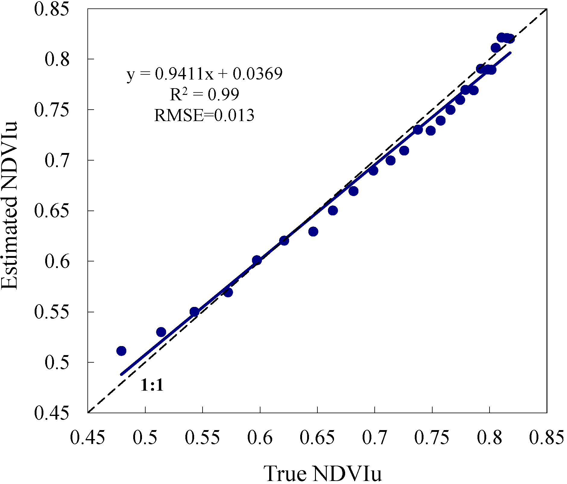
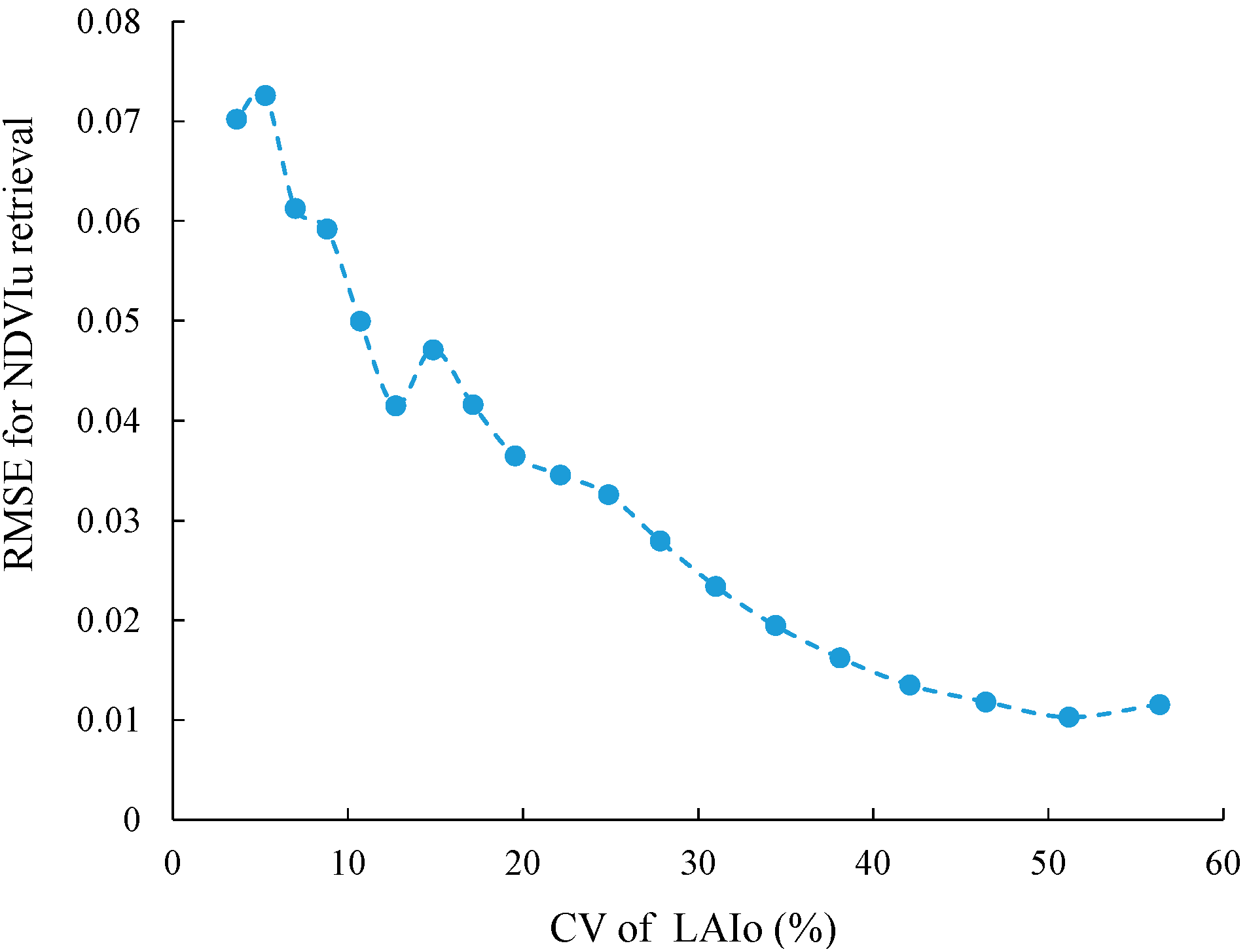
4.1. Results for Simulation Data Set

The proposed method was first applied to the simulation data set. Figure 4 shows an example of the scatterplot between the nadir-view NDVI and the NDVI values for seven other angles; for all samples, LAIu = 0.5. Only the simulation samples with LAIo between 0.5 and 2.0 were used for the regression analysis. This is used to mimic the situation we might encounter in the study area: the canopy LAI varies in the range of 0.5 to 2.0 within a 5 × 5 window. The correlations were all significant, with the R² values higher than 0.99. The variation in the seven regression lines decreased from the higher tail of the NDVI values, then increased beyond the convergence point of the regression lines. This point is the position at which the SD of the seven regression lines has the smallest value (denoted by a red dashed line in Figure 4). Then, the estimation of NDVIu is calculated as the average of the seven regression lines corresponding to the position at which the SD is smallest. The cases corresponding to other levels of LAIu have similar outcomes. These results imply that the rationale of our proposed method is reasonable.

Figure 4. An example of scatterplots of the relationship between the nadir-view NDVI and NDVI for other bidirectional angles from the simulation data set.

Figure 4. An example of scatterplots of the relationship between the nadir-view NDVI and NDVI for other bidirectional angles from the simulation data set.

Moreover, Figure 5 shows the comparison between the true NDVIu (i.e., the NDVI for the stands with LAIo = 0) and the retrieved NDVIu by our proposed method. For all the samples, the input values of LAIu in the FLiES simulation ranged from 0 to 2.5 with an interval of 0.1. Thus, there are 26 points in total. It can be seen that the estimated values are highly consistent with the true values, with R² and RMSE of 0.99 and 0.013 and the slope and intercept very close to “1” and “0”, respectively. This is an idealized case without contamination caused by measurement errors, and the simulated conditions totally satisfy the basic assumptions of the proposed method. The high accuracy of the retrieval results demonstrates that the proposed method is theoretically reasonable.

An important prerequisite of our method is that the LAIo of samples used for regression analysis have a reasonable dynamic range. By using the simulation data set, we tested the influence of the dynamic range of LAIo on the accuracy of NDVIu retrieval. We used groups of samples with different values for the coefficient of variation (CV; defined as the ratio of the standard deviation to the average) for LAIo to retrieve NDVIu. The corresponding root-mean-square-error (RMSE) for each level of CV was also calculated (Figure 6). As predicted, the RMSE decreases when the CV of LAIo increases. When CV is beyond 40%, the RMSE becomes stable and lower than 0.015.

Figure 5. Comparison between true and retrieved NDVIu values for cases with LAIu ranging from 0 to 2.5.

Figure 5. Comparison between true and retrieved NDVIu values for cases with LAIu ranging from 0 to 2.5.

Figure 6. RSME for NDVIu retrieval corresponding to different levels of coefficient of variation (CV) for LAIo.

Figure 6. RSME for NDVIu retrieval corresponding to different levels of coefficient of variation (CV) for LAIo.

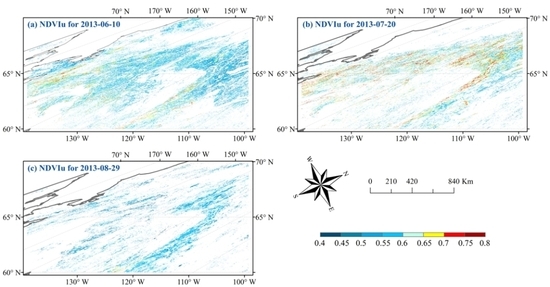
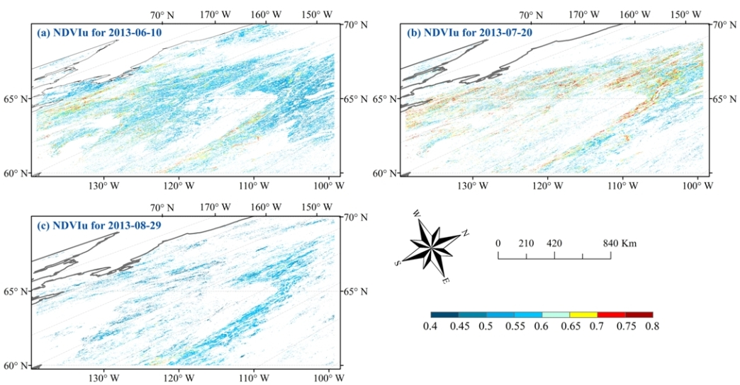
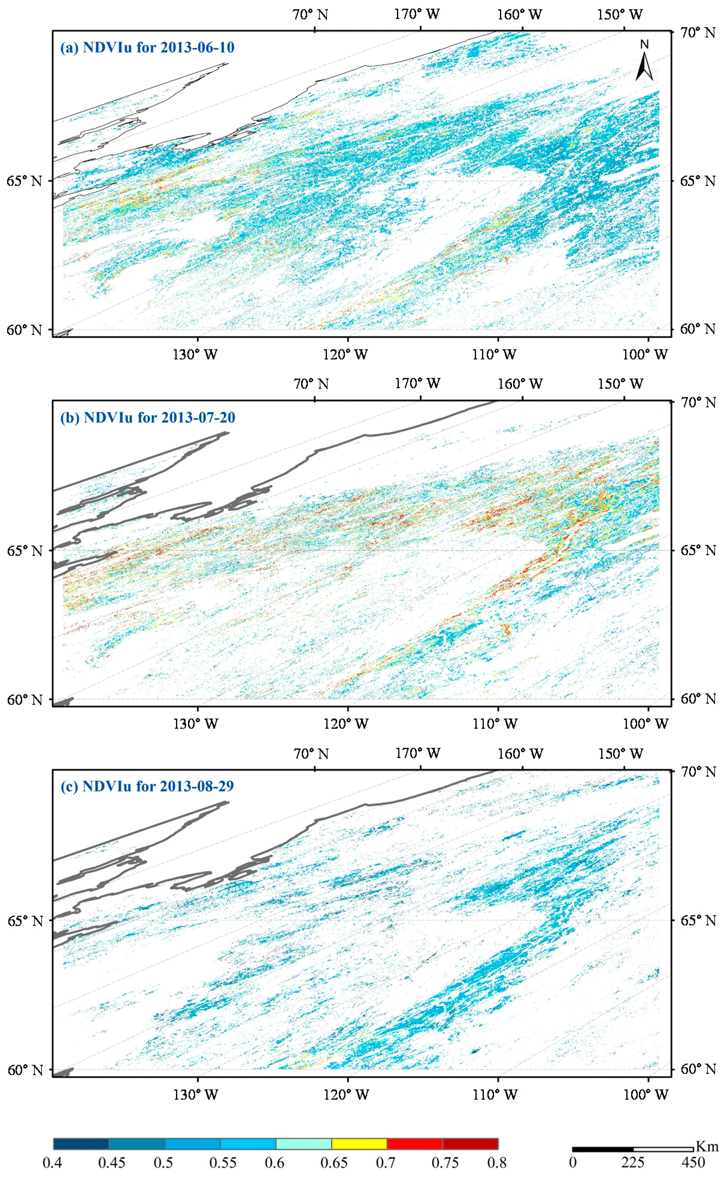
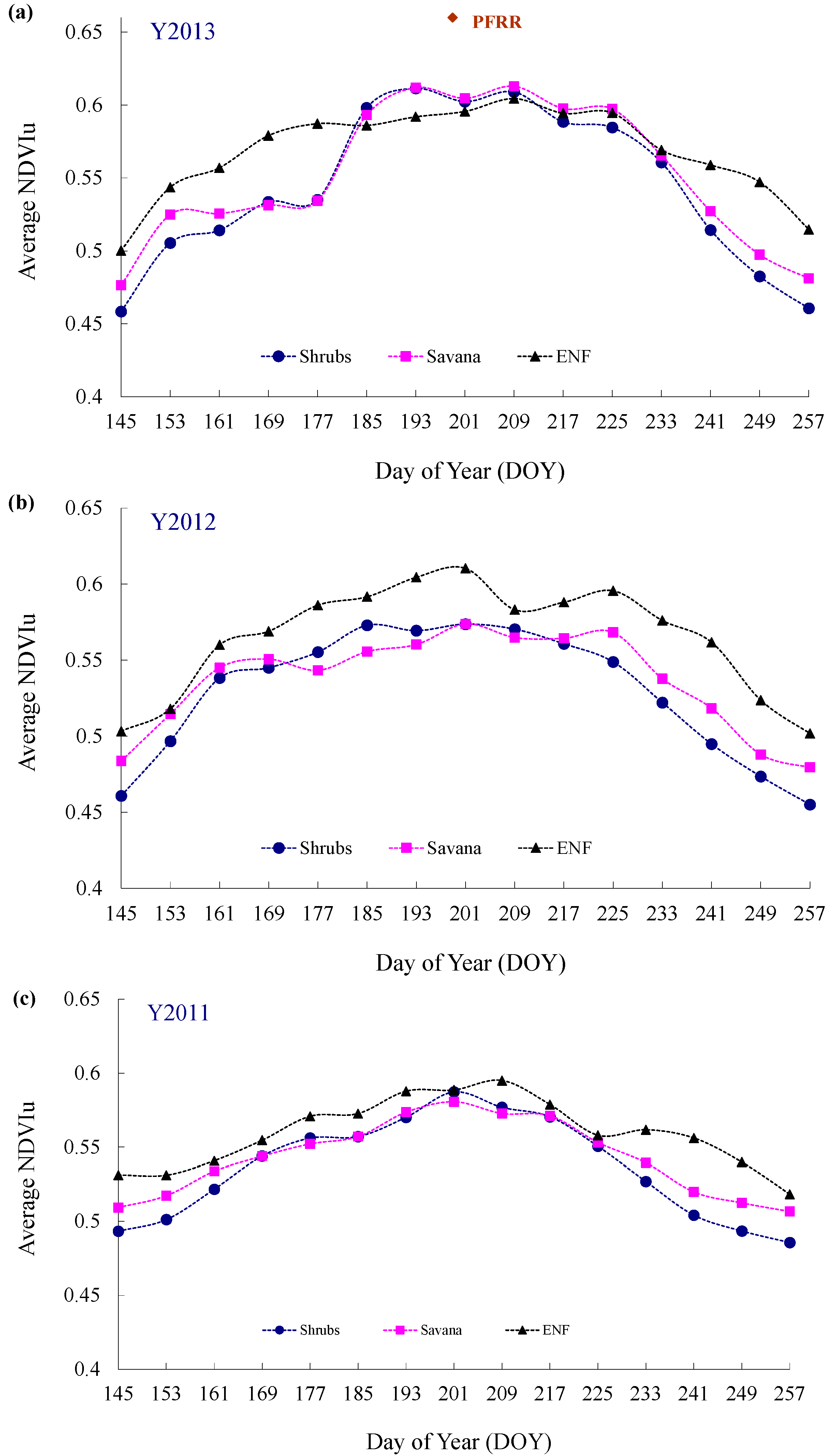
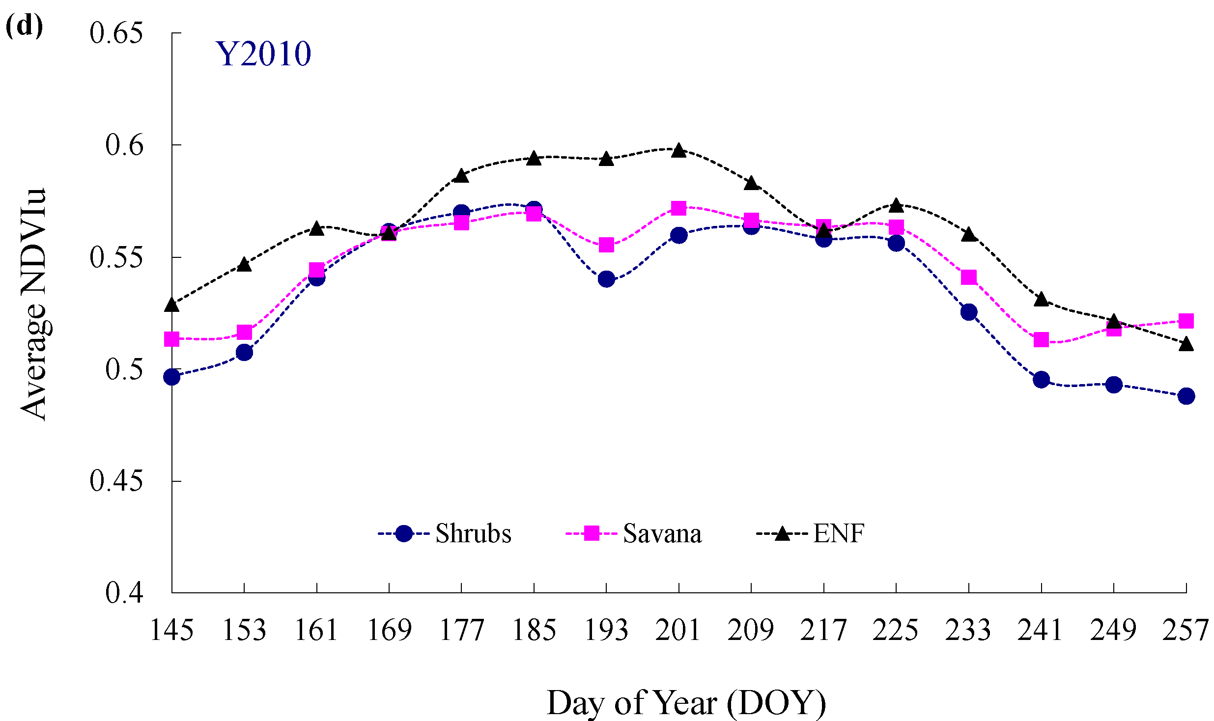
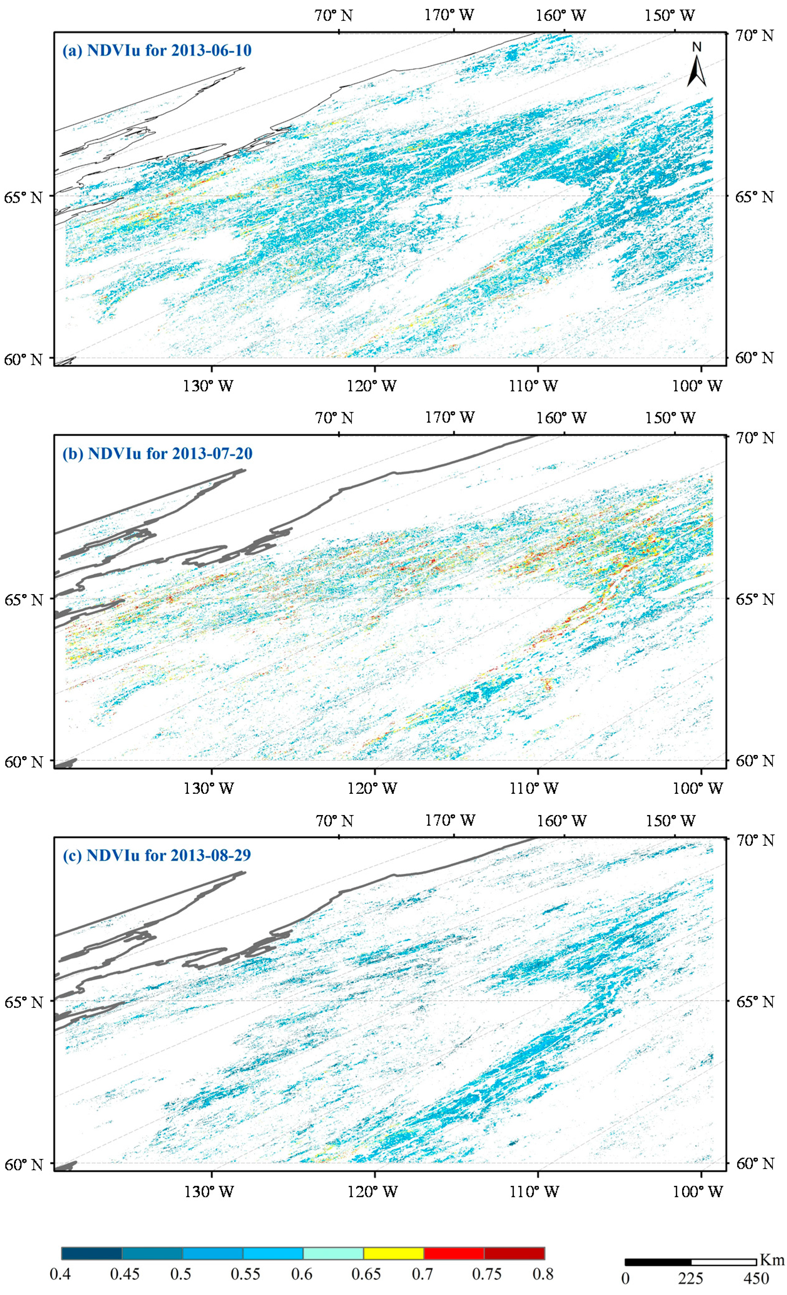
4.2. Results of MODIS Data

The proposed method was then applied to the MODIS BRDF data for 2010 to 2013 with DOY of 145 to 257, periods during which almost no snow cover was observed in the study area. Considering the possible noise in the BRDF product and the complicated natural situations, we used the following quality filtering criteria to screen the retrieval results:

(1)

The number of pixels used for regression analysis should be greater than nine.

(2)

All the R² values for the linear regression should be higher than 0.7.

(3)

The retrieval values of NDVIu should not be larger than the minimum NDVI within the 5 × 5 window.

Using these criteria, it is not surprising that we could not retrieve NDVIu for each pixel. The pixels not satisfying these criteria were discarded and marked as “no retrieval”.

Figure 7. Examples of scatterplots of the relationship between the nadir-view NDVI and NDVI for other bidirectional angles from the MODIS BRDF data for three different biomes: (a) shrubs; (b) savanna; and (c) evergreen needleleaf forest (ENF).

Figure 7. Examples of scatterplots of the relationship between the nadir-view NDVI and NDVI for other bidirectional angles from the MODIS BRDF data for three different biomes: (a) shrubs; (b) savanna; and (c) evergreen needleleaf forest (ENF).

Figure 7 shows three examples of the scatterplots between the nadir-view NDVI and the NDVI values for the other seven angle combinations. These examples were randomly selected from the valid retrievals in the DOY 201 image of 2013 corresponding to three biome types: savanna, shrubs, and evergreen needleleaf forest (ENF), respectively. The locations of the examples are shown as a, b, and c in Figure 1. The scatterplots for MODIS data show similar characteristics to those of the simulation data set (see Figure 4 for comparison). That is, the variation in the seven regression lines decreased from the higher tail of the NDVI values and then increased beyond a particular position, indicated by red dashed lines in Figure 7a–c. The retrieval of NDVIu was calculated as the average of the seven regression lines at the marked position. The results demonstrate that the proposed method is applicable to the MODIS BRDF product for our study area.

Figure 8. Three examples of the spatial distribution of retrieved understory NDVI (NDVIu) on (a) 10 June; (b) 20 July; and (c) 29 August 2013, using the 5 × 5 window.

Figure 8. Three examples of the spatial distribution of retrieved understory NDVI (NDVIu) on (a) 10 June; (b) 20 July; and (c) 29 August 2013, using the 5 × 5 window.

Figure 8 shows three examples of the spatial distribution of NDVIu retrievals for 10 June, 20 July, and 29 August 2013, respectively. As stated above, we did not obtain valid retrieval of NDVIu for each pixel due to the use of quality-filtering criteria. The percentages of pixels with valid NDVIu retrievals were 26.16%, 15.61%, and 10.24% for the three periods, respectively. The retrieved values of NDVIu showed remarkable seasonal variability. In late spring (10 June, Figure 8a), most of the NDVIu values were 0.45–0.55, whereas in mid-summer (20 July, Figure 8b), the NDVIu increased to 0.6–0.75. Then, at the end of summer (29 August, Figure 8c), the NDVIu decreased to 0.45–0.55.

Figure 9. Time series of the average NDVIu for different biome types (shrubs, savanna, and evergreen needleleaf forest) in years (a) 2013; (b) 2012; (c) 2011; and (d) 2010 (The average of in situ measured understory NDVI on 17 July 2013, at PFRR is also shown in (a) for comparison).

Figure 9. Time series of the average NDVIu for different biome types (shrubs, savanna, and evergreen needleleaf forest) in years (a) 2013; (b) 2012; (c) 2011; and (d) 2010 (The average of in situ measured understory NDVI on 17 July 2013, at PFRR is also shown in (a) for comparison).

Furthermore, we calculated the average NDVIu for the biome types shrubs, savanna, and ENF for DOY from 145 to 257 in 2010–2013 (Figure 9). The average in situ understory NDVI measured at PFRR, whose biome type in July 2013 was savanna, according to IGBP land-cover biome classification, is also shown in Figure 9a. The in situ NDVIu average was 0.66 with an SD of 0.12, comparable to the MODIS retrieval closest to the investigation date for savanna, whose average was 0.61, with an SD of 0.10. It should be noted that the BRDF product did not yield a valid NDVIu retrieval value for the pixel covering PFRR mainly because of the low data quality. Therefore, we cannot perform a standard comparison of the in situ measurement and the retrieval from satellite data. However, the small discrepancy (0.66 ± 0.12 vs. 0.61 ± 0.10) suggested that the retrieved NDVIu yielded an acceptable range for the NDVI values for the forest understory. Moreover, the times series of the retrieved NDVIu for each biome in each year showed an increasing trend from Spring to Summer, and then a decreasing trend from Summer to Autumn (Figure 9). This is completely consistent with the phenology pattern of grass within the study area.

5. Discussion

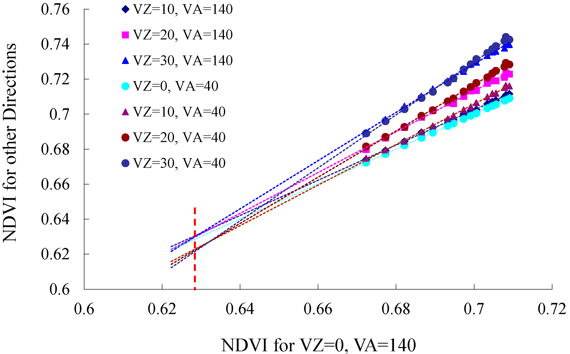
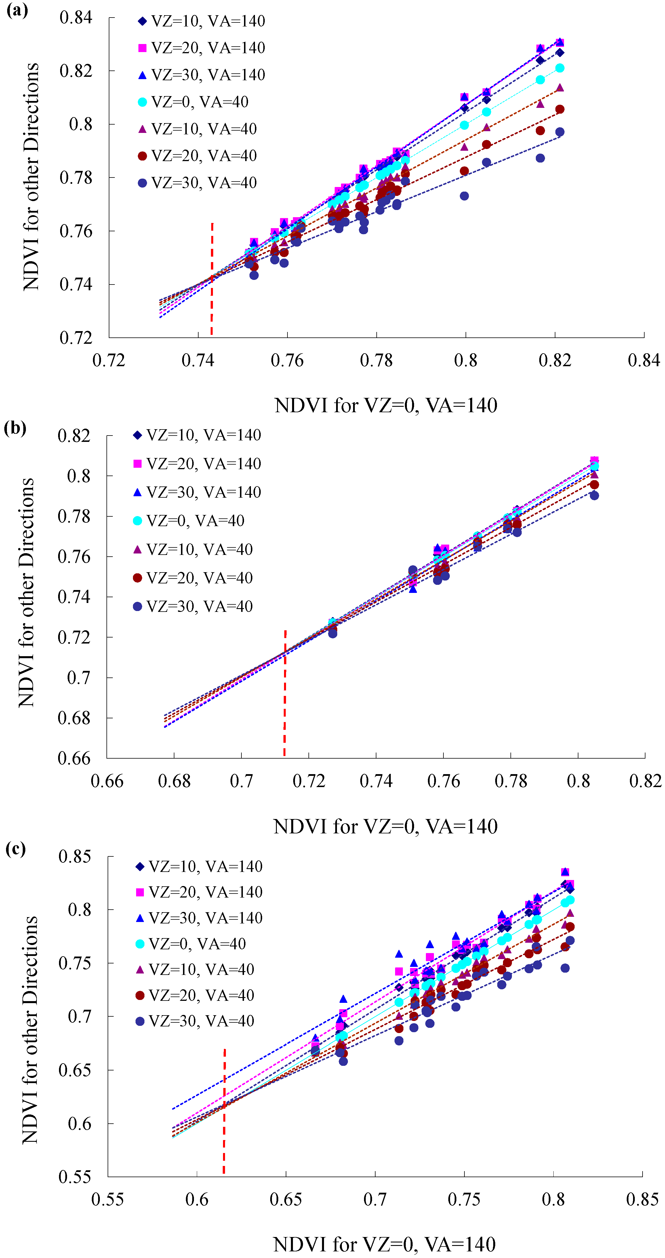
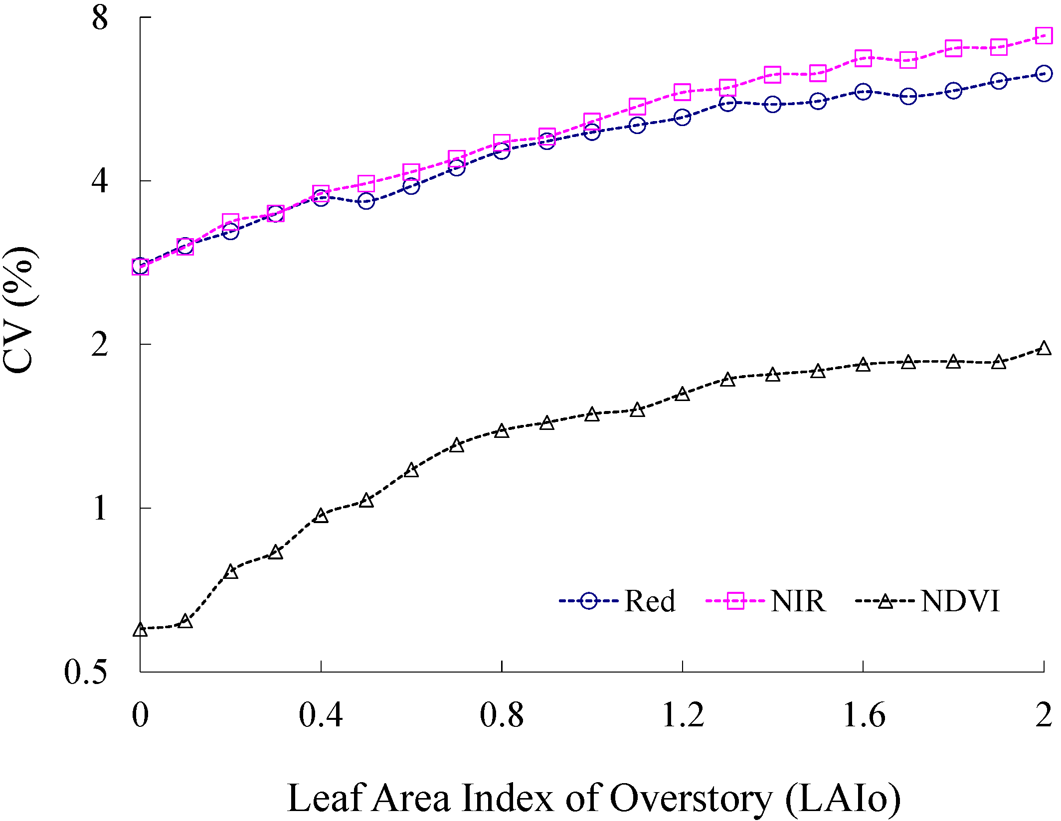
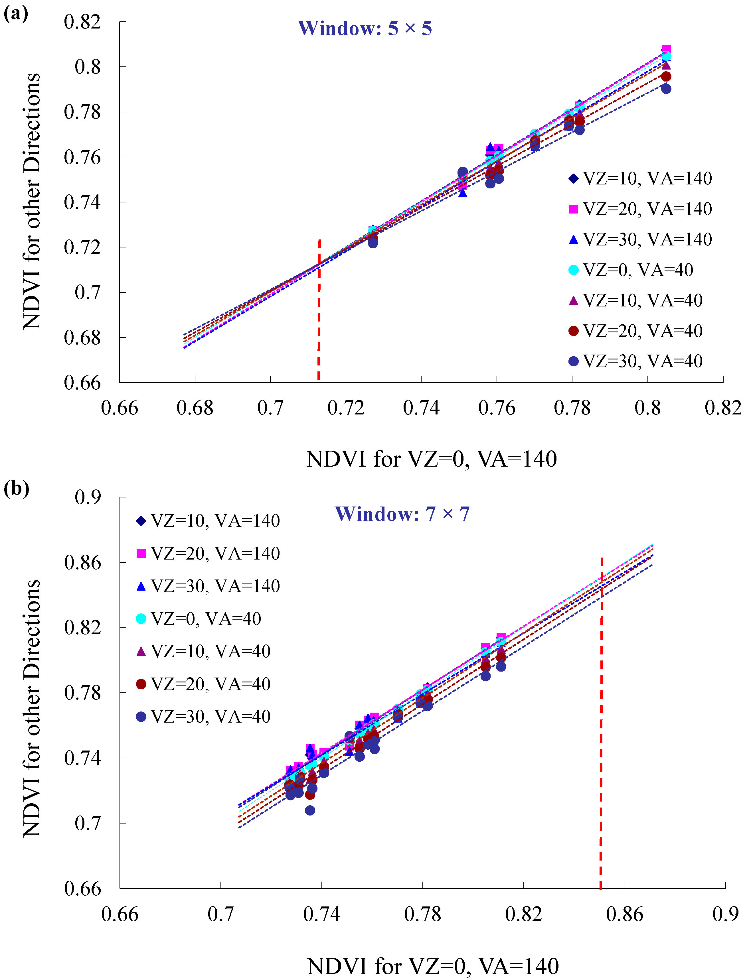
5.1. Angular Variations in BRF for the Stands with Variable LAIo Values

In our proposed method, the NDVIu is estimated according the property of a forest stand that the angular variation in NDVI for a stand with LAIo = 0 (i.e., NDVIu) is smaller than that of a stand with non-zero LAIo. According to the theory of the four-scale geo-optical model [19], the reflectance of a forest stand can be calculated as the weighted sum of four components: the sunlit and shaded overstory canopy and sunlit and shaded understory layer. Angular variability is caused by the different contributions of the four components to stand reflectance. For the case of the understory layer only with no overstory, there is only one component, namely, sunlit understory; in contrast, in the case of understory layer with an overstory canopy, four components exist, as mentioned previously. Because the understory and overstory usually show distinct BRDF properties, it is natural to consider that the case of understory with overstory has larger angular variability than the case with only understory.

To validate this property, we utilized a simulation data set, as delineated in Section 4.1. The CV of BRF at red and NIR bands and NDVI corresponding to the eight solar-view angles were calculated (Figure 10). It can be seen that all of the CV curves for the two bands and the corresponding NDVI show an increasing trend when LAIo increases. In other words, the stand with LAIo = 0 has the smallest angular variation among the stands having LAIo in the range 0–2.0. Consequently, we may consider that the NDVI values also have the smallest variation when the stand has LAIo = 0. It should be noted that all the demonstrated samples were had LAIu values >0.5; therefore, the CV corresponding to LAIo = 0 is not zero.

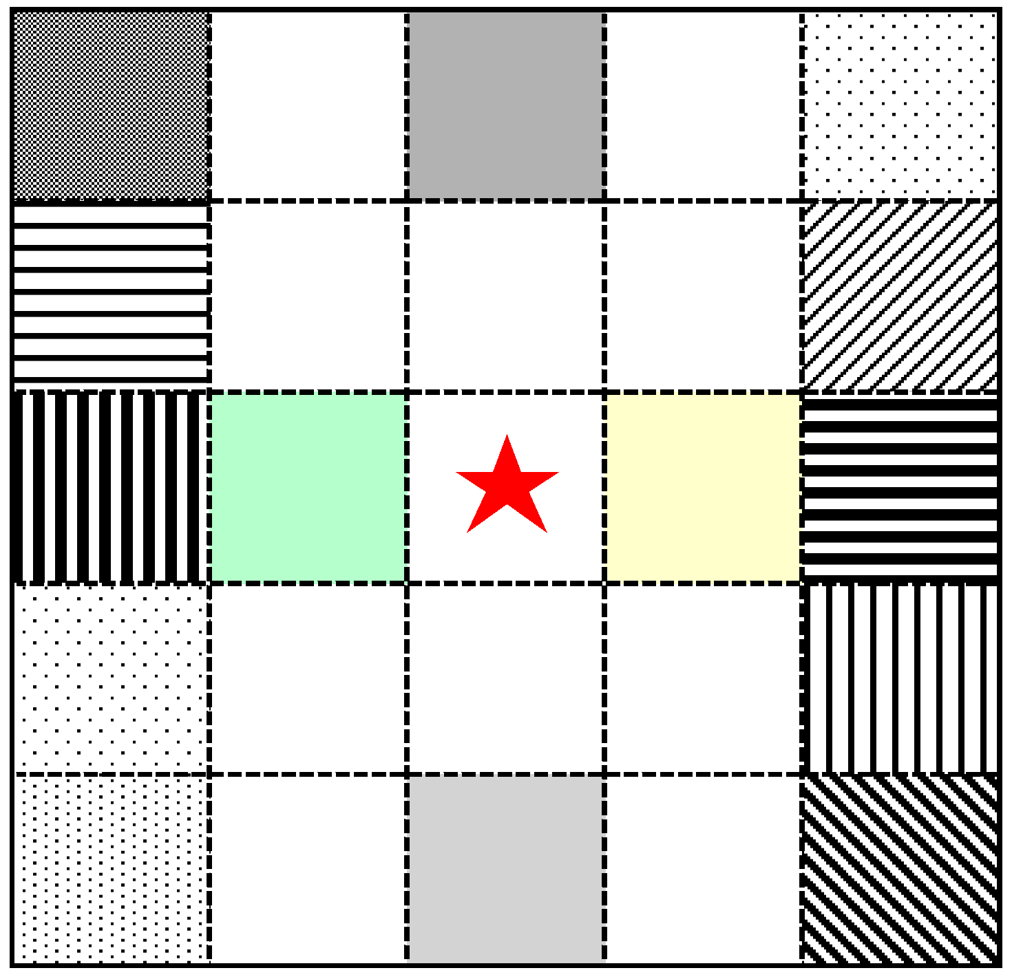
5.2. How to Determine the Window Size

A practical problem in applying the proposed method is determining which window size should be used to perform the regression analysis. Selection of the window size is actually a trade-off between the number of pixels that are valid for regression and the homogeneity of the understory layer. On the one hand, the window size should be large enough to guarantee that enough pixels are available for regression analysis and that the variation in overstory LAI has an adequate dynamic range. On the other hand, the window size should not be too large to make the properties of the understory layer inhomogeneous within the window.

Figure 10. Coefficient of variation (CV) in BRF at red and NIR bands, and NDVI for the stands with different values of LAIo.

Figure 10. Coefficient of variation (CV) in BRF at red and NIR bands, and NDVI for the stands with different values of LAIo.

In this study, the window size is determined through a trial-and-error approach. We manually tested the effect of window size on the retrieval of NDVIu, including window sizes of 3 × 3, 5 × 5, and 7 × 7. Figure 11 shows an example, based on the case shown in Figure 7b, of how the window size affects the retrieval of NDVIu. For the 3 × 3 window, only five pixels were valid for regression analysis. Thus, it was discarded. The 5 × 5 window demonstrated acceptable performance (Figure 11a). For the case of 7 × 7 window, as shown in Figure 11b, the position at which the seven regression lines have the smallest SD is larger than the maximum NDVI within the window, which violates the premise that the stand with higher LAIo should have higher NDVI values. Consequently, we cannot obtain valid retrieval of NDVIu for this case.

Figure 11. An example of NDVIu retrieval using window sizes of (a) 5 × 5 and (b) 7 × 7. (The 3 × 3 window size cannot provide satisfactory samples for regression analysis; thus, is not shown here).

Figure 11. An example of NDVIu retrieval using window sizes of (a) 5 × 5 and (b) 7 × 7. (The 3 × 3 window size cannot provide satisfactory samples for regression analysis; thus, is not shown here).

By using the 7 × 7 window, the spatial distribution of retrieved NDVIu from MODIS BRDF data was also derived for 10 June 20 July and 29 August 2013 (Figure 12). It can be seen that the results yielded similar regional patterns to those derived from the 5 × 5 window, as shown in Figure 8. However, the percentage of valid retrievals obtained using a 7 × 7 window were lower than those obtained using a 5 × 5 window (23.29%, 13.64%, and 7.58% vs. 26.16%, 15.61%, and 10.24% for the three dates, respectively). The use of s 7 × 7 window yielded fewer valid retrievals of NDVIu than did the 5 × 5 window for other dates of MODIS images as well. Consequently, the 5 × 5 window was used in this study. For the MODIS BRDF product, it corresponds to a scale of 2.5 × 2.5 km. It should be noted that the window size was empirically determined in this study. For other study areas, a more appropriate window size should be decided prior to the retrieval of NDVIu.

Figure 12. Spatial distribution of retrieved understory NDVI (NDVIu) on (a) 10 June; (b) 20 July; and (c) 29 August 2013, using the 7 × 7 window.

Figure 12. Spatial distribution of retrieved understory NDVI (NDVIu) on (a) 10 June; (b) 20 July; and (c) 29 August 2013, using the 7 × 7 window.

5.3. Toward Practical Applications of the Retrieved NDVIu

The greatest merit of the proposed method is that it is very easy to implement. That is, no complicated physical models are required, nor are any look-up tables. Although the proposed method is semi-empirical, it relies not only on data analysis but also on the theoretical consideration of the radiative transfer model. Nevertheless, it is proposed based on several basic assumptions (see Section 3.1 for details). For example, we assume that the understory for a pixel (area of 0.25 km²) is similar to its two ambient pixels (i.e., 5 × 5 pixel window). This assumption may not be satisfied for some forests. Therefore, we cannot expect that our method can be applicable everywhere. Consequently, we cannot derive the retrieval of NDVIu in some cases. Improving the retrieval rate of NDVIu will be carried out in future works. However, the present approach can be regarded as an alternative to the data bank method for dealing with the background properties (e.g., [12,14]), and it provides a much larger number of samples than conventional in situ methods do by covering wide areas and long periods. It is also worth noting that the performance of the proposed method would be influenced by the accuracy of land-cover products. Use of more accurate land-cover data than MODIS products can possibly improve the estimation of NDVIu.

In sparse boreal forests, contribution of understory vegetation to carbon sources and sinks is not negligible [24,32]. Therefore, it is necessary to evaluate the amount of understory as well as overstory vegetation. The retrieved NDVIu can be directly related with the status of understory vegetation. On the other hand, the retrieved NDVIu can also be applied to improve the estimation of overstory LAI in the sparse boreal forests, as Miller et al. [11] pointed out that inclusion of the zero-LAI understory-derived indices significantly enhanced the correlation in the linear VI-LAI relationships. Ultimately, retrieval of NDVIu can benefit studies on carbon cycle modeling over the high-latitude areas by taking into consideration the different residence times for different vegetation components in forest ecosystems [33]. These issues will be addressed in future studies.

6. Conclusions

In this study, we proposed a simple semi-empirical method to understory Normalized Difference Vegetation Index (NDVIu) for sparse boreal forests from the MODerate resolution Imaging Spectroradiometer (MODIS) Bidirectional Reflectance Distribution Function (BRDF) data. The theory of the method is based on the fact that the bidirectional variation in NDVIu is smaller than that in canopy-level NDVI. To retrieve NDVIu for a certain target pixel, linear extrapolation was applied using pixels within a 5 × 5 target-pixel-centered window. The NDVI values were reconstructed from the MODIS BRDF data corresponding to eight different solar-view angles. NDVIu was estimated as the average of the NDVI values corresponding to the position in which the stand NDVI had the smallest angular variation. Validation by a noise-free simulation data set yielded high agreement between estimated and true NDVIu, with coefficient of determination (R²) and root-mean-square-error (RMSE) of 0.99 and 0.03, respectively. Using the MODIS BRDF data, we achieved an estimate of NDVIu close to the in situ measured value (0.61 vs. 0.66 for estimate and measurement, respectively) and reasonable seasonal patterns of NDVIu during 2010–2013. The retrieval of NDVIu can be used to improve the estimation of leaf area index (LAI) in sparsely vegetated areas, and also possibly be used to study the phenology of understory layer.

References

1. Chen, J.M.; Black, T.A. Defining leaf area index for non-flat leaves. Plant Cell Environ. 1992, 15, 421–429. [Google Scholar] [CrossRef]
2. Pinty, B.; Lavergne, T.; Kaminski, T.; Aussedat, O.; Giering, R.; Gobron, N.; Taberner, M.; Verstraete, M.M.; Voβbeck, M.; Widlowski, J.L. Partitioning the solar radiant fluxes in forest canopies in the presence of snow. J. Geophys. Res. 2008. [Google Scholar] [CrossRef]
3. Baret, F.; Hagolle, O.; Geiger, B.; Bicheron, P.; Miras, B.; Huc, M.; Berthelot, B.; Nino, F.; Weiss, M.; Samain, O.; et al. LAI, fAPAR and fCover CYCLOPES global products derived from VEGETATION Part 1: Principles of the algorithm. Remote Sens. Environ. 2007, 110, 275–286. [Google Scholar] [CrossRef] [Green Version]
4. Knyazikhin, Y.; Martonchik, J.V.; Myneni, R.B.; Diner, D.J.; Running, S.W. Synergistic algorithm for estimating vegetation canopy leaf area index and fraction of absorbed photosynthetically active radiation from MODIS and MISR data. J. Geophys. Res. 1998, 103, 32257–32275. [Google Scholar] [CrossRef]
5. Liu, Y.; Liu, R.; Chen, J.M. Retrospective retrieval of long-term consistent global leaf area index (1981–2011) from combined AVHRR and MODIS data. J. Geophys. Res. 2012. [Google Scholar] [CrossRef]
6. Fang, H.; Jiang, C.; Li, W.; Wei, S.; Baret, F.; Chen, J.M.; Garcia-Haro, J.; Liang, S.L.; Liu, R.; Myneni, R.B.; et al. Characterization and intercomparison of global moderate resolution leaf area index (LAI) products: Analysis of climatologies and theoretical uncertainties. J. Geophys. Res. 2013, 118, 529–548. [Google Scholar]
7. Chopping, M.; Su, L.; Rango, A.; Maxwell, C. Modelling the reflectance anisotropy of Chihuahuan Desert grass-shrub transition canopy soil complexes. Int. J. Remote Sens. 2004, 25, 2725–2745. [Google Scholar] [CrossRef]
8. Kuusk, A.; Nilson, T. A directional multispectral forest reflectance model. Remote Sens. Environ. 2000, 72, 244–252. [Google Scholar] [CrossRef]
9. Chopping, M.J.; Rango, A.; Havstad, K.M.; Schiebe, F.R.; Ritchie, J.C.; Schmugge, T.J.; French, A.N.; Su, L.; McKee, L.; Davis, M.R. Canopy attributes of desert grassland and transition communities derived from multiangular airborne imagery. Remote Sens. Environ. 2003, 85, 339–354. [Google Scholar] [CrossRef]
10. Dangel, S.; Verstraete, M.M.; Schopfer, J.; Kneubuehler, M.; Schaepman, M.; Itten, K.I. Toward a direct comparison of field and laboratory goniometer measurements. IEEE Trans. Geosci. Remote Sens. 2005, 43, 2666–2675. [Google Scholar] [CrossRef]
11. Miller, J.R.; White, H.P.; Chen, J.M.; Peddle, D.R.; McDermid, G.; Fournier, R.A.; Shepherd, P.; Rubinsterin, I.; Freemantel, J.; Soffer, R.; et al. Seasonal change in understory reflectance of boreal forest and influence on canopy vegetation indices. J. Geophys. Res. 1997, 102, 29475–29482. [Google Scholar] [CrossRef]
12. Peltoniemi, J.I.; Kaasalainen, S.; Näränen, J.; Rautiainen, M.; Stenberg, P.; Smolander, H.; Smolander, S.; Voipio, P. BRDF measurement of understory vegetation in pine forests: Dwarf shrubs, lichen, and moss. Remote Sens. Environ. 2005, 94, 343–354. [Google Scholar] [CrossRef]
13. Suzuki, R.; Kobayashi, H.; Delbart, N.; Asanuma, J.; Hiyama, T. NDVI responses to the forest canopy and floor from spring to summer observed by airborne spectrometer in eastern Siberia. Remote Sens. Environ. 2011, 115, 3615–3624. [Google Scholar] [CrossRef]
14. Kuusk, A.; Lang, M.; Nilson, T. Simulation of the reflectance of ground vegetation in sub-boreal forests. Agric. For. Meteorol. 2004, 126, 33–46. [Google Scholar] [CrossRef]
15. Deng, F.; Chen, J.M.; Plummer, S.; Chen, M.; Pisek, J. Algorithm for global leaf area index retrieval using satellite imagery. IEEE Trans. Geosci. Remote Sens. 2006, 44, 2219–2229. [Google Scholar] [CrossRef]
16. Pisek, J.; Chen, J.M. Comparison and validation of MODIS and VEGETATION global LAI products over four BigFoot sites in North America. Remote Sens. Environ. 2007, 109, 81–94. [Google Scholar] [CrossRef]
17. Pisek, J.; Chen, J.M. Mapping forest background reflectivity over North America with Multi-angle Imaging SpectroRadiometer (MISR) data. Remote Sens. Environ. 2009, 113, 2412–2423. [Google Scholar] [CrossRef]
18. Canisius, F.; Chen, J. Retrieving forest background reflectance in a boreal region from Multi-angle Imaging SpectroRadiometer (MISR) data. Remote Sens. Environ. 2007, 107, 312–321. [Google Scholar] [CrossRef]
19. Chen, J.M.; Leblanc, S.G. A four-scale bidirectional reflectance model based on canopy architecture. IEEE Trans. Geosci. Remote Sens. 1997, 35, 1316–1337. [Google Scholar] [CrossRef]
20. Leblanc, S.G.; Bicheron, P.; Chen, J.M.; Leroy, M.; Cihlar, J. Investigation of directional reflectance in boreal forests with an improved 4-Scalemodel and airborne POLDER data. IEEE Trans. Geosci. Remote Sens. 1999, 37, 1396–1414. [Google Scholar] [CrossRef]
21. Pisek, J.; Chen, J.M.; Miller, J.R.; Freemantle, J.R.; Peloniemi, J.I.; Simic, A. Mapping forest background reflectance in a boreal region using multiangle compact airborne spectrographic imager data. IEEE Trans. Geosci. Remote Sens. 2010, 48, 499–510. [Google Scholar]
22. Pisek, J.; Rautiainen, M.; Heiskanen, J.; Mõttus, M. Retrieval of seasonal dynamics of forest understory reflectance in a Northern European boreal forest from MODIS BRDF data. Remote Sens. Environ. 2012, 117, 464–468. [Google Scholar] [CrossRef]
23. Kobayashi, H.; Suzuki, R.; Nagai, S.; Nakai, T.; Kim, Y. Spatial scale and landscape heterogeneity effects on FAPAR in an open-canopy black spruce forest in interior Alaska. IEEE Geosci. Remote Sens. Letters 2013, 11, 564–568. [Google Scholar] [CrossRef]
24. Kushida, K.; Kim, Y.; Tanaka, N.; Fukuda, M. Remote sensing of net ecosystem productivity based on component spectrum and soil respiration observation in a boreal forest, interior Alaska. J. Geophys. Res. 2004. [Google Scholar] [CrossRef]
25. Friedl, M.A.; Sulla-Menashe, D.; Tan, B.; Schneider, A.; Ramankutty, N.; Sibley, A.; Huang, X. MODIS Collection 5 global land cover: Algorithm refinements and characterization of new datasets. Remote Sens. Environ. 2010, 114, 168–182. [Google Scholar] [CrossRef]
26. Lucht, W.; Schaaf, C.B.; Strahler, A.H. An algorithm for the retrieval of albedo from space using semiempirical BRDF models. IEEE Trans. Geosci. Remote Sens. 2000, 38, 977–998. [Google Scholar] [CrossRef]
27. Schaaf, C.B.; Gao, F.; Strahler, A.H.; Lucht, W.; Li, X.; Tsang, T.; Strugnell, N.C.; Zhang, X.; Jin, Y.; Muller, J.P.; et al. First operational BRDF albedo, nadir reflectance products from MODIS. Remote Sens. Environ. 2002, 83, 135–148. [Google Scholar] [CrossRef]
28. Kobayashi, H.; Iwabuchi, H. A coupled 1-D atmosphere and 3-D canopy radiative transfer model for canopy reflectance, light environment, and photosynthesis simulation in a heterogeneous landscape. Remote Sens. Environ. 2008, 112, 173–185. [Google Scholar] [CrossRef]
29. Hall, F.G.; Huemmrich, K.F.; Strebel, D.E.; Goetz, S.J.; Nickeson, J.E.; Woods, K.D. SNF Leaf Optical Properties: TMS. [Superior National Forest Leaf Optical Properties: Thematic Mapper Simulator]; Oak Ridge National Laboratory Distributed Active Archive Center: Oak Ridge, TN, USA, 1996.
30. Myneni, R.B.; Nemani, R.R.; Running, S.W. Estimation of global leaf area indec and absorbed PAR using radiative transder models. IEEE Trans. Geosci. Remote Sens. 1997, 35, 1380–1393. [Google Scholar] [CrossRef]
31. Chopping, M.; Su, L.; Laliberte, A.; Rango, A.; Peters, D.P.C.; Kollikkathara, N. Mapping shrub abundance in desert grasslands using geometric–Optical modeling and multiangleremote sensing with CHRIS/Proba. Remote Sens. Environ. 2006, 104, 62–73. [Google Scholar] [CrossRef]
32. Xue, B.L.; Kumagai, T.; Lida, S.; Nakai, T.; Matsumoto, K.; Komatsu, H.; Otsuki, K.; Ohta, T. Influences of canopy structure and physiological traits on flux partitioning between understory and overstory in an eastern Siberian boreal larch forest. Ecol. Model. 2011, 222, 1479–1490. [Google Scholar] [CrossRef]
33. Rentch, J.S.; Fajvan, M.A.; Hicks, R.R., Jr. Oak establishment and canopy accession strategies in five old-growth stands in the central hardwood forest region. For. Ecol. Manag. 2003, 184, 285–297. [Google Scholar] [CrossRef]