The Influence of Polarimetric Parameters and an Object-Based Approach on Land Cover Classification in Coastal Wetlands

1. Introduction

As one of the most productive ecosystems in the world, wetlands play a key role in regional and global environments [1,2]. Timely land cover information is indispensable to wetland management and protection. As the first step in wetland monitoring, land cover identification and classification are highly important [3]. Given the large extent and plentiful marsh vegetation in wetlands, field-based monitoring is not practical. Remote sensing technology, which is large scale, integrated and rapid, is available for timely investigations of wetlands [4,5]. Compared with conventional optical remote sensing, which cannot penetrate vegetation canopies or cloudy conditions [6,7], synthetic aperture radar (SAR) is an effective tool for mapping and monitoring coastal wetlands [8].

With the continuous development of sensor platforms, fully polarimetric SAR (PolSAR) systems, both airborne sensors (AIRSAR, ESAR, UAVSAR, etc.) and spaceborne sensors (ALOS PALSAR, RADARSAT-2, TerraSAR-X, etc.), have shown enormous potential in characterizing wetland extent and identifying land cover types. The polarimetric parameters extracted from PolSAR data when using polarimetric decomposition are related to the physical properties of natural media; thus, they can be used for land cover mapping. In recent years, many land cover classification methods based on polarimetric decomposition have been proposed. In Touzi’s work [9], a roll-invariant incoherent polarimetric decomposition was used for the optimum characterization of wetland target scattering. Yajima et al. [10] proposed a modified four-component scattering power decomposition to map and monitor wetlands using L-band and X-band airborne polarimetric SAR images. The authors noted that the features of wetland vegetation were clearly observable with the modified scheme. In conjunction with polarimetric response plots, parameters derived from Cloude–Pottier and Freeman–Durden decompositions are very supportive of land cover identification within the Great Lakes Basin of Canada [11]. By combining S-band with X-band quad-polarimetric airborne SAR, Beijma et al. [12] mapped vegetation extents and identified vegetation types with polarimetric descriptors extracted from Cloude–Pottier, Freeman–Durden and Van Zyl decompositions in coastal zones. As stated in the above studies, each method has unique limitations and may not be able to estimate the parameters accurately. Integration of various polarimetric decompositions is likely to overcome this problem. Moreover, many PolSAR classifications in previous studies are pixel-based, which do not consider the geometric and textural information embedded in SAR data.

Object-based image analysis, which uses geometric, statistical and textural information for improving accuracy, has been increasingly used in remote sensing classification [13,14,15,16]. This method uses more information by focusing on spatially-related objects that are delineated from remote sensing images rather than pixels. Furthermore, the method is less affected by noise contained in PolSAR data [17]. Object-based image analysis results in more accurate and detailed mapping products for land cover classification [17,18,19]. Benz and Pottier [17] noted that ambiguities in the Cloude–Pottier decomposition can be resolved by object-based analysis with the additional use of geometric and context features. Niu et al. [18] and Qi et al. [19] independently examined the capability of object-based classification for detailed urban land cover mapping by using C-band fully polarimetric RADARSAT-2 images; both studies obtained satisfactory results. Therefore, object-based analysis is preferred for land cover classification in coastal wetland zones using PolSAR data. However, hundreds of features related to textural, statistical and geometric information can be extracted from image objects, in addition to polarimetric parameters. Using all features in a classification is improper, because these features will greatly increase the computations, and the noise in some features might distort the final performance. Therefore, how to select the optimal features in object-based PolSAR classification is a challenge. Notably, a decision tree algorithm can be used to solve the problem of feature selection in object-based classification [19].

This work investigated the influence of different polarimetric parameters and an object-based approach on land cover classification in coastal wetlands using polarimetric Advanced Land Observing Satellite Phased Array L-band Synthetic Aperture Radar (ALOS PALSAR) data. First, a large polarimetric parameter set was derived from 20 decomposition methods to support the land cover classification. Second, an object-based analysis was used to segment the multi-layer image, which was formed by 92 polarimetric parameters and six coherency matrix elements, into meaningful objects. Moreover, the features of the objects were calculated. Third, a decision tree algorithm was employed to optimally select features and develop the classification tree. Finally, the classification results were obtained with the constructed tree.

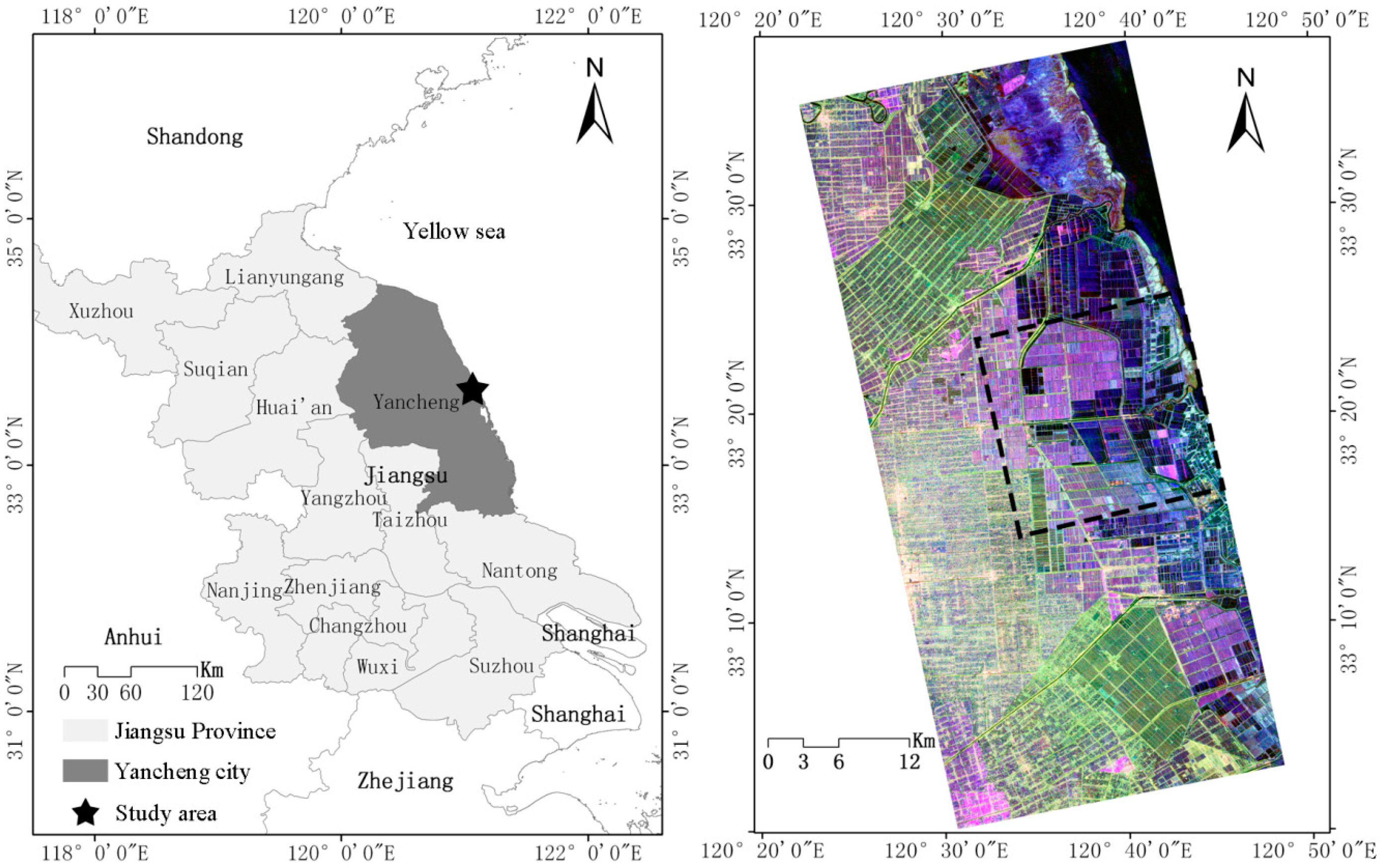
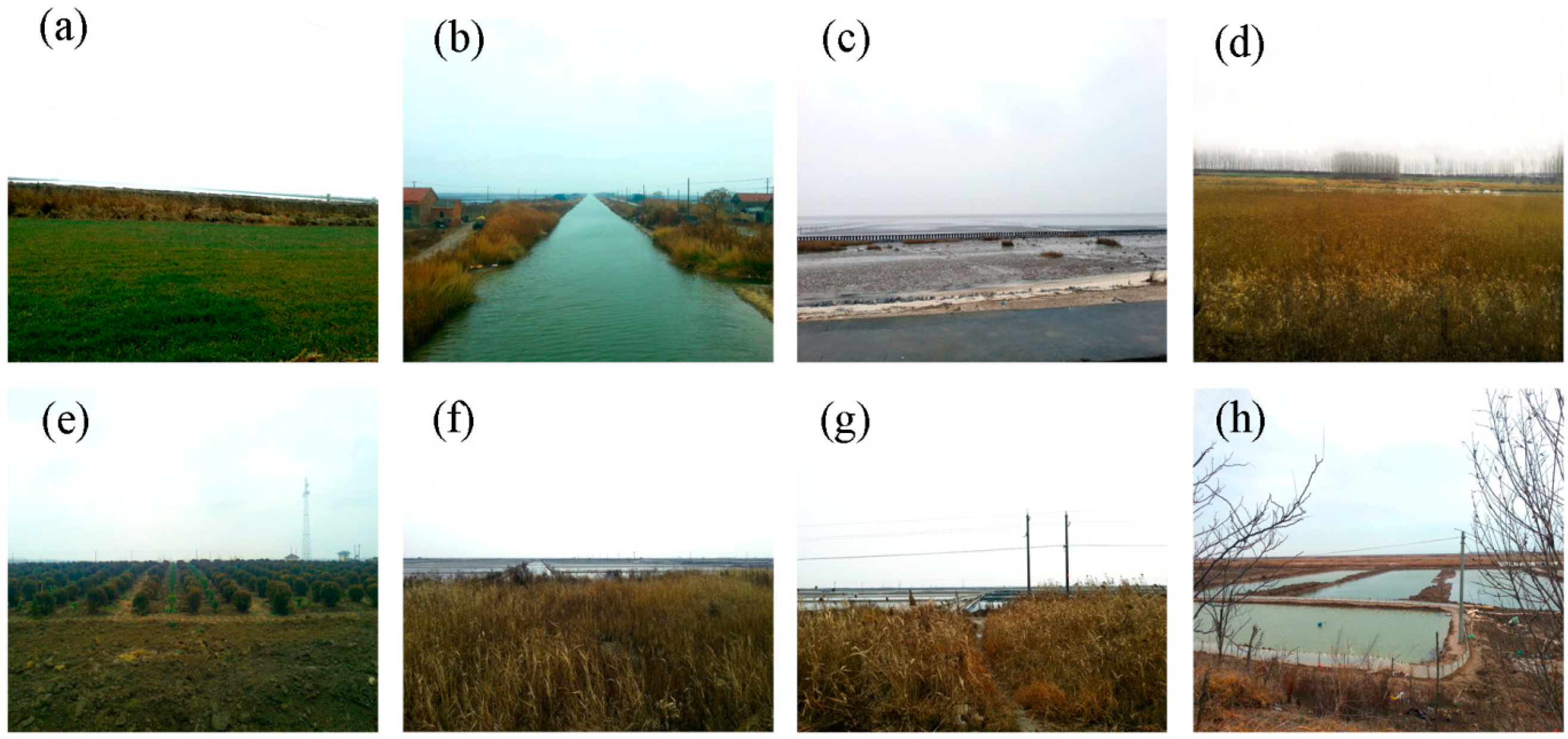
2. Study Area and Datasets

The experiment was conducted in the Yancheng National Nature Reserve, which is located along the eastern coast of China in the Yangtze River Basin. The study site covers approximately 17 km × 17 km and is approximately 270 km northwest of the city of Shanghai (Figure 1). The study area is within the transitional zone between terrestrial and aquatic ecosystems. The land use/land cover (LULC) types in the area can be divided into three groups: natural wetlands (wetland vegetation, rivers, sea and sand), artificial wetlands (paddy rice, irrigable land, fish ponds and grasslands) and non-wetland types (dry land and roads). Note that in this area, most of the grasslands are located on a farm and were classified as “artificial grasslands” (planted grass for grazing) in the second land survey in China. Therefore, the class was grouped into artificial wetlands here. The land cover in this area is diverse; some land cover types exhibit similar scattering mechanisms, which make them difficult to identify.

L-band fully polarimetric ALOS PALSAR data acquired in April, 2009, were used in this study. The incidence angle of the image was 23.858°, and the resolution was 9.37 m and 3.57 m in the range and azimuth directions, respectively. The original data were in single-look complex (SLC) format; thus, multi-look processing was completed with 6 looks in the azimuth direction and 1 look in the range direction to improve the image readability. To reduce noise, the refined Lee filter was employed in a 3 × 3 window [20,21]. ALOS multispectral image obtained in May 2008, and a satellite image from Google Earth were chosen as supplementary data to interpret the data visually and to facilitate the collection of ground-truth data during the field investigation.

Fieldwork was conducted on a date close to the image acquisition (March 2009) to collect ground-truth data. A total of 4610 samples of 10 land cover types were selected across the entire study area, and photographs of typical land cover were taken during the field investigation to assist in the image interpretation and analysis (Figure 2). Global positioning system (GPS) equipment was employed to record the coordinates of the collected samples. Hundreds of field plots for each class were collected. All of the field plots were randomly divided into two groups: one group included 2567 samples for building the decision tree, while the other group included 2043 samples for validating the classification results.

Figure 1. Map of the study area (left) and Pauli RGB image (right). The region of interest is shown in the black dashed rectangle.

Figure 1. Map of the study area (left) and Pauli RGB image (right). The region of interest is shown in the black dashed rectangle.

Figure 2. Photographs of eight typical land cover types taken in the study area. (a) Grassland; (b) river; (c) sand; (d) paddy rice; (e) irrigable land; (f) wetland vegetation; (g) dry land; and (h) fish pond.

Figure 2. Photographs of eight typical land cover types taken in the study area. (a) Grassland; (b) river; (c) sand; (d) paddy rice; (e) irrigable land; (f) wetland vegetation; (g) dry land; and (h) fish pond.

3. Methodology

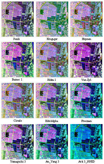
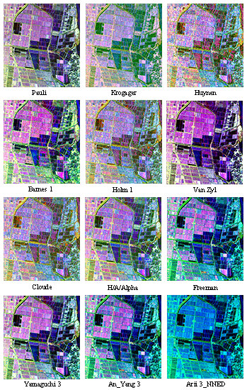
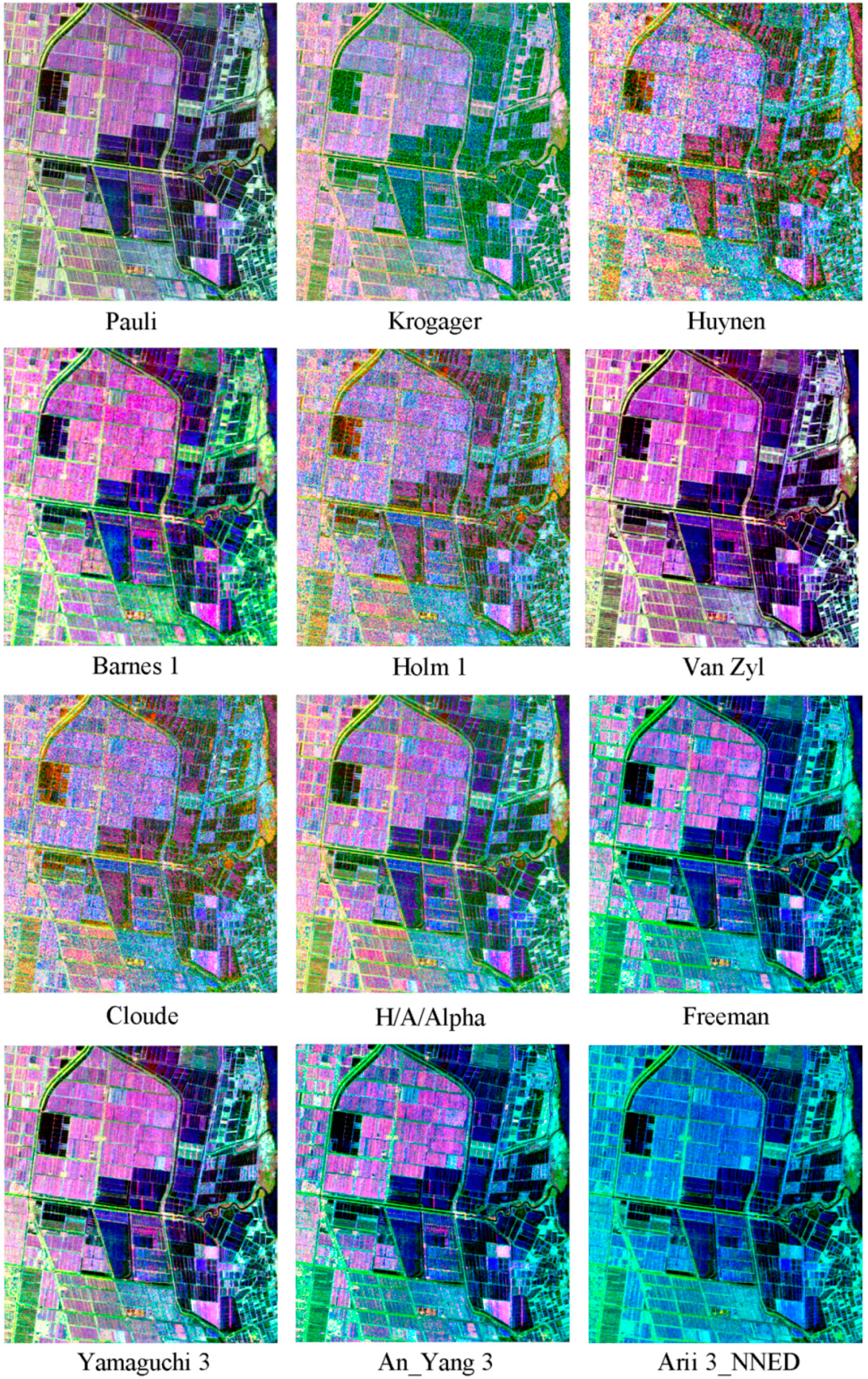
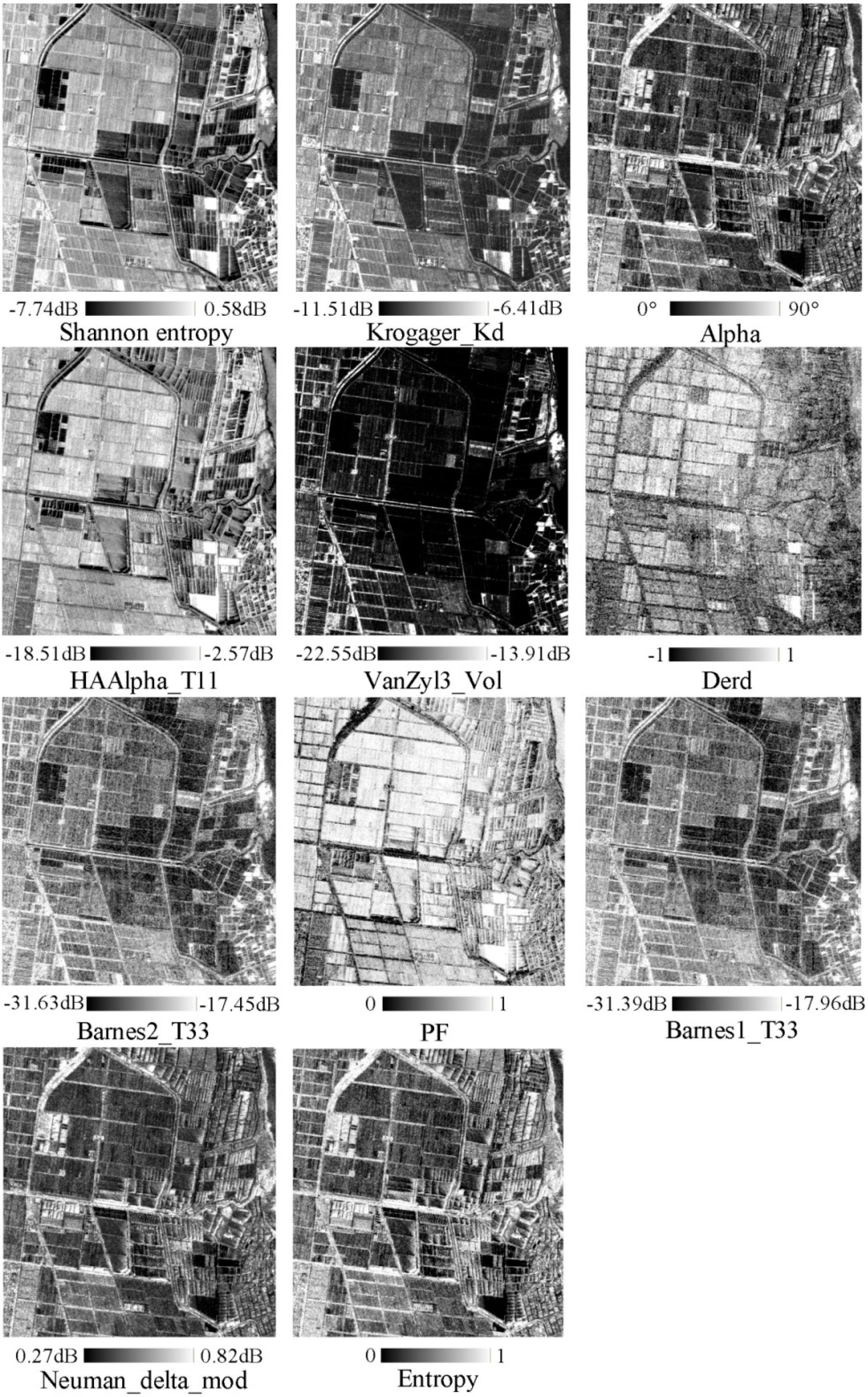
3.1. Polarimetric Decomposition and Parameter Extraction

Polarimetric decomposition is an important and continually developing information-extracting approach in PolSAR data analysis [22,23]. As one of the most popular decomposition methods, Pauli decomposition expresses the measured scattering matrix S in the so-called Pauli basis:

$${\text{σ}}_1=\left[\begin{array}{cc}1& 0\\ 0& 1\end{array}\right],{\text{ σ}}_2=\left[\begin{array}{cc}1& 0\\ 0& -1\end{array}\right],{\text{ σ}}_3=\left[\begin{array}{cc}0& 1\\ 1& 0\end{array}\right],{\text{ σ}}_4=\left[\begin{array}{cc}0& \text{i}\\ -\text{i}& 0\end{array}\right]$$

(1)

The 2 × 2 observed scattering matrix S can be vectorized to $\text{κ}$ with the Pauli basis.

$$\text{S}=\left[\begin{array}{cc}{S}_{hh}& S_{hv}\\ S_{vh}& S_{vv}\end{array}\right]$$

$$\text{κ}=V\left(\text{S}\right)=\frac{1}{\sqrt{2}}{\left[S_{hh}+S_{vv}, S_{hh}-S_{vv}, S_{hv}+S_{vh}, i(S_{hv}-S_{vh})\right]}^T$$

(2)

With the reciprocity theorem and $S_{hv}=S_{vh}$, the last element of vector $\text{κ}$ is zero. The remaining three elements, $S_{hh}+S_{vv}, S_{hh}-S_{vv}$ and $2S_{hv},$ are associated with three physical scattering mechanisms, which are odd-bounce scattering, double-bounce scattering and volume scattering, respectively. Thus, the Pauli RGB image (${\left|S_{hh}+S_{vv}\right|}^2\left(\text{Blue}\right), {\left|S_{hh}-S_{vv}\right|}^2\left(\text{Red}\right)$ and $2{\left|S_{hv}\right|}^2(\text{Green})$) can be utilized to interpret the physical information from a qualitative point of view.

In addition to the Pauli decomposition, many other polarimetric decompositions exist. The RGB composition images that correspond with several decompositions are displayed in Figure 3. However, as discussed in the references for Table 1, each decomposition has unique limitations. In addition, different polarimetric decompositions are sensitive to different land cover types [20]. Therefore, the method might be more effective in a study area with complex and diverse land cover types, such as wetland ecosystems, to integrate several different decompositions. In this study, 92 polarimetric parameters derived from 20 decompositions were explored for the LULC classification (Table 1 [22,24,25,26,27,28,29,30,31,32,33,34,35,36,37,38,39]). The parameters were merged with 6 coherency matrix elements to form a multi-layer image on which subsequent processing steps, including object-based analysis and feature extraction, operated.

Figure 3. RGB composition images of different polarimetric decompositions.

Figure 3. RGB composition images of different polarimetric decompositions.

Table 1. Polarimetric parameters extracted from 20 polarimetric decompositions.

Decomposition Method	Polarimetric Parameters
Pauli [22]	Pauli_a	Pauli_b	Pauli_c
Krogager [24]	Krogager_KS	Krogager_KD	Krogager_KH
Huynen [25]	Huynen_T11	Huynen_T22	Huynen_T33
Barnes1 [26]	Barnes1_T11	Barnes1_T22	Barnes1_T33
Barnes2 [26]	Barnes2_T11	Barnes2_T22	Barnes2_T33
Holm1 [27]	Holm1_T11	Holm1_T22	Holm1_T33
Holm2 [27]	Holm2_T11	Holm2_T22	Holm2_T33
VanZyl3 [28]	VanZyl3_Vol	VanZyl3_Odd	VanZyl3_Dbl
Cloude [22]	Cloude_T11	Cloude_T22	Cloude_T33
H/A/Alpha [29]	H/A/A_T11	H/A/A_T22	H/A/A_T33
	Entropy	Anisotropy	Shannon Entropy
	DERD	Polarization Asymmetry	Polarization Fraction
	SERD	Radar Vegetation Index	Anisotropy12
	Pedestal Height	Alpha ($\overline{\alpha }$, $\text{ α}$1, $\text{ α}$2, $\text{ α}$3)	Anisotropyluenebury
	Pseudo Probabilities (p1, p2, p3)
Freeman2 [30]	Freeman2_Vol	Freeman2_Ground
Freeman3 [31]	Freeman_Vol	Freeman_Odd	Freeman_Dbl
Yamaguchi3 [32]	Yamaguchi3_Vol	Yamaguchi3_Odd	Yamaguchi3_Dbl
Yamaguchi4 [33]	Yamaguchi4_Vol	Yamaguchi4_Odd	Yamaguchi4_Dbl
	Yamaguchi4_Hlx
Neumann [34]	Neumann_delta_mod	Neumann_delta_pha	Neumann_tau
Touzi [35]	TSVM_alpha_s	TSVM_alpha_s1	TSVM_alpha_s2
	TSVM_alpha_s3	TSVM_tau_m	TSVM_tau_m1
	TSVM_tau_m2	TSVM_tau_m3	TSVM_phi_s1
	TSVM_phi_s2	TSVM_phi_s3	TSVM_phi_s
	TSVM_psi1	TSVM_psi2	TSVM_psi3
	TSVM_psi
An_Yang3 [36]	An_Yang3_Vol	An_Yang3_Odd	An_Yang3_Dbl
An_Yang4 [37]	An_Yang4_Vol	An_Yang4_Odd	An_Yang4_Dbl
	An_Yang4_Hlx
Arii3_NNED [38]	Arii3_NNED_Vol	Arii3_NNED_Odd	Arii3_NNED_Dbl
Arii3_ANNED [39]	Arii3_ANNED_Vol	Arii3_ANNED_Odd	Arii3_ANNED_Odd

Table 1. Polarimetric parameters extracted from 20 polarimetric decompositions.

Decomposition Method	Polarimetric Parameters
Pauli [22]	Pauli_a	Pauli_b	Pauli_c
Krogager [24]	Krogager_KS	Krogager_KD	Krogager_KH
Huynen [25]	Huynen_T11	Huynen_T22	Huynen_T33
Barnes1 [26]	Barnes1_T11	Barnes1_T22	Barnes1_T33
Barnes2 [26]	Barnes2_T11	Barnes2_T22	Barnes2_T33
Holm1 [27]	Holm1_T11	Holm1_T22	Holm1_T33
Holm2 [27]	Holm2_T11	Holm2_T22	Holm2_T33
VanZyl3 [28]	VanZyl3_Vol	VanZyl3_Odd	VanZyl3_Dbl
Cloude [22]	Cloude_T11	Cloude_T22	Cloude_T33
H/A/Alpha [29]	H/A/A_T11	H/A/A_T22	H/A/A_T33
	Entropy	Anisotropy	Shannon Entropy
	DERD	Polarization Asymmetry	Polarization Fraction
	SERD	Radar Vegetation Index	Anisotropy12
	Pedestal Height	Alpha ($\overline{\alpha }$, $\text{ α}$1, $\text{ α}$2, $\text{ α}$3)	Anisotropyluenebury
	Pseudo Probabilities (p1, p2, p3)
Freeman2 [30]	Freeman2_Vol	Freeman2_Ground
Freeman3 [31]	Freeman_Vol	Freeman_Odd	Freeman_Dbl
Yamaguchi3 [32]	Yamaguchi3_Vol	Yamaguchi3_Odd	Yamaguchi3_Dbl
Yamaguchi4 [33]	Yamaguchi4_Vol	Yamaguchi4_Odd	Yamaguchi4_Dbl
	Yamaguchi4_Hlx
Neumann [34]	Neumann_delta_mod	Neumann_delta_pha	Neumann_tau
Touzi [35]	TSVM_alpha_s	TSVM_alpha_s1	TSVM_alpha_s2
	TSVM_alpha_s3	TSVM_tau_m	TSVM_tau_m1
	TSVM_tau_m2	TSVM_tau_m3	TSVM_phi_s1
	TSVM_phi_s2	TSVM_phi_s3	TSVM_phi_s
	TSVM_psi1	TSVM_psi2	TSVM_psi3
	TSVM_psi
An_Yang3 [36]	An_Yang3_Vol	An_Yang3_Odd	An_Yang3_Dbl
An_Yang4 [37]	An_Yang4_Vol	An_Yang4_Odd	An_Yang4_Dbl
	An_Yang4_Hlx
Arii3_NNED [38]	Arii3_NNED_Vol	Arii3_NNED_Odd	Arii3_NNED_Dbl
Arii3_ANNED [39]	Arii3_ANNED_Vol	Arii3_ANNED_Odd	Arii3_ANNED_Odd

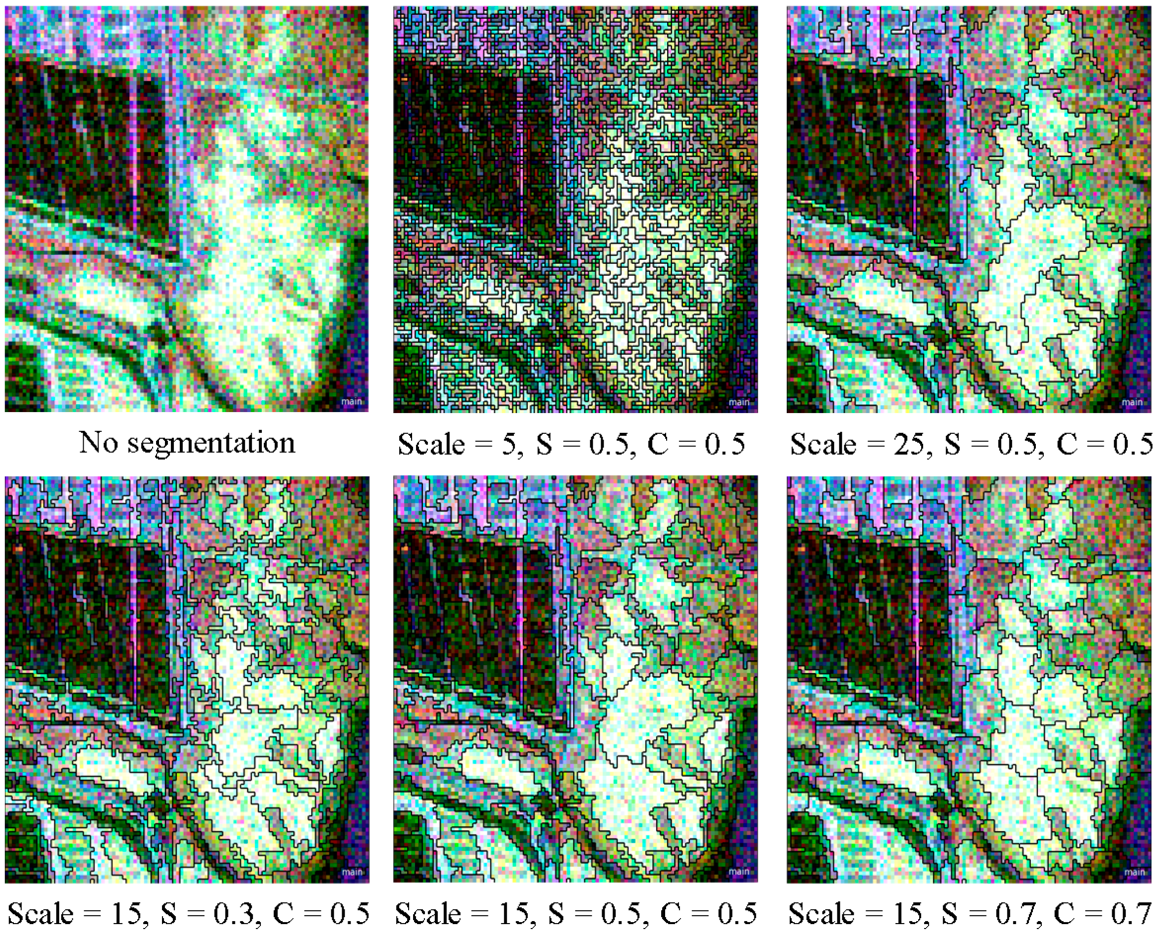
3.2. Object-Based Image Analysis and Feature Calculation

Object-based analysis of meaningful image objects with adjacent pixels and homogeneous values, rather than single pixels, can improve the accuracy of LULC classification [13,15,40]. A perfect meaningful image object represents exactly one specific category. The image object is expected to be as large as possible and to exhibit the typical shape of the land cover type. Thus, the performance of object-based classification depends on the quality of the image segmentation [18]. In this study, the multi-resolution segmentation module provided in eCognition [41] was employed to perform the object-based segmentation and analysis.

Too many layers in the segmentation can greatly increase the computations and distort the segmentation performance. As noted, a Pauli RGB image can represent all polarimetric information embedded in polarization measurements and retain subtle details in the features; thus, this image is always employed when qualitatively interpreting the physical meanings of the land cover. Therefore, we opted to employ the Pauli RGB image for segmentation. Each channel of the Pauli RGB image was equally weighted during the segmentation, as they were equally sensitive to the three scattering mechanisms.

Scale parameters of 5, 15 and 25 were set to test the segmentation (Figure 4). With a scale of 5, the land parcels were too fragmented to reflect the shape of the land cover, and with a scale of 25, the image objects were so large, that many details were lost. The optimal segmentation scale in this experiment was 15 according to a visual inspection. Furthermore, according to our tests, a weight of 0.5 was given to the shape and compactness criterion to optimally fit the objects.

Figure 4. Determining the optimal scale for the Pauli RGB image segmentation.

Figure 4. Determining the optimal scale for the Pauli RGB image segmentation.

Statistical (layer values), geometric, textural and class-related features of image objects were extracted to build the decision tree. Four indicators were related to the statistical values of each object: the minimum, maximum, mean and standard deviation of each layer. We used 57 geometric features, including area, length/width, shape index, border length and density. Eight textural features were extracted by a grey-level co-occurrence matrix (GLCM) algorithm, including entropy, dissimilarity, contrast, homogeneity, second moment, mean, standard deviation and correlation. Seven class-related indicators were obtained, such as the existence of neighbor objects, the number of neighbor objects and the distance to neighbor objects. The total number of features extracted from the combined multi-layer image was 1919. Commonly-used features are the mean value $\overline{C_L}$ and the standard deviation ${\text{σ}}_L$, which can be calculated by the layer value $C_{Li}$ of n pixels contained in an object.

$$\overline{C_L}=\frac{1}{n}\times {\displaystyle \sum }_{i=1}^n{C}_{Li}$$

(3)

$${\text{σ}}_L=\sqrt{\frac{1}{n}\times ({\displaystyle \sum }_{i=1}^n{C_{Li}}^2-\frac{1}{n}{\displaystyle \sum }_{i=1}^n{C}_{Li}{\displaystyle \sum }_{i=1}^n{C}_{Li})}$$

(4)

The shape index, which is used to describe the compactness of an object’s boundary, is particularly useful for distinguishing land cover with different shapes. The shape index is defined as:

$$\text{S}=\frac{e}{4\sqrt{A}}$$

(5)

where $e$ and A are the perimeter and the area of an object, respectively.

3.3. Decision Tree Algorithm

The decision tree model, also known as a rule-based model, builds a classification tree by learning via training samples; the model completes the classification based on the developed rules [42]. Decision tree learning has been one of the most successful techniques for supervised classification. The technique is used to find the optimal solution of a Bayesian decision problem, i.e., to select an optimal solution from several decision alternatives. In this research, 1919 features were extracted from the PolSAR data; thus, how to select the optimal features for the LULC classification was a challenge. Here, QUEST [43], which is a binary-split and relatively automatic “machine learning” decision tree method, was employed for optimal feature selection and decision tree building. QUEST can be employed with univariate or linear combination splits, and the attribute selection method has negligible bias. Each attribute has an approximately equal chance of being selected to split a node if all attributes are uninformative with respect to the class. Compared with other tree-building techniques, QUEST can easily handle categorical predictor variables with many categories, and the built trees are relatively simple to interpret by non-statisticians.

3.4. Methods for Comparison

To demonstrate the efficiency of the proposed method and the contributions of polarimetric parameters and object-based analysis to the classification performance, a series of comparisons were conducted with five other methods: the Wishart supervised classification (WSC), the proposed method without polarimetric parameters (PWPP), the proposed method without an object-based segmentation (PWOS), the proposed method without textural and geometric information (PWTG) and the proposed method using the nearest-neighbor classifier instead of the decision tree algorithm (PNNC). The Wishart supervised method is a frequently-used PolSAR classification. It is a Bayes maximum likelihood classifier that is based on the complex Wishart distribution for the polarimetric coherency matrix [44]. The PWPP method was applied based on the coherency matrix elements using the processes of object-based analysis and the decision tree algorithm. In the PWOS method, polarimetric decomposition and the decision tree algorithm were applied to the PolSAR data without an object-based analysis. The PWTG method invoked similar processes to the proposed method; however, textural and geometric features were not incorporated. The nearest-neighbor classifier is commonly used in object-based analysis. In this study, the PNNC method was employed for a comparison by using the nearest-neighbor classifier instead of the decision tree algorithm. The feature space optimization function provided in eCognition was utilized for the optimal feature selection in the nearest-neighbor classifier.

4. Results and Discussion

4.1. Constructed Decision Tree and Selected Polarimetric Parameters

In this study, 2567 training samples for 10 land cover types (wetland vegetation, rivers, sea, sand, paddy rice, dry land, irrigable land, fish ponds, grasslands and roads) were used to build the decision tree (see Supplemental Table S1). During the tree development, the depth was set to five to avoid over-fitting. To generate a simple tree, the method of “cost-complexity” pruning was employed based on 10-fold cross-validation. The structure of the final decision tree is shown in Figure 5. As presented in the figure, the layer mean values for the Shannon entropy, Krogager_Kd, Barnes2_T33, Alpha, HAAlpha_T11, polarization fraction, VanZyl3_Vol, Derd, Barnes1_T33, Neuman_delta_mod, the standard deviation of entropy, the shape index and the distance to neighbor objects were selected for the decision tree. The optimal polarimetric parameters selected by the QUEST algorithm are displayed in Figure 6.

Figure 5. Structure of the decision tree. SE, Shannon entropy; KG, Krogager_Kd; B2, Barnes2_T33; HAA, HAAlpha_T11; PF, Polarization Fraction; VZ, VanZyl3_Vol; B1, Barnes1_T33; NDM, Neuman_delta_mod; SD, the standard deviation of entropy; DS, the distance to the neighbor objects.

Figure 5. Structure of the decision tree. SE, Shannon entropy; KG, Krogager_Kd; B2, Barnes2_T33; HAA, HAAlpha_T11; PF, Polarization Fraction; VZ, VanZyl3_Vol; B1, Barnes1_T33; NDM, Neuman_delta_mod; SD, the standard deviation of entropy; DS, the distance to the neighbor objects.

The radar signals returned from the vegetation-covered area, such as paddy rice, irrigable land, dry land and wetland vegetation, include the vegetation canopy backscatter (volume scattering) and trunk-water or trunk-ground backscatter (double-bounce scattering). The backscatter from grasslands and sand is mainly single-bounce scattering, which is greatly influenced by the soil surface. Water bodies, such as fish ponds, rivers and the sea, generally exhibit low return scattering; these areas are mostly dark on the PolSAR image. The scattering on roads is mainly double-bounced due to the interaction with telegraph poles and trees on either side, so they are shown as bright lines on radar imagery. Overall, the land cover types in this study area are complex, and some of them exhibit similar physical scattering mechanisms; thus, it is difficult to distinguish land cover classes accurately by using polarimetric scattering information alone.

Figure 6. Polarimetric parameters selected in the decision tree.

Figure 6. Polarimetric parameters selected in the decision tree.

Shannon entropy is a measurement that was introduced by Morio et al. [45]; it is the sum of two contributions related to intensity and polarimetry. The intensity contribution depends on the total backscattering power, and the polarimetric contribution depends on the Barakat degree of polarization. The training samples could be classified into two groups by the mean value of the Shannon entropy with a threshold of −3.01. Crop fields that are near water bodies could not be differentiated from water. Corresponding to the contribution of the di-plane component in the Krogager decomposition [24], the mean value of Krogager_Kd was helpful in distinguishing water bodies and vegetation. In the right branch of the mean value of Krogager_Kd, vegetation could be identified, as it had stronger double-bounce scattering (trunk-water or trunk-ground backscatter) than the water bodies in the left branch. Representing the averaged scattering mechanisms from surface scattering to double-bounce scattering, the mean value of Alpha with the threshold of 31.511 was used to divide the water bodies into two groups. The left branch included grasslands and water, the dominant scattering of which should be single bounce. However, the trails across fish ponds presented a slight volume scattering. Thus, the mean value of VanZyl_Vol could be used to distinguish water bodies from nearby grasslands. The entropy (H) represents the randomness of a scattering medium, from isotropic scattering (H = 0) to totally random scattering (H = 1) [44]. For smoother surfaces, such as the ocean, surface scattering dominates and H is near zero. As mentioned, fish ponds presented a slight volume scattering in this study area, so compared with the sea, fish ponds had higher entropy values. The standard deviation of entropy is calculated from the entropy and is more sensitive to the variation in surface roughness. Thus, the standard deviation of entropy was helpful in further classifying the sea and fish ponds. With a relatively compact shape, a fish pond could be easily distinguished from a river by using the shape index. The mean value of Alpha and the distance to the sea could successfully differentiate herbaceous wetland vegetation from artificial grasslands. According to knowledge, wetland vegetation grows on the coast near the sea, and the artificial grasslands are located on farms far from the sea, so the distance to the sea can be regarded as an important spatial indicator to reduce the confusion between artificial grasslands and wetland vegetation. When the distance between an object and the sea was less than 70 pixels, the object was regarded as wetland vegetation; otherwise, the object was grassland. The double-bounce eigenvalue relative difference (Derd), which was introduced by Allain et al. [46], is very sensitive to surface roughness. In the study, the mean value of Derd was used twice to classify paddy rice, irrigable land and dry land, all of which had similar dominant scattering mechanisms, but different surface roughness.

The classes in the right branch of the Shannon entropy node, such as roads, sand and paddy rice, could be divided into two groups according to the mean value of Barnes2_T33. The parameter, polarization fraction (PF), ranged between zero and one [47]. When the third eigenvalue (${\text{λ}}_3$) of the coherency matrix was zero, the entire radar return was polarized. When ${\text{λ}}_3$ was greater than zero, the value of PF dropped. As shown in Figure 6 (PF), roads exhibited lower PF than paddy rice and dry land. As a result, the mean value of PF could be used to reduce the confusion between farmland and roads. With similar scattering mechanisms, but different surface roughness and soil moisture, paddy rice and dry land could be distinguished by employing the mean value of Derd. Figure 6 shows that the sand and paddy rice were relatively homogeneous in the HAAlpha_T11 image, so the mean value of HAAlpha_T11 could be used to separate roads from paddy rice and sand. Corresponding to pure targets, Barnes1_T33 was useful in further distinguishing sand from paddy rice. The Neumann decomposition, which is a simple vegetation model for polarimetric covariance or coherency matrix elements, was originally intended for volumetric distributed targets in terms of second-order statistics. As a general scattering mechanism indicator, Neumann_delta_mod was helpful in identifying some paddy fields, which typically had stronger volume scattering than roads.

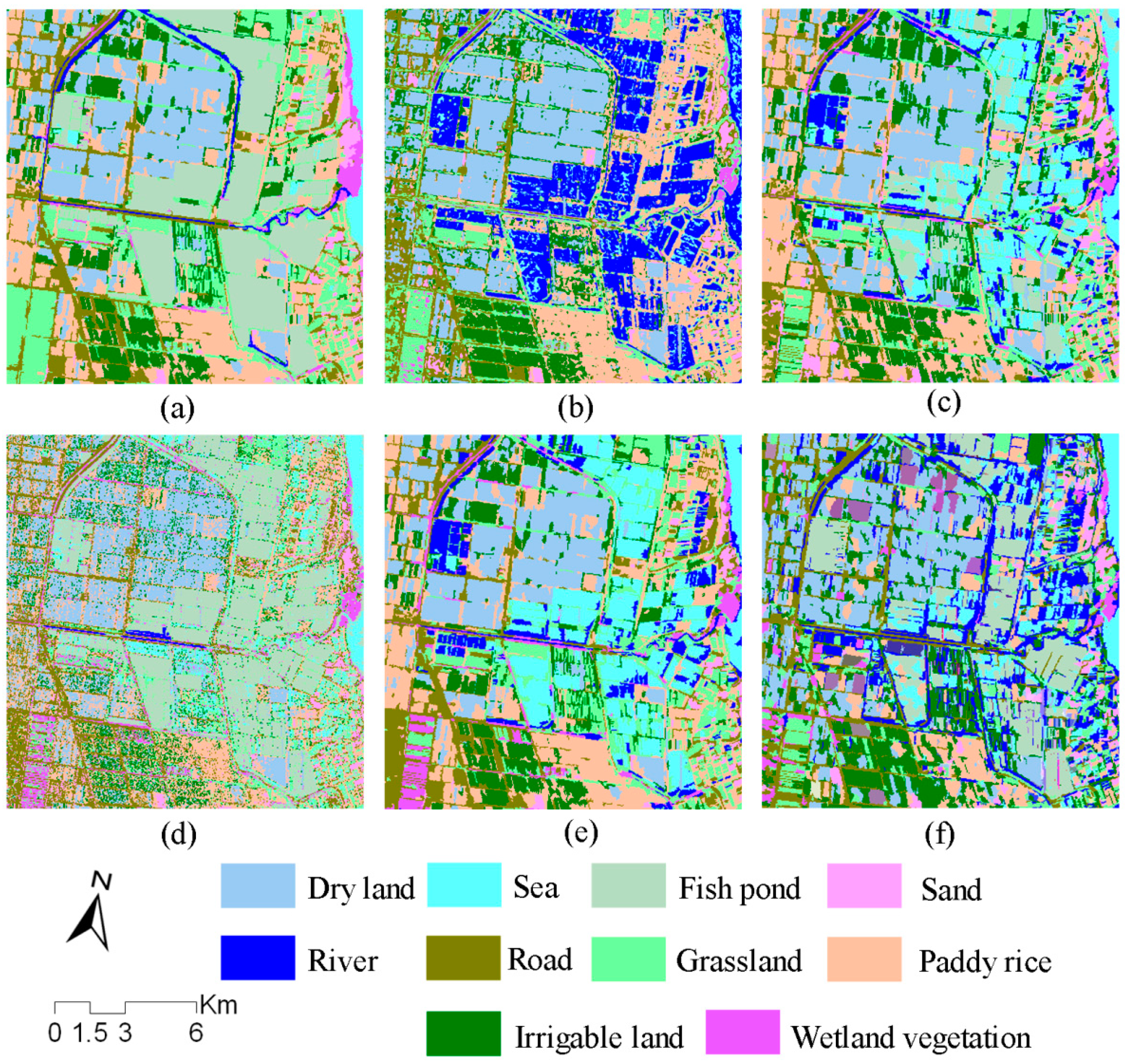
4.2. LULC Classification Results

The LULC classification results from the proposed method and five other methods are displayed in Figure 7 and Table 2 (and see Supplemental Tables S2–S7 for detailed results from individual methods). A total of 2043 field samples were collected to calculate the classification accuracy (Tables S1), including overall accuracy (OA), producer’s accuracy (PA) and user’s accuracy (UA). The analysis and discussion are based on visual interpretations and quantitative comparisons. As seen from the comparison between the proposed method and WSC method, the overall accuracy for the latter method was 66.6%, which was lower than that of the proposed method (87.3%). In addition, the producer’s and user’s accuracies for most classes decreased with the WSC method. In particular, fish ponds, the sea and rivers were grouped into one class due to their similar backscatter values (Figure 7b). Given that soil moisture is a crucial factor that generally affects the land cover scattering type, grasslands have lower soil moisture than paddy rice. In Figure 7b, however, some artificial grasslands could not be differentiated from paddy rice by only using scattering mechanisms, perhaps because the PolSAR data were acquired in April when little water was present in the paddy fields. Furthermore, some bare lands that exhibited dominant single-bounce scattering were observed in the paddy rice during the fieldwork. As a result, some of the paddy rice showed similar scattering to artificial grasslands. This comparison demonstrated the effects of integrating the polarimetric decomposition, object-based analysis and decision tree algorithm.

Figure 7. Classification results from: (a) the proposed method; (b) the Wishart supervised classification; (c) the proposed method without polarimetric parameters; (d) the proposed method without an object-based segmentation; (e) the proposed method without textural and geometric information; and (f) the proposed method using the nearest neighbor classifier instead of the decision tree algorithm.

Figure 7. Classification results from: (a) the proposed method; (b) the Wishart supervised classification; (c) the proposed method without polarimetric parameters; (d) the proposed method without an object-based segmentation; (e) the proposed method without textural and geometric information; and (f) the proposed method using the nearest neighbor classifier instead of the decision tree algorithm.

The results of the proposed method and PWPP method were compared to verify the improvement after polarimetric parameters were included in the LULC classification. From Table 2, the producer’s and user’s accuracies for almost all land cover types decreased when the polarimetric parameters were not used in the classification. Moreover, the overall accuracy decreased by 13.3% compared with the proposed method. Specifically, as observed in Figure 7c and Table 2, fish ponds achieved rather low accuracies due to their confusion with the sea. The user’s accuracy of fish ponds with the PWPP method was 24.6%, and the producer’s accuracy of the sea was 49.2%; in the proposed method, these accuracies increased to 89.5% and 88.8%, respectively. Entropy, which is a polarimetric parameter derived from the Cloude–Pottier decomposition, was useful in identifying fish ponds and the sea (Figure 5). The mean value of Derd helped distinguish paddy rice and dry land. In the proposed method, the producer’s and user’s accuracies of dry land were 88.8% and 87.1%, respectively, while in the PWPP method, the two indicators decreased to 79.4% and 84.3%, respectively. For paddy rice, the two indicators were 84.9% and 90.9%, respectively, in the proposed method, but decreased to 75.7% and 71.6%, respectively, with the PWPP method. The improvement in the accuracies for roads and paddy rice indicated that the mean value of Neumann_delta_mod was useful in separating these classes. Overall, the polarimetric parameters selected by the QUEST algorithm were highly important in reducing land cover confusion and improving the classification performance in the coastal wetlands.

Table 2. Classification accuracy. SA, sand; DL, dry land; FP, fish pond; GL, grassland; IL, irrigable land; PR, paddy rice; RI, river; RO, road; S, sea; W, wetland vegetation; WSC, Wishart supervised classification; PWPP, proposed method without polarimetric parameters; PWOS, proposed method without object-based segmentation; PWTG, proposed method without textural and geometric information; PNNC, proposed method with the nearest-neighbor classifier.

Method	Accuracy	Class
		SA	DL	FP	GL	IL	PR	RI	RO	S	W
Proposed method	PA (%)	83.2	88.8	86.0	84.6	80.3	84.9	95.3	92.0	88.8	93.5
	UA (%)	89.2	87.1	89.5	86.4	87.4	90.9	85.5	85.2	90.0	80.7
	OA (%)	87.3
WSC	PA (%)	84.3	77.9	42.8	75.4	76.1	74.1	30.3	89.3	52.3	94.6
	UA (%)	83.4	87.2	6.6	78.8	87.4	71.6	80.7	87.9	17.3	72.5
	OA (%)	66.6
PWPP	PA (%)	88.6	79.4	73.6	74.4	67.9	75.7	73.4	91.1	49.2	89.3
	UA (%)	83.0	84.3	24.6	67.6	90.6	71.6	80.7	92.1	79.6	72.5
	OA (%)	74.0
PWOS	PA (%)	90.6	78.8	92.6	72.8	69.4	82.4	51.6	90.7	55.6	92.1
	UA (%)	79.6	84.8	82.5	67.6	90.6	78.8	23.4	93.2	89.0	77.6
	OA (%)	77.1
PWTG	PA (%)	87.8	79.9	61.6	71.8	71.2	75.7	75.6	90.1	47.6	84.5
	UA (%)	84.4	87.1	14.0	65.6	87.4	71.7	80.8	92.1	84.1	72.5
	OA (%)	73.2
PNNC	PA (%)	87.6	80.5	94.6	70.7	65.5	89.5	65.7	90.3	82.6	94.4
	UA (%)	79.5	83.8	69.7	67.1	91.7	81.2	81.8	88.4	84.6	77.8
	OA (%)	80.5

Table 2. Classification accuracy. SA, sand; DL, dry land; FP, fish pond; GL, grassland; IL, irrigable land; PR, paddy rice; RI, river; RO, road; S, sea; W, wetland vegetation; WSC, Wishart supervised classification; PWPP, proposed method without polarimetric parameters; PWOS, proposed method without object-based segmentation; PWTG, proposed method without textural and geometric information; PNNC, proposed method with the nearest-neighbor classifier.

Method	Accuracy	Class
		SA	DL	FP	GL	IL	PR	RI	RO	S	W
Proposed method	PA (%)	83.2	88.8	86.0	84.6	80.3	84.9	95.3	92.0	88.8	93.5
	UA (%)	89.2	87.1	89.5	86.4	87.4	90.9	85.5	85.2	90.0	80.7
	OA (%)	87.3
WSC	PA (%)	84.3	77.9	42.8	75.4	76.1	74.1	30.3	89.3	52.3	94.6
	UA (%)	83.4	87.2	6.6	78.8	87.4	71.6	80.7	87.9	17.3	72.5
	OA (%)	66.6
PWPP	PA (%)	88.6	79.4	73.6	74.4	67.9	75.7	73.4	91.1	49.2	89.3
	UA (%)	83.0	84.3	24.6	67.6	90.6	71.6	80.7	92.1	79.6	72.5
	OA (%)	74.0
PWOS	PA (%)	90.6	78.8	92.6	72.8	69.4	82.4	51.6	90.7	55.6	92.1
	UA (%)	79.6	84.8	82.5	67.6	90.6	78.8	23.4	93.2	89.0	77.6
	OA (%)	77.1
PWTG	PA (%)	87.8	79.9	61.6	71.8	71.2	75.7	75.6	90.1	47.6	84.5
	UA (%)	84.4	87.1	14.0	65.6	87.4	71.7	80.8	92.1	84.1	72.5
	OA (%)	73.2
PNNC	PA (%)	87.6	80.5	94.6	70.7	65.5	89.5	65.7	90.3	82.6	94.4
	UA (%)	79.5	83.8	69.7	67.1	91.7	81.2	81.8	88.4	84.6	77.8
	OA (%)	80.5

The PWOS method was used for the LULC classification by applying similar operations to the proposed method, including polarimetric decomposition and the decision tree algorithm; however, the object-based segmentation was not employed. Regarding the comparison between the object-based (the proposed method) and pixel-based (the PWOS method) classifications, Figure 7d and the accuracy evaluation in Table 2 show that the performance of the proposed method was generally enhanced. The overall accuracy of the PWOS method had an accuracy of 77.1%, which was 10.2% lower than the proposed method. Specifically, the PWOS method failed to correctly distinguish rivers, roads and grasslands due to the limitation of using only single-pixel information. More importantly, there was a mass of isolated points in Figure 7d compared with Figure 7a, which provided powerful evidence that the object-based method was less affected by noise in the SAR image. Figure 7a had lower spatial heterogeneity compared with Figure 7d, and the proposed method represented reality more accurately than the pixel-based method. These results proved the importance of the object-based method in PolSAR LULC classification.

When textural and geometric information were not employed in the classification, the overall accuracy of the PWTG method was 73.2%, which was 14.1% lower than the proposed method. As displayed in Figure 7e, some rivers could not be separated from fish ponds by merely using polarimetric information, because both were dominated by single-bounce scattering. Because the shapes of these two land cover types are significantly different, the shape index could be used to distinguish them. The producer’s and user’s accuracies of fish ponds were 61.6% and 14.0% with PWTG, respectively; after the shape index was added to the classification, the two indicators increased to 86.0% and 89.5%, respectively. Some wetland vegetation areas were confused with grasslands when using the PWTG method, because their scattering mechanisms were similar. Based on knowledge and reference maps, wetland vegetation grows on the beach near the sea and grasslands are located on farms far from the sea, so the distance to the sea can be regarded as an important criterion for discriminating herbaceous vegetation-covered wetlands and grasslands (Figure 5). The accuracies of the two land cover types displayed in Table 2 also demonstrate this point. This comparison noted that the spatial relationships of the segmented objects could be used to improve the classification accuracies.

A comparison was also made between the proposed method and the PNNC method. In the latter method, the nearest-neighbor classifier replaced the decision tree algorithm, and the feature selection method was the feature space optimization function provided in eCognition. From Table 2, the overall accuracy of the PNNC method was 80.5%, which decreased by 6.8% compared with the proposed method. The classification results of irrigable land and roads using the PNNC method were slightly higher than those using the proposed method. However, for most of the land cover types, the proposed method obtained higher producer’s and user’s accuracies than the PNNC method.

5. Conclusions

An object-based classification scheme that integrates polarimetric decomposition and a decision tree algorithm was developed for land cover classification in coastal wetlands using fully polarimetric ALOS PALSAR data. The comparisons and analyses indicated that each component of the proposed method was highly important to the final classification results.

Compared with the Wishart supervised classification, the proposed method achieved higher producer’s and user’s accuracies for almost all of the land cover types. Moreover, the overall accuracy of the proposed method improved by 20.7%. The polarimetric parameters derived from the different decompositions were helpful in LULC classifications in coastal wetland areas. The parameter Derd was very useful in separating paddy rice from dry land. Entropy, which is decomposed from the Cloude–Pottier method, played a key role in distinguishing the sea and fish ponds. VanZyl_Vol and Alpha could be used to reduce the confusion between grasslands and other land cover types. Object-based analysis was robust, even with noise in the data, and produced more realistic results than pixel-based methods. The comparison between the proposed method and PWOS method strongly proved the advantages of object-based segmentation in classification of PolSAR data. Because the object-based analysis considered meaningful objects, it fully utilized statistical characteristics, textural features and geometric relationships. The comparison between the proposed method and PWTG method showed that the extracted geometric features greatly improved the classification performance. For instance, the shape index could differentiate rivers from fish ponds, both of which had the same return-scattering mechanism, but different shapes. The distance to the sea reduced the confusion between herbaceous vegetation-covered wetlands and grasslands. Although the PNNC method yielded satisfactory results with an overall accuracy of 80.5%, our analysis showed that the proposed method had the best performance. Moreover, the optimal features selection approach based on the QUEST algorithm was efficient, and the decision tree algorithm provided clear rules for implementing the LULC classification.

Overall, the findings in this study demonstrated that various polarimetric parameters and the object-based approach significantly contribute to coastal LULC classification when using fully polarimetric ALOS PALSAR data. Future studies should include testing the applicability of the proposed method in other study areas, employing other novel classification algorithms and mining the potential of alternative-frequency PolSAR images (C- and P-bands) in LULC classification.

References

1. Mitsch, W.J.; Gosselink, J.G. The value of wetlands: Importance of scale and landscape setting. Ecol. Econ. 2000, 35, 25–33. [Google Scholar] [CrossRef]
2. Awange, J.L.; Kiema, J.B.K. Marine and coastal resources. In Environmental Geoinformatics; Springer-Verlag: Berlin Heidelberg, Germany, 2013; pp. 397–413. [Google Scholar]
3. Ozesmi, S.; Bauer, M. Satellite remote sensing of wetlands. Wetl. Ecol. Manag. 2002, 10, 381–402. [Google Scholar] [CrossRef]
4. Wang, H.; Huang, J. Study on characteristics of land cover change using MODIS NDVI time series. J. Zhejiang Univ. Sci. A 2009, 35, 105–110. [Google Scholar]
5. Byrd, K.B.; O’Connell, J.L.; di Tommaso, S.; Kelly, M. Evaluation of sensor types and environmental controls on mapping biomass of coastal marsh emergent vegetation. Remote Sens. Environ. 2014, 149, 166–180. [Google Scholar] [CrossRef]
6. Dabrowska-Zielinska, K.; Budzynska, M.; Tomaszewska, M.; Bartold, M.; Gatkowska, M.; Malek, I.; Turlej, K.; Napiorkowska, M. Monitoring wetlands ecosystems using ALOS PALSAR (L-Band, HV) supplemented by optical data: A case study of Biebrza Wetlands in northeast Poland. Remote Sens. 2014, 6, 1605–1633. [Google Scholar] [CrossRef]
7. Zhang, H.; Zhang, Y.; Lin, H. A comparison study of impervious surfaces estimation using optical and SAR remote sensing images. Int. J. Appl. Earth Obs. Geoinf. 2012, 18, 148–156. [Google Scholar] [CrossRef]
8. Gosselin, G.; Touzi, R.; Cavayas, F. Polarimetric Radarsat-2 wetland classification using the Touzi decomposition: Case of the Lac Saint-Pierre Ramsar wetland. Can. J. Remote Sens. 2014, 39, 491–506. [Google Scholar] [CrossRef]
9. Touzi, R.; Deschamps, A.; Rother, G. Wetland characterization using polarimetric RADARSAT-2 capability. Can. J. Remote Sens. 2007, 33, S56–S67. [Google Scholar] [CrossRef]
10. Yajima, Y.; Yamaguchi, Y.; Sato, R.; Yamada, H.; Boerner, W.M. POLSAR image analysis of wetlands using a modified four-component scattering power decomposition. IEEE Trans. Geosci. Remote Sens. 2008, 46, 1667–1673. [Google Scholar] [CrossRef]
11. Cable, J.; Kovacs, J.; Shang, J.; Jiao, X. Multi-temporal polarimetric RADARSAT-2 for land cover monitoring in northeastern Ontario. Canada. Remote Sens. 2014, 6, 2372–2392. [Google Scholar] [CrossRef]
12. Van Beijma, S.; Comber, A.; Lamb, A. Random forest classification of salt marsh vegetation habitats using quad-polarimetric airborne SAR, elevation and optical RS data. Remote Sens. Environ. 2014, 149, 118–129. [Google Scholar] [CrossRef]
13. Benz, U.C.; Hofmann, P.; Willhauck, G.; Lingenfelder, I.; Heynen, M. Multi-resolution, object-oriented fuzzy analysis of remote sensing data for GIS-ready information. ISPRS J. Photogramm. Remote Sens. 2004, 58, 239–258. [Google Scholar] [CrossRef]
14. Peña, J.M.; Gutiérrez, P.A.; Hervás-Martínez, C.; Six, J.; Plant, R.E.; López-Granados, F. Object-based image classification of summer crops with machine learning methods. Remote Sens. 2014, 6, 5019–5041. [Google Scholar] [CrossRef]
15. Ban, Y.; Hu, H.; Rangel, I.M. Fusion of Quickbird MS and RADARSAT SAR data for urban land-cover mapping: Object-based and knowledge-based approach. Int. J. Remote Sens. 2010, 31, 1391–1410. [Google Scholar] [CrossRef]
16. Shi, W.; Yang, B.; Li, Q. An object-oriented data model for complex objects in three-dimensional geographical information systems. Int. J. Geogr. Inf. Sci. 2003, 17, 411–430. [Google Scholar] [CrossRef]
17. Benz, U.; Pottier, E. Object based analysis of polarimetric SAR data in alpha-entropy-anisotropy decomposition using fuzzy classification by eCognition. In Proceedings of the International Geoscience and Remote Sensing Symposium (IGARSS), Sydney, Australia, 9–13 July 2001; pp. 1427–1429.
18. Niu, X.; Ban, Y. Multi-temporal RADARSAT-2 polarimetric SAR data for urban land-cover classification using an object-based support vector machine and a rule-based approach. Int. J. Remote Sens. 2012, 34, 1–26. [Google Scholar] [CrossRef]
19. Qi, Z.; Yeh, A.G.O.; Li, X.; Lin, Z. A novel algorithm for land use and land cover classification using RADARSAT-2 polarimetric SAR data. Remote Sens. Environ. 2012, 118, 21–39. [Google Scholar] [CrossRef]
20. Lee, J.S.; Pottier, E. Polarimetric SAR speckle filtering. In Polarimetric Radar Imaging: From Basics to Applications, 1st ed.; CRC Press: London, UK, 2009; pp. 161–165. [Google Scholar]
21. Sartori, L.R.; Imai, N.N.; Mura, J.C.; Novo, E.M.L.M.; Silva, T.S.F. Mapping macrophyte species in the Amazon Floodplain wetlands using fully polarimetric ALOS/PALSAR data. IEEE Trans. Geosci. Remote Sens. 2011, 49, 4717–4728. [Google Scholar] [CrossRef]
22. Cloude, S.R.; Pottier, E. A review of target decomposition theorems in radar polarimetry. IEEE Trans. Geosci. Remote Sens. 1996, 34, 498–518. [Google Scholar] [CrossRef]
23. Cloude, S.R.; Pottier, E. An entropy based classification scheme for land applications of polarimetric SAR. IEEE Trans. Geosci. Remote Sens. 1997, 35, 68–78. [Google Scholar] [CrossRef]
24. Krogager, E. New decomposition of the radar target scattering matrix. Electron. Lett. 1990, 26, 1525–1527. [Google Scholar] [CrossRef]
25. Huynen, J.R. The Stokes matrix parameters and their interpretation in terms of physical target properties. In Proceedings of the Journées Internationales de la Polarimétrie Radar, Nantes, France, 20–22 March 1990.
26. Barnes, R.M. Roll-invariant decomposition for the polarization covariance matrix. In Proceedings of the Polarimetry Technology Workshop, Redstone Arsenal, AL, USA, 16–18 August 1988.
27. Holm, W.A.; Barnes, R.M. On radar polarization mixed target state decomposition techniques. In Proceedings of the 1988 USA National Radar Conference, Ann Arbor, MI, USA, 20–21 April 1988; pp. 20–21.
28. Van Zyl, J.J. Application of cloude target decomposition theorem to polarimetric imaging radar data. Radar Polarim. 1993, 1748, 184–191. [Google Scholar]
29. Pottier, E.; Lee, J.S. Application of the «H/A/alpha» polarimetric decomposition theorem for unsupervised classification of fully polarimetric SAR data based on the wishart distribution. In Proceedings of the CEOS SAR Workshop, Toulouse, France, 26–29 October 1999; pp. 335–340.
30. Freeman, A. Fitting a two-component scattering model to polarimetric SAR data from forests. IEEE Trans. Geosci. Remote Sens. 2007, 45, 2583–2592. [Google Scholar] [CrossRef]
31. Freeman, A.; Durden, S.L. A three-component scattering model for polarimetric SAR data. IEEE Trans. Geosci. Remote Sens. 1998, 36, 963–973. [Google Scholar] [CrossRef]
32. Yamaguchi, Y.; Singh, G.; Cui, Y.; Sang Eun, P.; Yamada, H.; Sato, R. Comparison of model-based four-component scattering power decompositions. In Proceedings of the 2013 Asia-Pacific Conference on Synthetic Aperture Radar (APSAR), Tsukuba, Japan, 23–27 September 2013.
33. Yamaguchi, Y.; Moriyama, T.; Ishido, M.; Yamada, H. Four-component scattering model for polarimetric SAR image decomposition. IEEE Trans. Geosci. Remote Sens. 2005, 43, 1699–1706. [Google Scholar] [CrossRef]
34. Neumann, M.; Ferro-Famil, L.; Pottier, E. A general model-based polarimetric decomposition scheme for vegetated areas. In Proceedings of the 4th International Workshop on Science and Applications of SAR Polarimetry and Polarimetric Interferometry-PolInSAR, Frascati, Italy, 26–30 January 2009.
35. Touzi, R. Target scattering decomposition in terms of roll-invariant target parameters. IEEE Trans. Geosci. Remote Sens. 2007, 45, 73–84. [Google Scholar] [CrossRef]
36. An, W.; Cui, Y.; Yang, J. Three-component model-based decomposition for polarimetric SAR data. IEEE Trans. Geosci. Remote Sens. 2010, 48, 2732–2739. [Google Scholar] [CrossRef]
37. An, W.; Xie, C.; Yuan, X.; Cui, Y.; Yang, J. Four-component decomposition of polarimetric SAR images with deorientation. IEEE Geosci. Remote Sens. Lett. 2011, 8, 1090–1094. [Google Scholar] [CrossRef]
38. Arii, M.; Van Zyl, J.J.; Kim, Y. Adaptive model-based decomposition of polarimetric SAR covariance matrices. IEEE Trans. Geosci. Remote Sens. 2011, 49, 1104–1113. [Google Scholar] [CrossRef]
39. Arii, M.; Van Zyl, J.; Kim, Y. Improvement of adaptive-model based decomposition with polarization orientation compensation. In Proceedings of the International Geoscience and Remote Sensing Symposium (IGARSS), Munich, Germany, 22–27 July 2012; pp. 95–98.
40. Wang, L.; Sousa, W.P.; Gong, P. Integration of object-based and pixel-based classification for mapping mangroves with IKONOS imagery. Int. J. Remote Sens. 2004, 25, 5655–5668. [Google Scholar] [CrossRef]
41. Baatz, M.; Benz, U.; Dehghani, S.; Heynen, M.; Holtje, A.; Hofmann, P.; Lingenfelder, I.; Mimler, M.; Sohlbach, M.; Weber, M. ECognition Professional User Guide 4; Definiens Imaging: Munich, Germany, 2004. [Google Scholar]
42. Safavian, S.R.; Landgrebe, D. A survey of decision tree classifier methodology. IEEE Trans. Syst. Man Cybern. 1991, 21, 660–674. [Google Scholar] [CrossRef]
43. Loh, W.Y.; Shih, Y.S. Split selection methods for classification trees. Stat. Sin. 1997, 7, 815–840. [Google Scholar]
44. Lee, J.S.; Grunes, M.R.; Ainsworth, T.L.; Du, L.J.; Schuler, D.L.; Cloude, S.R. Unsupervised classification using polarimetric decomposition and the complex Wishart classifier. IEEE Trans. Geosci. Remote Sens. 1999, 37, 2249–2258.45. [Google Scholar] [CrossRef]
45. Refregier, P.; Morio, J. Shannon entropy of partially polarized and partially coherent light with Gaussian fluctuations. J. Opt. Soc. A 2006, 23, 3036–3044. [Google Scholar] [CrossRef]
46. Allain, S.; Ferro-Famil, L.; Pottier, E. A polarimetric classification from PolSAR data using SERD/DERD parameters. In Proceedings of the 6th European Conference on Synthetic Aperture Radar, Dresden, Germany, 16–18 May 2006.
47. Ainsworth, T.L.; Cloude, S.R.; Lee, J.S. Eigenvector analysis of polarimetric SAR data. In Proceedings of the International Geoscience and Remote Sensing Symposium (IGARSS), Toronto, ON, Canada, 24–28 June 2002; pp. 626–628.