Impact of Tree Species on Magnitude of PALSAR Interferometric Coherence over Siberian Forest at Frozen and Unfrozen Conditions

Abstract

Numerous studies demonstrated the potential of the magnitude of interferometric coherence |γ| for forest growing stock volume (GSV) estimation in boreal forests. Coherence derived from images acquired under frozen conditions proved to be of specific interest. This also applies to PALSAR coherence, although affected by a comparatively large temporal baseline of at least 46 days. However, when working with spaceborne L-band data, acquired under unfrozen conditions, a large spread of |γ| was observed at all GSV levels. This scatter negatively affects the correlation of GSV and |γ|. So far, the impact of tree species on |γ| has rarely been studied in this context, although the different tree geometries are likely to have an impact on volumetric decorrelation. This paper presents the results of a study investigating the impact of tree species on PALSAR coherence employing 36 interferograms. The observations show only a small impact of the tree species on |γ| during frozen conditions. At unfrozen conditions, the impact is about three times larger. Deciduous species (aspen, birch, larch) exhibit the lowest |γ|, while coniferous species (fir, pine) feature the highest |γ|. For example, at unfrozen conditions, the |γ| of fir is 0.15 greater than the |γ| of larch, while the mean |γ| of dense forest is 0.38. Accordingly, the impact of tree species on |γ| under unfrozen conditions causes a portion of the observed spread of the GSV-|γ| relationship. Consequently, when aiming at |γ| based GSV assessment using L-band SAR data acquired during unfrozen conditions, the impact of the species on |γ| needs to be considered. For studies aiming at |γ| based GSV estimation across species, PALSAR data acquired at frozen conditions is preferable.

1. Introduction

The capabilities of Synthetic Aperture Radar (SAR) data for forestry applications have been explored by a large number of studies. Several surveys employ the magnitude of repeat pass interferometric (InSAR) coherence |γ| as the biomass estimator (e.g., [1–4]). The rationale for this method is that increasing growing stock volume (GSV) typically results in increasing volume and temporal decorrelation and thus decreasing |γ|.

In the boreal zone, the pronounced seasonality needs to be considered in the SAR data exploration. During winter the trees are commonly frozen, resulting in a deeper penetration of the incoming electromagnetic (EM) wave into the canopy volume [5]. The backscatter generated by the trees as well as the contrast between forest and non-forest is reduced [6–8]. In the Siberian winter, the environmental conditions are stable. Due to the very low temperatures, the snow is dry and causes minimal scattering in L-band [6,9]. Since the soil is also frozen, changes in soil moisture do not occur. With regard to |γ|, these conditions lead to very low temporal decorrelation for open areas. Even large temporal baselines of several weeks are not necessarily associated with large temporal decorrelation [2,4].

Several studies indicate that |γ| images acquired during frozen conditions do indeed have potential for forest GSV estimation [2,4,10]. However, most studies aiming at GSV retrieval from |γ| data do not consider potential effects of differing tree species, although the shape of the tree crown is known to impact the location of the scattering phase center [11–13] and thus the magnitude of volume decorrelation. Also, the impact of forest type (plantation vs. natural forest) and structure (tree height and density) on |γ| has not yet been assessed [14]. Preliminary investigations in Siberia using ERS-1/2 tandem data did not show a clear impact of tree species [14]. On the other hand, [14] achieved the most substantial |γ|-GSV correlation for an area dominated by larch.

There are a number of papers investigating the seasonal variability of C-band |γ| over forest [1,15–17]. Mostly, coherence was found to increase in winter, in particular under frozen conditions. This effect is higher for deciduous forests, which are defoliated during winter [15]. Homogenous stands featuring a low proportion of deciduous species appear to have a higher temporal stability [16]. During the growing season coniferous trees were found to feature higher coherence than deciduous trees [1,15]. Unfortunately, none of the studies distinguishing several species provides the GSV distribution of the species studied. Other authors also working in boreal forests (Siberia) using ERS-1/2 tandem data [18] observed a small impact of tree species on the |γ|-GSV relationship, but suggest further investigations are required. The study on hand follows this suggestion and addresses the impact of tree species on |γ| using Phased Array type L-band SAR (PALSAR) data over Siberian forest at frozen and non-frozen conditions and emphasizes consequent implication for GSV estimation.

2. Study Area and Data

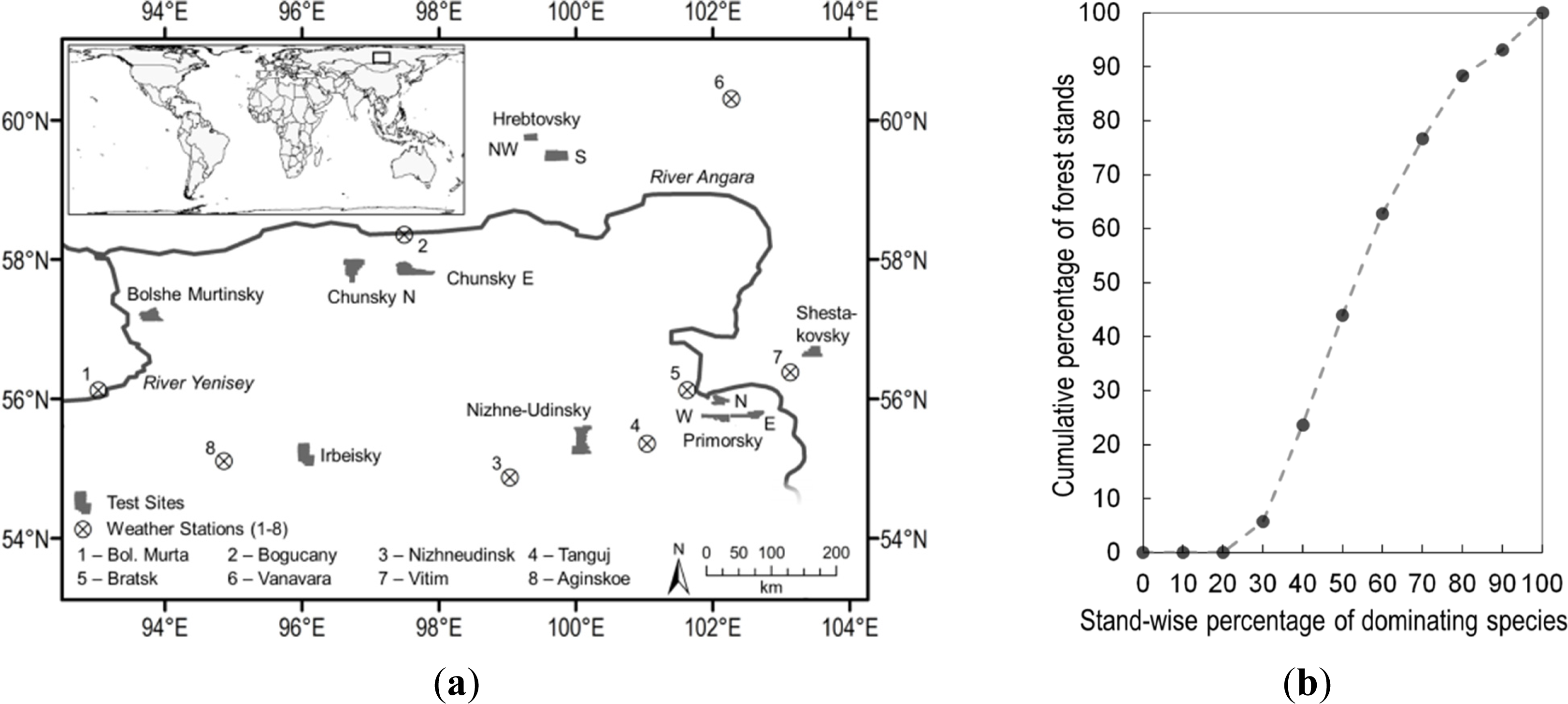
2.1. Study Area

The study area is located in Central Siberia, Russia and features parts of the administrative compartments Irkutsk Oblast and Krasnoyarsk Kray. It is placed in the so called Middle Siberian Plateau (see Figure 1a). The area is characterized by hills up to 1,700 m in the southern part. The northern part is rather flat with elevations up to 500 m. Taiga forests dominate and cover approximately 80% of the region. The region exhibits extreme continental climatic conditions. The yearly amount of precipitation is generally below 450 mm. Most of the precipitation occurs in summer. Winters are very cold and dry, while summers are warm and also feature long dry periods. The whole territory is characterized by forest cover disturbances caused by forest fires, insect outbreaks and logging.

2.2. Forest Inventory Data

Russian National Forest Inventory (NFI) data was used for the sites Bolshe Murtinsky NE, Chunsky N and E, Primorsky N, E, and W, Hrebtovsky S, and NW, Nishni Udinsky, Irbeisky and Shestakovsky (see Figure 1a and

Table 1. Forest characteristics of local sites according to National Forest Inventory (NFI) data (av = average, med = median, std = standard deviation, min = minimum, max = maximum).

Local Site	Size (km2)	No. of Stands	GSV (m3·ha−1) (av/med/std/min/max)	Dominant Species (Fraction ≥ 10%)
Bolshe NE	278	1,604	167/190/108/0/450	Fir (31%), Aspen (23%), Birch (15%), Spruce (10%)
Chunsky E	381	1,113	115/90/115/0/430	Birch (29%), Pine (24%), Larch (17%)
Chunsky N	393	1,284	129/150/112/0/470	Pine (21%), Birch (19%), Larch (16%), Spruce (11%)
Hrebtovsky NW	105	339	191/200/70/0/320	Pine (45%), Larch (37%)
Hrebtovsky S	287	867	171/190/90/0/420	Larch (40%), Pine (26%), Birch (13%)
Nishne Udinsky	514	2,046	169/190/124/0/470	Birch (41%), Pine (31%), Aspen (12%)
Irbeisky	400	1,720	165/190/111/0/500	Fir (28%), Birch (19%), Cedar (13%), Aspen (12%)
Primorsky E	209	994	152/180/113/0/500	Pine (34%), Birch (27%)
Primorsky N	149	752	119/90/98/0/350	Pine (44%), Aspen (22%), Birch (22%)
Primorsky W	180	710	137/120/100/0/440	Birch (36%), Pine (34%)
Shestakovsky	201	814	183/210/97/0/380	Pine (26%), Birch (24%), Larch (17%), Aspen (12%)

). Each of the sites comprises more than 300 stands. The forest inventory data contains a multitude of parameters including stand number, GSV (in 10 m³ ha⁻¹ classes), relative stocking, and the stand-wise canopy proportion of dominating species. Typically, Siberian forest is unmanaged. Therefore, the majority of the stands are covered with more than one tree species (Figure 1b). The average stand size is approximately 25 ha. Excluding clear-cuts the average GSV is 180 m³·ha⁻¹ which corresponds to a tree height of 18 m.

NFI determined the GSV from stem diameter at breast height (DBH) and tree height measurements [19] using tree species-specific allometric relationships. Typically, in boreal forests these allometric relationships are rather similar for the different tree species. Based on the available data it was estimated that the average forest stand tree height h_v is correlated with GSV across all species (GSV = 20.9e^0.11hv, R² = 0.76). Furthermore, a strong correlation was found between average stand DBH and h_v (h_v = 0.65 DBH^1.2, R² = 0.96). Note that the GSV of the inventory data were provided in classes of 10 m³/ha—clear-cuts are represented featuring a GSV of 0 m³/ha. The data were on hand digitally in vector format.

In accordance to Russian forest inventory standards, the accuracy of the provided GSV lies between 15% and 20% relative root mean square error (RMSE) [2]. Due to the Russian inventory standards, some specific characteristics of the forestry data base had to be considered: (i) Only trees with economic relevance are included (DBH > 6 cm, etc.); (ii) forest stands can be partly logged; (iii) the polygons are often inaccurate—the misregistration partially amounts 100 m; (iv) the last update of the inventory data was accomplished about 9 yr before the PALSAR acquisitions. Thus, new clear-cuts, fire scars, insect damages, growth, and regrowth of forest are disregarded. To overcome most of these problems, the following steps were applied: (i) Buffering polygons, to avoid errors caused by misregistration; (ii) excluding forest stands being partly/entirely logged, burned or destroyed by insect outbreaks since the last update of the inventory data by using recent high spatial resolution KOMPSat (Korea Multi-Purpose Satellite) and TerraSAR-X satellite data; (iii) excluding forest stands < 2 ha.

2.3. Meteorological Data

In Siberia the network of meteorological stations is sparse. The distance between the forest inventory data sites and the corresponding meteorological station can be greater than 200 km. Accordingly, the precipitation data needs to be interpreted with care. In particular during summer, when thunderstorm-type precipitation is prevalent, the measurements at the stations are not necessarily related to the precipitation at the test sites. For this reason and due to the low amount of precipitation it was decided to not exclude interferograms being potentially affected by rain.

Meteorological data were collected for the stations Bolshaja Murta, Bogucany, Nizhneudinsk, Tanguj, Bratsk, Vanavara, Aginskoe and Vitim (see Figure 1a). All meteorological data were gathered from the global World Meteorological Organization (WMO) weather station network. Temperature, precipitation, wind, and snow depth were gathered for the acquisition date of the SAR data. Regarding precipitation, the sum of the past 3 and 7 days prior to the acquisition was collected. This allows some inference on the soil and canopy moisture conditions. In almost all cases, during the winter (roughly November to March), the temperatures were below freezing. During summer/autumn (roughly June to October), the temperatures were above 0 °C. Thus, in general, frozen conditions can be assigned to winter and non-frozen conditions to summer acquisitions. Thaw was defined as when the minimum temperature was above freezing. SAR data acquired during thaw events were omitted in this work. At no time was heavy rain reported during the acquisitions. The maximum amount of precipitation was 8 mm (for one day). For most acquisition dates there was no precipitation. The measured wind speed was mostly close to zero.

2.4. PALSAR Data

Table 2. Employed Phased Array type L-band SAR (PALSAR) data. Italics: fine beam single polarization (FBS) (frozen conditions); Bold: fine beam dual polarization (FBD) (unfrozen conditions). Only image pairs from consecutive cycles were employed for interferogram processing, resulting in a total of 36 interferograms.

	Chunsky N	Chunsky E	Primorsky	Bolshe NE	Shesta-Kovsky	Nishne Udinsky	Irbeisky	Hrebtov-Sky
Track	T475	T473	T466	T481	T0463	T0471	T0478	T0468
Frame	F1150	F1150	F1110	F1140	F1130	F1100	F1100	F1190
2006		30 Dec		28 Dec
2007	20 Jun	14 Feb	18 Jan	12 Feb	13 Jan	11 Jan		6 Jan
	5 Aug	2 July	5 Mar	15 Aug	28 Feb	26 Feb		21 Feb
	20 Sep	17 Aug	21 Jul	30 Sep	16 Jul	14 Jul		9 Jul
	5 Nov	2 Oct	5 Sep		31 Aug	14 Oct		24 Aug
	21 Dec		21 Oct	31 Dec			26 Dec	9 Oct
2008	5 Feb	2 Jan		15 Feb	16 Jan		10 Feb	9 Jan
	22 Mar	17 Feb			2 Mar		28 Dec	24 Feb
2009		4 Jan		2 Jan	18 Jan	16 Jan	12 Feb	11 Jan
		19 Feb		17 Feb	5 Mar	3 Mar	30 Jun	26 Feb
					21 Jul		15 Aug	14 Jul
					5 Sep		30 Sep	29 Aug
								14 Oct
No. inter-ferograms	5	5	3	4	5	3	4	7

summarizes the employed PALSAR data. According to the PALSAR acquisition strategy [20], fine beam single polarization (FBS) data (HH) were acquired in winter (roughly November to March), and beam dual polarization (FBD) data (HH, HV) were acquired in summer/autumn (roughly June to October). Altogether, 64 single look complex (SLC) images were used in this study (FBS: 38 images, FBD: 26 images). Only HH polarization was used. The azimuth pixel spacing of the SLC data is 3.15 m. The slant range pixel spacing is 4.7 m for FBS (28 MHz), and 9.4 m for FBD (14 MHz) data. Regarding interferogram processing, only image pairs from consecutive cycles (46-day temporal baseline) were employed, resulting in a total of 36 interferograms. The perpendicular baseline B_⊥ varied between 50 m and 700 m for FBD data (acquired at unfrozen conditions) and between 50 m and 1,700 m for FBS data (acquired during frozen conditions). The impact of B_⊥ on volumetric decorrelation was studied within the ranges above for sparse and dense forest. Only minor effects were detected, temporal decorrelation dominated (see [4]).

3. Methodology

3.1. Coherence Data Processing and Approach of Investigation

INSAR requires two complex SAR images, S₁ and S₂, usually acquired from two slightly different positions. The distance between the sensor positions is called the baseline and the perpendicular component B_⊥ determines the sensitivity for volume decorrelation. The complex interferogram of S₁ and S₂, is formed by applying Equation (1), where S^* is the complex conjugate of S and 〈·〉 denotes ensemble average using an estimation window.

$$\gamma =\frac{\langle S_1{S}_2^{*}\rangle }{\sqrt{\langle {\left|S_1\right|}^2\rangle }\langle {\left|S_2\right|}^2\rangle }$$

(1)

The parameter γ is the complex correlation between S₁ and S₂ and consists of a phase and a magnitude (|γ|) component. The magnitude varies between 1 and 0, with 1 perfect and 0 refers to no correlation.

Interferometric processing consisted of single look complex (SLC) data co-registration at the sub-pixel level [21,22], slope adaptive common-band filtering in range [22,23], and common-band filtering in azimuth. The interferograms were generated using 10 × 20 looks for fine beam single polarization (FBS) data and 10 × 40 looks for fine beam dual polarization (FBD) data. For FBD the number of azimuth looks was doubled to gather approximately squared pixels in ground range geometry, accepting the trade-off of lower geometric resolution. The dissimilar number of independent looks results in a slight difference of the coherence estimation bias and thus the zero-coherence bias (of 0.03) [24,25]. The zero-coherence bias was estimated by processing normally distributed random data, resulting in a |γ| of 0.07 for the FBD and of 0.10 for the FBS processing chain. The |γ| images were orthorectified using Shuttle Radar Topography Mission (SRTM) elevation data.

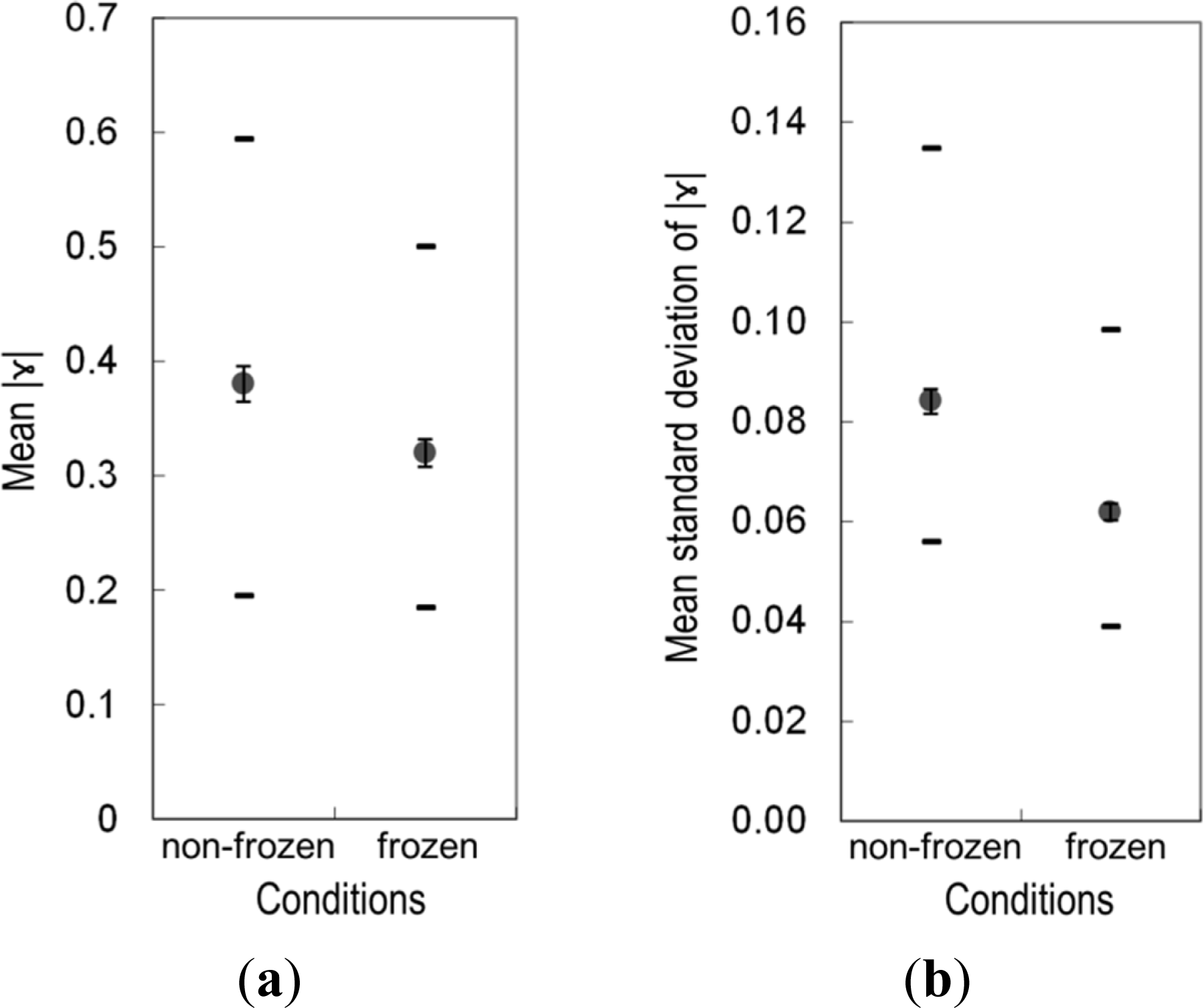
3.2. Statistical Analysis of |γ|

All analyses were conducted on forest stand level. Thus, |γ| was averaged for each forest stand. Only those forest stands were considered where the dominating tree species covered at least 80%. This selection represents roughly 10% of the 12,243 stands. The choice of a higher percentage would have resulted in the loss of almost all stands and was thus not feasible (see Figure 1b).

The survey of the impact of species on coherence was focused on dense forest to reduce ground contribution of the signal and pronounce the impact of trees. Dense forest refers to GSV from 200 m³·ha⁻¹ to 300 m³·ha⁻¹. The average GSV of the stands was close to 250 m³·ha⁻¹ for all species. Saturation for GSV using L-band coherence in Siberia commonly occurs at GSV < 200 m³·ha⁻¹ [2,4]. Thus, GSV variations within the defined GSV range of dense forest are assumed to have negligible effects on |γ|. Considering all sites, approximately 2,000 dense forest samples are available, while one sample refers to one forest stand covered by one interferogram. The trees species composition of dense forest, and thus the partitioning of samples was as follows: 31.7% pine, 19.3% fir, 17.9% larch, 11.7% birch, 10.2% aspen, 6.9% spruce, and 2.4% cedar. Due to the low amount of samples spruce and cedar could not be considered. To summarize the experimental results, several descriptive statistics have been computed:

(i)

Average and standard error of |γ| of all stands with dense forest (250–350 m³·ha⁻¹);

(ii)

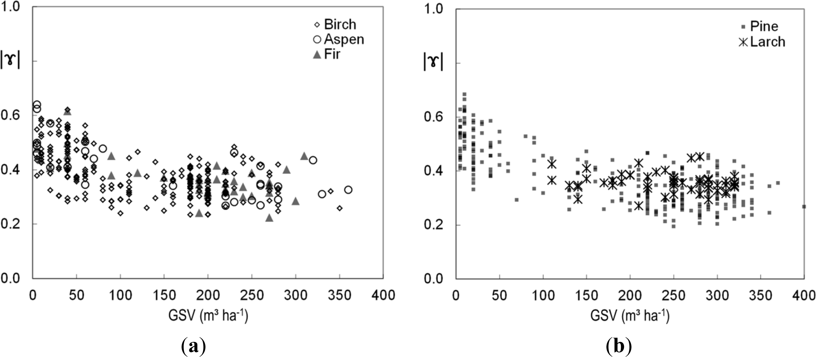
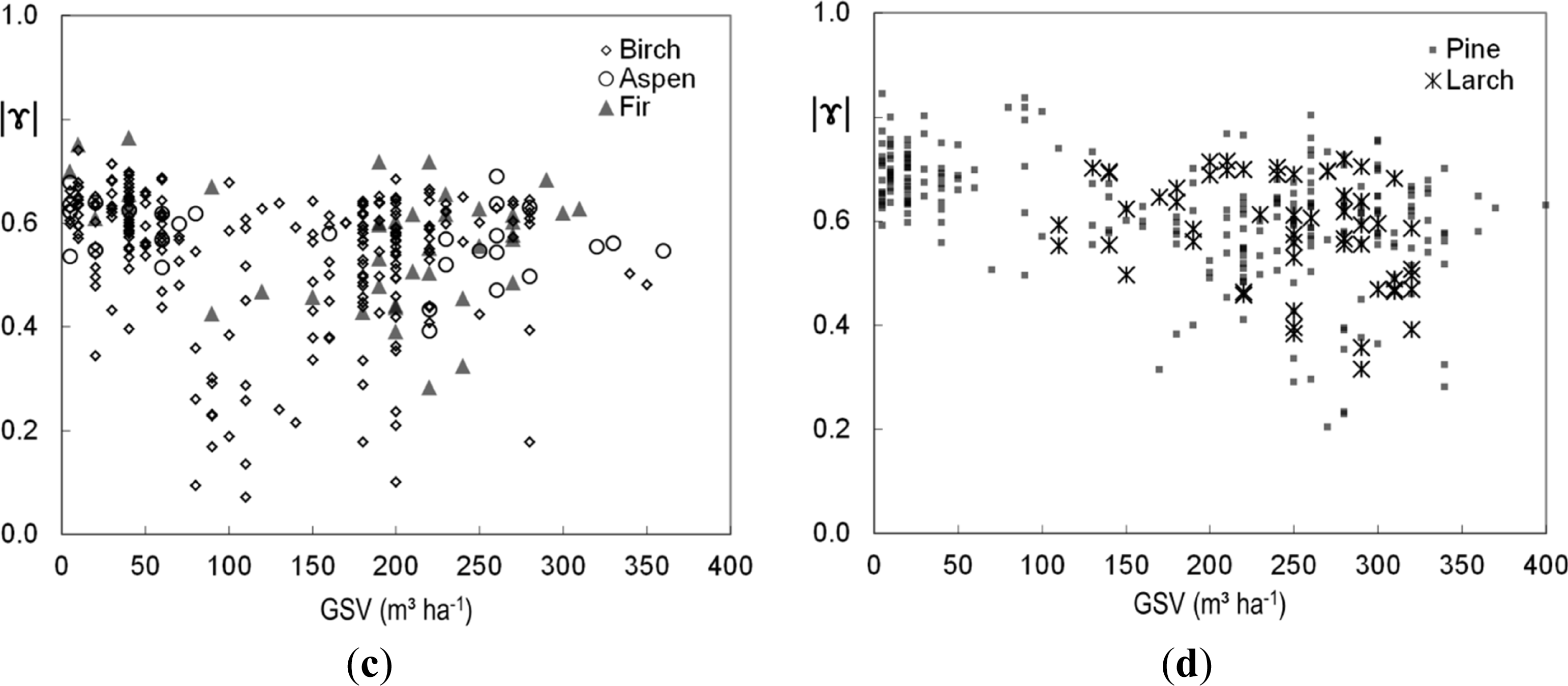
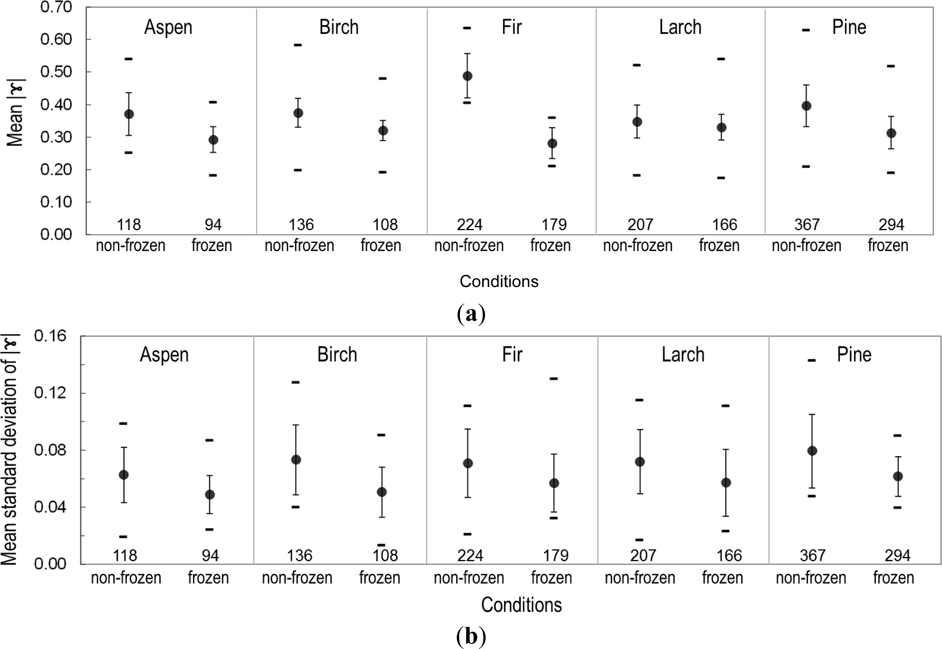
Average and standard deviation of |γ| separated by species;

(iii)

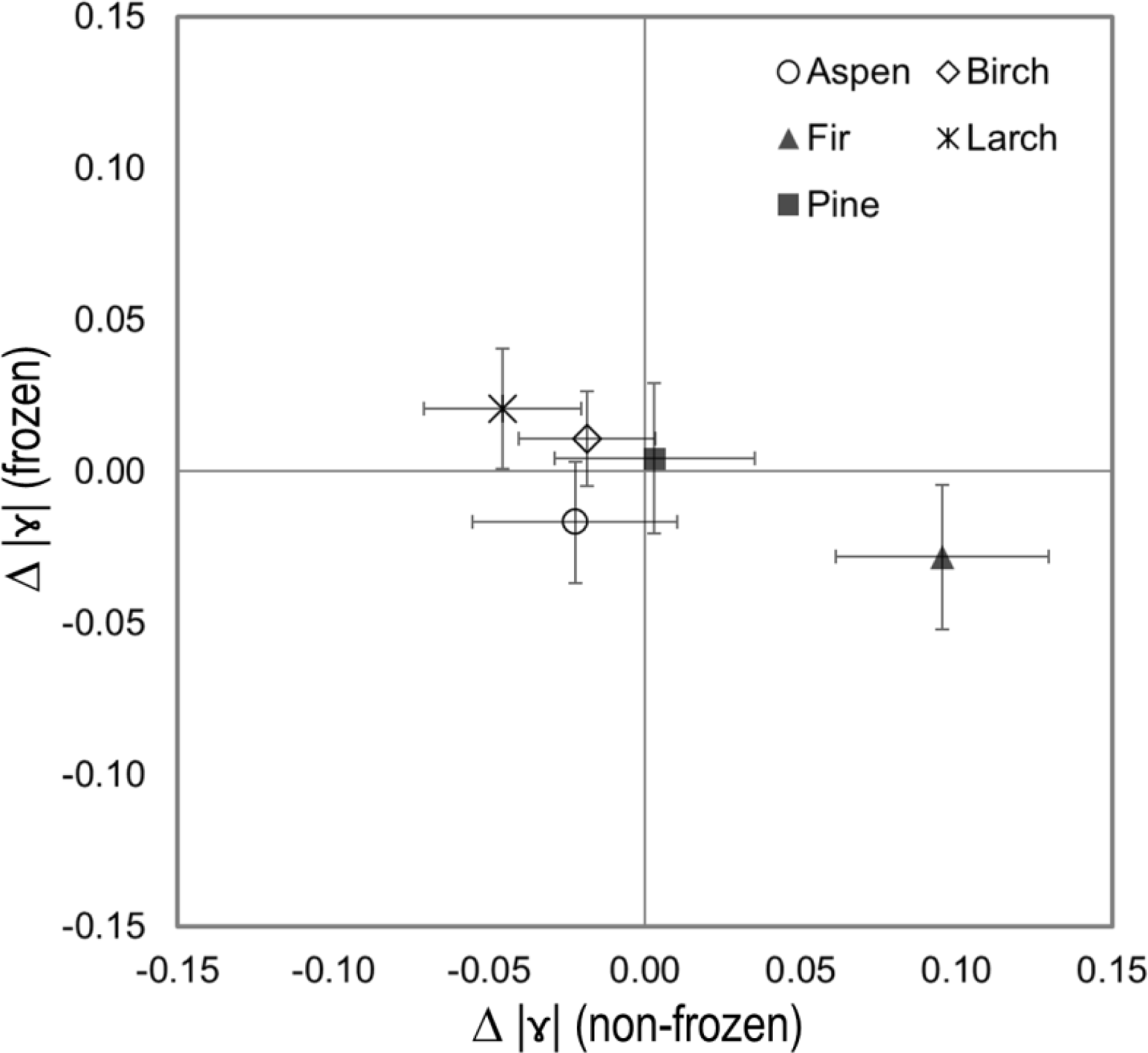
Deviation of tree species specific |γ| from average |γ| over dense forest;

(iv)

T-tests to evaluate significance of difference.

All results are separated by frozen and unfrozen conditions.

4. Results and Discussion

The observed standard deviation of |γ| over dense forest is higher under non-frozen conditions (see Figure 2b), which is in accordance with former studies [2,4] based on Japanese Earth Resources Satellite (JERS-1) and PALSAR data. Furthermore, it was observed that the average of |γ| of dense forest is significantly higher (confidence > 99.5%) under non-frozen conditions. The significance was evaluated applying the t-test resulting in a t-value of 3.3. This value is greater than the 0.995-quantile of the t-distribution: t(0.995; 70) = 2.648. This issue of increased |γ| during unfrozen conditions was thoroughly analyzed in [4]. It was suggested that the deeper penetration of the incoming SAR signal results in increased volume decorrelation. Furthermore, the observations revealed increased temporal decorrelation over dense forest during frozen state.

Figure 3a–d provides a typical example of a PALSAR based GSV-|γ| scatterplot (do not consider the symbols for the species at this time). Under frozen conditions (Figure 3a,b), an increment of GSV results in decreasing |γ|. Under unfrozen conditions (Figure 3c,d), this trend is hardly visible. This is partly due to the spread of |γ| at all GSV levels. One potential reason for this spread is the spatiotemporal variability of environmental conditions during the growing season. Soil moisture and vegetation conditions can vary spatially resulting in variable temporal decorrelation for the same GSV level. In winter, however, trees and soil are frozen, and little variation occurs in moisture. Precipitation in the form of very dry snow does not cause significant spatial differences of temporal decorrelation for L-band data [6,9,26]. Another potential reason for the dissimilar observations between unfrozen and frozen conditions is related to forest structure and tree species. During unfrozen state, differing tree species and forest structure can be accompanied by varied temporal decorrelation. Geometric properties, such as crown shape or alignment of tree components, affect attenuation and the distribution of the major scatterers, and thus volumetric decorrelation [11–13].

During winter, under frozen and calm conditions, tree species-specific temporal decorrelation is unlikely. Geometric properties are also of less importance. Due to freezing the dielectric constant of the trees is reduced [7,27], resulting in decreased attenuation and a reduced InSAR phase height above the ground [5]. Thus, the amount of scattering within the canopy is also decreased [8] and the shape and structure of the canopy has less impact on the backscattered signal.

For the sake of clarity the data set shown in Figure 3 was split into two groups. Under frozen conditions (Figure 3a,b) all tree species follow the same trend and no obvious deviations occur. Under non-frozen conditions (Figure 3c,d), differences between the species are apparent. For instance the coherence of birch and pine is much more scattered than that of spruce or aspen. Additionally, birch features by far the lowest minimum coherence. Nevertheless, from Figure 3 no specific trend for the tree species can be observed. In Figure 3 the overall spread of |γ| is not caused by differences between species, but by the variations within the species. This observation, however, considers only one site and one interferogram.

Figure 4 summarizes species specific mean and standard deviations of |γ| for dense forest based on all sites and interferograms. During non-frozen conditions all species feature higher coherence variability than under frozen conditions. Also, the species specific |γ| are more diverse at unfrozen state (see also Figure 5). The standard deviation of |γ| is roughly 0.02 larger under non-frozen condition for all species. This finding is most likely caused by increased spatiotemporal variability of the environmental conditions during non-frozen conditions, as discussed above.

Figure 5 depicts the average deviation (difference) of the tree species specific |γ| from the average |γ| of dense forest for frozen and non-frozen conditions considering all sites and interferograms. Thus, it combines the information of Figures 2a and 4a to summarize the observations. Under frozen conditions the deviation is rather small and reaches roughly +0.02 for larch and −0.03 for fir. Nevertheless, due to the low coherence level at frozen state this deviation is statistical significant (t-test, confidence > 95%). For the other species the mean deviations are much smaller. For example, the signatures of pine and birch do observably overlap. The confidence (t-test) that both species cause dissimilar |γ| is < 60%. During non-frozen conditions, the deviation is increased and reaches values of up to +0.10 for fir and −0.05 for larch. In other words, during non-frozen conditions the |γ| of fir is 0.15 greater than the |γ| of larch, which is a significant difference (t-test, confidence > 99%). Thus, a clear impact on |γ| is observable for some tree species under non-frozen conditions.

5. Conclusions

The impact of the tree species on |γ| of dense Siberian forest was observed to be small in average, when frozen conditions are considered (in accordance to [14] and [18]). For non-frozen conditions the impact is increased against frozen conditions. Deciduous species (aspen, birch, larch) exhibit the lowest |γ| (in accordance to [15]). This impact of tree species on |γ| under non-frozen conditions causes a fraction of the observed spread of the GSV-coherence relationship (when the trend is investigated across all species). Thus, temporal and/or volumetric decorrelation to some extent depend on the characteristics of the specific species.

Moreover, increased intra-species variance of |γ| was observed for non-frozen conditions compared to frozen conditions. Assuming similar geometric properties of the trees of one species, the amount of geometric decorrelation should not differ much between the stands, as all stands feature dense forest. The large spread of coherence can rather be explained by varying temporal decorrelation caused by spatiotemporal variable environmental conditions as described above. Under frozen conditions, however, environmental conditions are much more stable in space and time resulting in decreased spread of |γ|. By all means, choosing SAR data acquired under frozen conditions is preferable when aiming at coherence based GSV assessment across species. When only data acquired under non-frozen conditions is available, the impact of the species on |γ| needs to be considered.

References

1. Koskinen, J.T.; Pulliainen, J.T.; Hyyppä, J.M.; Engdahl, M.E.; Hallikainen, M.T. The seasonal behavior of interferometric coherence in boreal forest. IEEE Trans. Geosci. Remote Sens 2001, 39, 820–829. [Google Scholar]
2. Eriksson, L.E.B.; Santoro, M.; Wiesmann, A.; Schmullius, C.C. Multitemporal JERS repeat-pass coherence for growing-stock volume estimation of Siberian forest. IEEE Trans. Geosci. Remote Sens 2003, 41, 1561–1570. [Google Scholar]
3. Pulliainen, J.; Engdahl, M.; Hallikainen, M. Feasibility of multi-temporal interferometric SAR data for stand-level estimation of boreal forest stem volume. Remote Sens. Environ 2003, 85, 397–409. [Google Scholar]
4. Thiel, C.; Schmullius, C. Investigating ALOS PALSAR interferometric coherence in central Siberia at unfrozen and frozen conditions: implications for forest growing stock volume estimation. Can. J. Remote Sens 2013, 39, 232–250. [Google Scholar]
5. Thiel, C.; Schmullius, C. Investigating the impact of freezing on the ALOS PALSAR InSAR phase over Siberian forests. Remote Sens. Lett 2013, 4, 900–909. [Google Scholar]
6. Santoro, M.; Fransson, J.E.S.; Eriksson, L.E.B.; Magnusson, M.; Ulander, L.M.H.; Olsson, H. Signatures of ALOS PALSAR L-band backscatter in Swedish forest. IEEE Trans. Geosci. Remote Sens 2009, 47, 4001–4019. [Google Scholar]
7. Dobson, M.G.; McDonald, K.; Ulaby, F.T. Effects of Temperature on Radar Backscatter from Boreal Forests. Proceedings of the 1990 IEEE International Geoscience and Remote Sensing Symposium (IGARSS), College Park, MD, USA, 20–24 May 1990; pp. 2481–2484.
8. Kwok, R.; Rignot, E.J.M.; Way, J.; Freeman, A.; Holt, J. Polarization signatures of frozen and thawed forests of varying environmental state. IEEE Trans. Geosci. Remote Sens 1994, 32, 371–381. [Google Scholar]
9. Eriksson, L.E.B.; Schmullius, C.C.; Wiesmann, A. Temporal Decorrelation of Spaceborne L-Band Repeat-Pass Coherence. Proceedings of the Parameters from SAR Data for Land Applications BioGeoSAR, Innsbruck, Austria, 16–19 November 2004. (CD-ROM).
10. Santoro, M.; Askne, J.; Smith, G.; Fransson, J.E.S. Stem volume retrieval in boreal forests from ERS-1/2 interferometry. Remote Sens. Environ 2002, 81, 19–35. [Google Scholar]
11. Hyyppä, J.; Hallikainen, M. Applicability of airborne profiling radar to forest inventory. Remote Sens. Environ 1996, 57, 39–57. [Google Scholar]
12. Solberg, S.; Astrup, R.; Gobakken, T.; Næsset, E.; Weydahl, D.J. Estimating spruce and pine biomass with interferometric X-band SAR. Remote Sens. Environ 2010, 114, 2353–2360. [Google Scholar]
13. Izzawati; Wallington, E.D.; Woodhouse, I.H. Forest height retrieval from commercial X-band SAR products. IEEE Trans. Geosci. Remote Sens 2006, 44, 863–870. [Google Scholar]
14. Santoro, M.; Shvidenko, A.; McCallum, I.; Askne, J.; Schmullius, C. Properties of ERS-1/2 coherence in the Siberian boreal forest and implications for stem volume retrieval. Remote Sens. Environ 2007, 106, 154–172. [Google Scholar]
15. Castel, T.; Martinez, J.M.; Beaudoin, A.; Wegmuller, U.; Strozzi, T. ERS INSAR data for remote sensing hilly forested areas. Remote Sens. Environ 2000, 73, 73–86. [Google Scholar]
16. Askne, J.; Santoro, M. Multitemporal repeat pass SAR interferometry of boreal forests. IEEE Trans. Geosci. Remote Sens 2005, 43, 1219–1228. [Google Scholar]
17. Proisy, C.; Mougin, E.; Lopes, A.; Sarti, F.; Dufrêne, E.; Ledantec, V. Temporal Variations of Interferometric Coherence over a Deciduous Forest. Proceedings of the SAR Workshop: CEOS Committee on Earth Observation Satellites, Toulouse, France, 26–29 October 1999; p. 25.
18. Wagner, W.; Luckman, A.; Vietmeier, J.; Tansey, K.; Balzter, H.; Schmullius, C.; Davidson, M.; Gaveau, D.; Gluck, M.; Toan, T.L.; et al. Large-scale mapping of boreal forest in SIBERIA using ERS tandem coherence and JERS backscatter data. Remote Sens. Environ 2003, 85, 125–144. [Google Scholar]
19. National Forest Inventory (NFI). National Forest Inventory Guidelines (In Russian); Russian Federation: Moscow, Russia, 2009; Volume 1. [Google Scholar]
20. Rosenqvist, A.; Shimada, M.; Ito, N.; Watanabe, M. ALOS PALSAR: A pathfinder mission for global-scale monitoring of the environment. IEEE Trans. Geosci. Remote Sens 2007, 45, 3307–3316. [Google Scholar]
21. Wegmüller, U. Automated and Precise Image Registration Procedures. Proceedings of the 1st International Workshop on Multitemp, Trento, Italy, 13–14 September 2001; pp. 37–49.
22. Wegmüller, U. SAR Interferometric and Differential Interferometric Processing. Proceedings of the IEEE International Geoscience and Remote Sensing Symposium (IGARSS), Seattle, WA, USA, 6–10 July 1998; pp. 1106–1108.
23. Santoro, M.; Werner, C.; Wegmüller, U.; Cartus, O. Improvement of Interferometric SAR Coherence Estimates by Slope-Adaptive Range Common Band Filtering. Proceedings of the IEEE International Geoscience and Remote Sensing Symposium (IGARSS), Barcelona, Spain, 23–28 July 2007; pp. 129–132.
24. Touzi, R.; Lopes, A.; Bruniquel, J.; Vachon, P.W. Coherence estimation for SAR imagery. IEEE Trans. Geosci. Remote Sens 1999, 37, 135–149. [Google Scholar]
25. López-Martínez, C.; Pottier, E. Coherence estimation in synthetic aperture radar data based on speckle noise modeling. Appl. Opt 2007, 46, 544–558. [Google Scholar]
26. Rott, H.; Nagler, T.; Scheiber, R. Snow Mass Retrieval by Means of Sar Interferometry; European Space Agency-European Space Research Institute (ESA-ESRIN): Rome, Italy, 2003.
27. Way, J.; Rignot, E.J.M.; Mcdonald, K.C.; Oren, R.; Kwok, R.; Bonan, G.; Dobson, M.C.; Viereck, L.A.; Roth, J.E. Evaluating the type and state of Alaska taiga forests with imaging radar for use in ecosystem models. IEEE Trans. Geosci. Remote Sens 1994, 32, 353–370. [Google Scholar]
Figure 1. (a) Map of the study area. Each of the test sites comprises more than 300 stands. Excluding clear-cuts the average growing stock volume (GSV) is 180 m3·ha−1 which corresponds to a tree height of 18 m; (b) Stand-wise canopy proportion of dominating species vs. cumulative proportion of all available stands (in total: 12,243). A stand-wise percentage of the dominating species of 100 means pure stands, a percentage of 80 means that the dominating species covers 80% of the forest stand area. At approximately 90% of the stands the canopy proportion of the dominating tree species is smaller than 80%.
Remotesensing 06 01124f1
Figure 2. Mean (a) and standard deviation (b) of |γ| for dense forest (200–300 m3·ha−1)—all sites. Symbols: average (•), standard error (⊥ ⊤), minimum/maximum (–). Mean and standard deviation are higher for non-frozen conditions. The displayed values are based on all 36 interferograms. Each of the 36 |γ| images is one sample in this population (unfrozen: 20 images, frozen: 16 images).
Remotesensing 06 01124f2
Figure 3. |γ| vs. GSV by dominant tree species for Primorsky South using two single interferograms. (a) and (b): Frozen conditions (18 January 2007–5 March 2007); (c) and (d): Non-frozen conditions (21 July 2007–5 September 2007).
Remotesensing 06 01124f3aRemotesensing 06 01124f3b
Figure 4. Mean (a) and standard deviation (b) of |γ| over dense forest (200–300 m3·ha−1) by dominant tree species and environmental conditions—all sites. Symbols: average (•), standard deviation (⊥ ⊤), minimum/maximum (–). The figures at the bottom lines of the diagrams represent the numbers of samples.
Remotesensing 06 01124f4
Figure 5. Deviation Δ of tree species specific |γ| from average |γ| of dense forest for frozen and non-frozen conditions—all sites. The average |γ| of dense forest is shown in Figure 2a.
Remotesensing 06 01124f5