Segmentation-Based Filtering of Airborne LiDAR Point Clouds by Progressive Densification of Terrain Segments

Abstract

Filtering is one of the core post-processing steps for Airborne Laser Scanning (ALS) point clouds. A segmentation-based filtering (SBF) method is proposed herein. This method is composed of three key steps: point cloud segmentation, multiple echoes analysis, and iterative judgment. Moreover, the third step is our main contribution. Particularly, the iterative judgment is based on the framework of the classic progressive TIN (triangular irregular network) densification (PTD) method, but with basic processing unit being a segment rather than a single point. Seven benchmark datasets provided by ISPRS Working Group III/3 are utilized to test the SBF algorithm and the classic PTD method. Experimental results suggest that, compared with the PTD method, the SBF approach is capable of preserving discontinuities of landscapes and removing the lower parts of large objects attached on the ground surface. As a result, the SBF approach is able to reduce omission errors and total errors by 18.26% and 11.47% respectively, which would significantly decrease the cost of manual operation required in post-processing.

1. Introduction

Airborne LiDAR (Light Detection and Ranging), also termed Airborne Laser Scanning (ALS), is now a widely employed technology to capture the 3D geometry of the Earth ground surface and the objects on it [1]. Currently, ALS has various types of applications, ranging from the reconstruction of digital terrain models (DTM; [2,3]), 3D building models [4–7] and 3D road models [8] to the detection of individual tree crowns [9,10], measurement of tree height and estimation of other forest stand parameters [11,12], hydraulic applications [13,14], power lines reconstruction, infrastructure mapping [15], etc. In most ALS applications, filtering is a necessary step to determine which LiDAR returns are from the ground surface and which are from the off-terrain objects [16].

An experimental comparison of the performance of eight filter algorithms was presented by Sithole and Vosselman [17]. They concluded that, surface-based filters often yield better results concerning the filter strategy, because they use more context than other filter strategies. Among surface-based filtering methods, progressive TIN (triangular irregular network) densification (PTD) is widely employed in both the scientific community and engineering applications, because it has been integrated into the commercial software TerraSolid. However, discontinuities in the bare ground (see Figure 1a) and low objects attached on the ground surface (see Figure 1c) also pose great challenges to the classic PTD method. It often fails to detect the terrain points on break lines and step edges, and mistakes the lower parts of objects as ground ones, as shown in Figure 1b,d respectively.

To overcome the above shortcomings, Tóvári and Pfeifer [18] proposed a segmentation-based robust interpolation filter based on the method of Kraus and Pfeifer [19]. They first segmented the raw point clouds, and then, the residuals were computed for each segment instead of each point. Depending on the residual, all points in one segment are assigned to a same weight in robust interpolation. The experiments in [18] suggested that combination of segmentation-based approach and surface-based approach is promising and robust in both urban and forested areas, which may attribute to the following three factors:

(1)

After point cloud segmentation, segments are capable of reaching exactly up to the break lines or jump edges;

(2)

An explicit surface model can be used. Describing the expected terrain surface with a dedicated model allows including terrain characterization in the filter process [18];

(3)

The surface-based approach is useful in the wooded areas.

To conclude, although many methods have been developed to tackle the filtering problem, it has not been fully solved so far. However, Hutton and Brazier [14] emphasized that errors in filtering and interpolation will affect subsequent use – for example using terrain in a hydraulic model, or vegetation height estimation in biomass calculation. In this article, we propose a segmentation-based filtering (SBF) approach (see Section 3), which combines a point cloud segmentation method and the classic PTD’s framework. The first step of our filtering approach is point cloud segmentation for the point cloud (see Section 3.2). In the second step, an analysis of multiple echoes is performed to remove the vegetation measurements (see Section 3.3). At last, segments are classified either as ground or object segments based on the principles of the classic PDT method (see Section 3.1). However, the main difference between our method and the classic PDT method is that a segment instead of a single point is the basic processing unit.

2. Previous Work

Lots of filtering methods have been proposed so far. According to the filter concept, Sithole and Vosselman [17] separated existing filtering methods into four classes, i.e., slope-based, surface-based, clustering/segmentation, and block-minimum algorithms; and this category is still feasible today. Among them, the first three classes of filtering methods are more popular, and they are surveyed as follows.

(1)

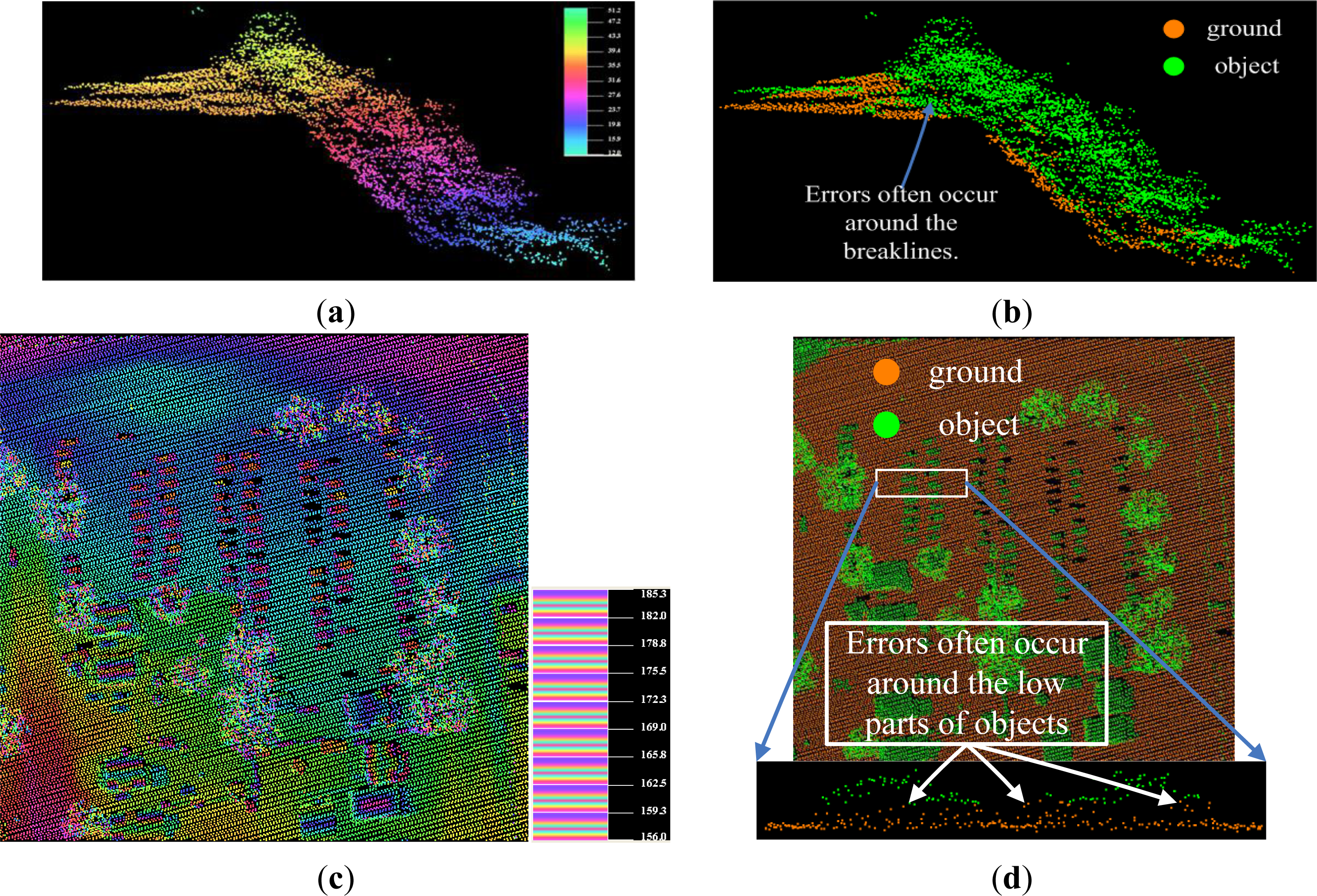
In slope-based approaches, the slope or height difference between two points is measured. The rationale behind these algorithms is that the steepest slopes in a landscape belong to objects and the terrain has a certain maximum slope. Thus, if the slope is above a certain threshold then the highest point is assumed to belong to an off-terrain object. Vosselman did the pioneering work [20] about slope-based filtering. Some extensions and variants of slope-based filters focus on the shape of structure elements [21], the determination of adaptive slope parameters [22], and topological analysis removing very large buildings [10]. The slope-based methods usually work well when object and terrain points are equally mixed. However, typical filter errors are encountered when this requirement is not met.

(2)

In surface-based approaches, the basic idea is to create a parametric surface with a corresponding buffer zone above it, the surface locates the buffer zone, and as before the buffer zone defines a region in 3D space where ground points are expected to reside [17]. Thus, the core step of this kind of methods is to create a surface approximating the bare earth [23]. Depending on the means of creating the surface, surface-based filtering methods can be further divided into three subcategories: morphology-based filters [23,24], iterative-interpolation-based filters [19,25,26], and progressive-densification-based filters [27]. Axelsson [27] first divided the whole point dataset into tiles, and then selected the lowest points in each block as the initial ground points, and finally a TIN of the identified ground points was constructed as the reference surface. For each triangle, one additional ground point was determined by investigating the parameters of the unclassified points in each triangle with the reference surface. The parameters were the distance to the TIN facets and the angles to the nodes. If a point was found with offsets below the threshold values, it was classified as a ground point and the algorithm proceeds with the next triangle. Before continuing with the next iteration, all ground points were added to the TIN. In this way, the triangulation was progressively densified until all points were classified as ground or object. Axelsson’s method is known as PTD [3,17]. The above surface-based approaches are preferred in engineering applications [28].

(3)

In segmentation-based approaches, it is commonly assumed that segments of objects are situated higher than the ground segments. Generally, segment-based filters generally consist of two steps, the first one being segmentation and the second one being filtering based on the generated segments. Lohmann [29] applied the compactness of these segments and the height difference to the neighboring segments in order to detect different types of areas. Lee [30] first obtained planar patches from the points with a region growing method, and then these patches are grouped into a set of surface clusters. It is assumed that the connected and continuous surface patches belong to the same object and that large vertical discontinuities usually do not exist between ground segments. The ground clusters are selected on the basis of a simple assumption that objects are above the ground and ground clusters are relatively large. Sithole and Vosselman [31] compared the neighboring segment heights in different directions and predefined a set of rules, finally each segment was classified as object or ground. Shen et al. [32] assumed that the ground segments are horizontal and lower than the adjacent object segments. Yan et al. [33] also presented an object-based filtering method. The above segment-based filters are typically designed for urban areas where many step edges can be found in the data. A shortcoming of these filters is that there is no intended terrain model as done in the in the above surface-based approaches. Additionally, too many small segments may be generated in forested areas, which will challenge the existing filters.

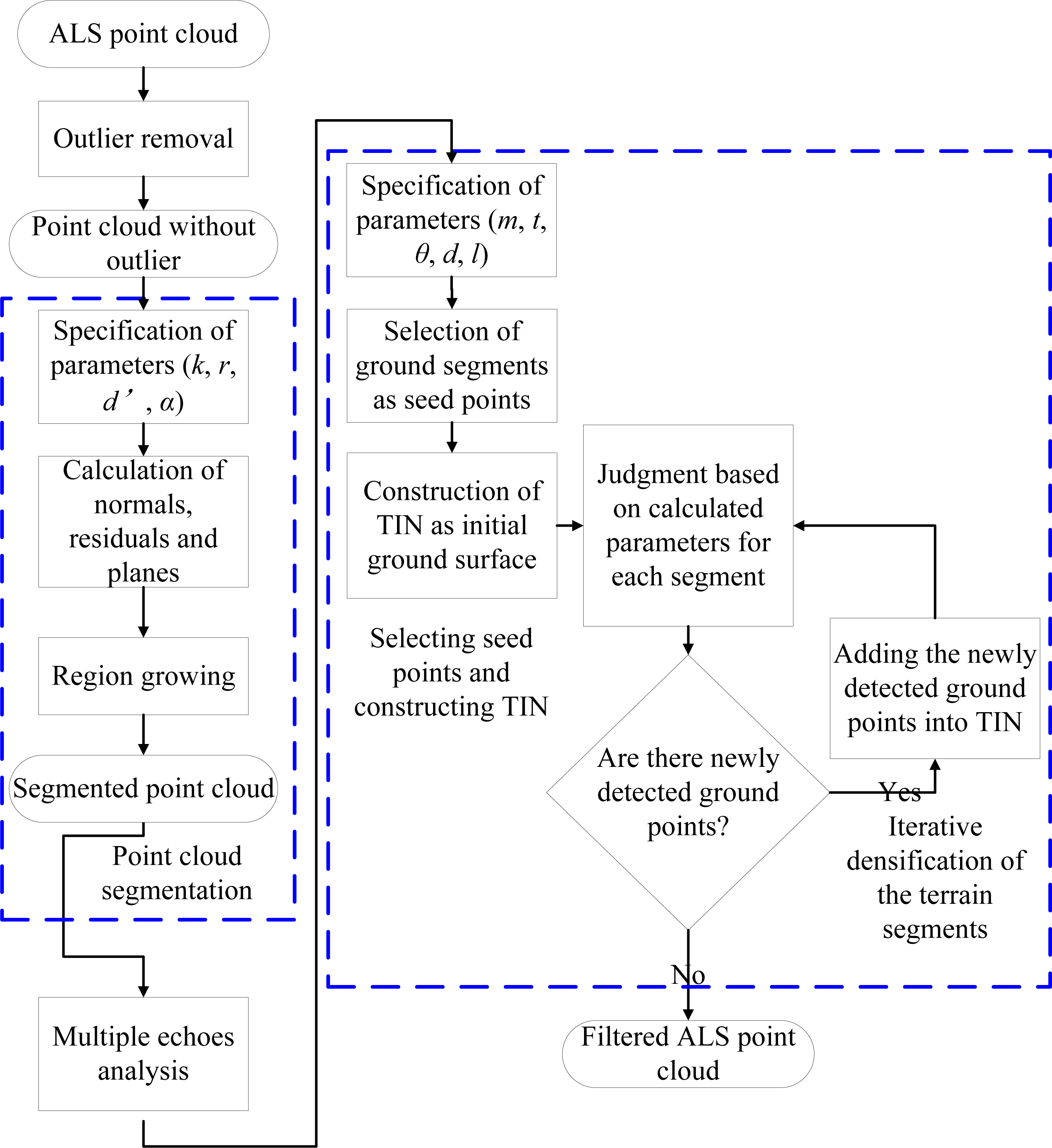
The proposed SBF approach is a combination of the surface-based PTD method and the segmentation-based method. Our goal is to integrate the strengths of both methods to increase the filtering accuracy.

3. Method

The proposed SBF method is composed of four steps: outlier removal (see Section 3.1), point cloud segmentation (see Section 3.2), multiple echo information analysis (see Section 3.3), and progressive densification of the terrain segments (see Section 3.4), as shown in Figure 2.

3.1. Outlier Removal

Many datasets contain measurements that are far above or below the earth surfaces, and these measurements are called outliers. Outlier is one of the circumstances under which the filter algorithms are likely to fail [17], especially for the filters based on the assumption that the lowest point in a grid cell must belong to the terrain [3]. Our SBF approach is also sensitive to the outliers, especially the low outliers. However, automatic outlier removal is an impossible mission, because there are various types of errors, such as low outliers, high outliers, isolated outliers, and clustered outliers. Thus, human participation is needed. Herein, three sub-steps are designed to eliminate the outliers. Firstly, an elevation histogram is built and examined by visualizing the distribution of elevation values, and then elevation thresholds were determined by the human operator’s visual evaluation to eliminate the lowest and highest tails from the distribution. Secondly, the remaining outliers were searched using the minimum height difference of each point with respect to all its neighbors. Herein, a kd tree [34] is employed to query the neighbors of each point, and the average elevation and standard deviation of the elevations are calculated. Points, that are higher or lower three times of the standard deviation to the average elevation, are removed from the dataset. Thirdly, errors yielded by the automatic outlier classification are corrected manually.

3.2. Point Cloud Segmentation

Practices suggest the processing of LiDAR data can be strengthened by first segmenting the point clouds and then analyzing segments rather than individual points [35]. Point cloud segmentation is the process to partition an input point cloud into coherent and connected point clusters [36]. Specifically, points on a certain geometric feature are coherent points, such as coplane, co-surface, and coline points; whilst connected points are a group of points in which every point has at least one neighboring point within a certain distance [37]. There are many airborne LiDAR point cloud segmentation methods, such as region-growing [38], surface growing [39], and adaptive random sample consensus [40]. However, most of them aim at detecting the planar surfaces (such as building roofs) rather than the smooth surfaces (such as ground surfaces in large areas). Herein, Tóvári and Pfeifer’s segmentation method [18] is employed. This segmentation method is based on the assumption that, continuous and smooth surfaces could be clustered into the same segments. We rename it as point cloud smooth segmentation (PCSS) method. PCSS is composed of the following two main stages.

(1)

Normal and residual estimation. The normal for each point is estimated by fitting a plane to the neighboring points. Therefore, k nearest neighbors (KNN) [34] is employed for the neighborhood search. To fit a plane to a set of given points, in a least squares sense, we need to find the parameters that minimize the sum of squares of the orthogonal distances of the points from the estimated surface. The best-fitting plane is calculated using the principal component analysis (PCA), which is derived from the theory of the least-squares estimation. PCA is a popular method for computing plane normal approximations from point clouds, and the details of plane fitting refer to Rabbani [41].

(2)

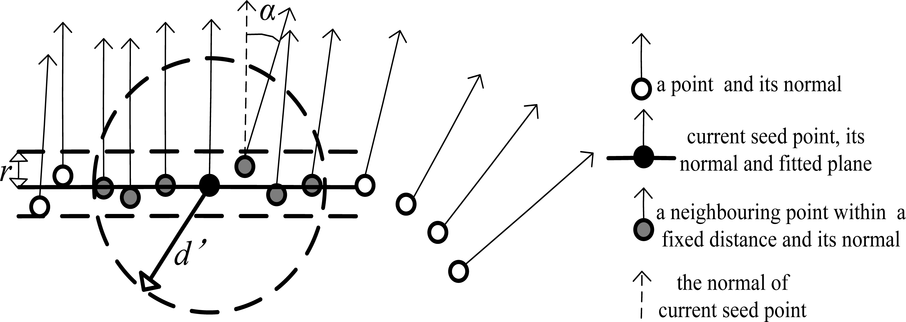
Region growing with distance and normal difference constraint. This stage makes use of the above calculated normals, in accordance with user specified parameters to cluster points belonging to smooth surfaces. The process of region growing proceeds in the following steps:

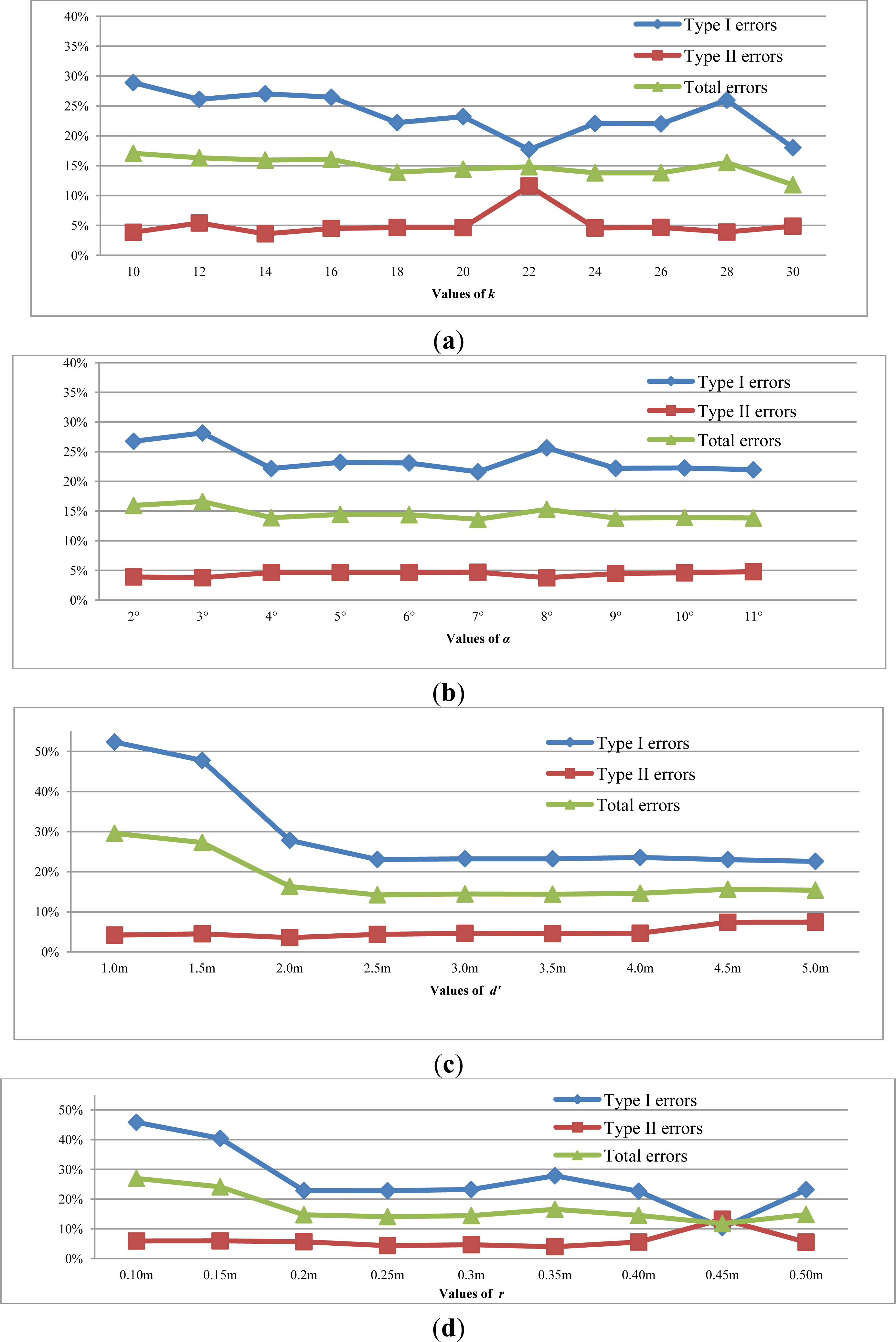
• ① Input two smoothness thresholds in terms of the distance. The first threshold is the normal distance of a neighboring point to the current plane, denoted as r. The second threshold is the 3D distance between the current point and a neighboring point, denoted as d'.
• ② Input a smoothness threshold in terms of the angle between the normals of the current seed and its neighbors, denoted as α. Set all point to un-segmented.
• ③ If all the points have already been segmented, go to step ⑦. Otherwise, select the point with minimum residual from unlabeled points as the current seed, and build an empty list of seed points.
• ④ Select the fixed distance neighboring points of the current seed. Fixed distance neighbors (FDN) is used to search the neighboring points within a fixed distance d'. Add the points, whose angle difference to current seed is less than α and whose distance to the current plane is less than r, to current region; simultaneously, add the qualified points to the list of potential seed points.
• ⑤ If the potential seed point list is not empty, set the current seed to the next available seed and current plane to the next available seed’s plane, and go to step ④.
• ⑥ Add the current region to the segmentation and go to step ③, and clear the list of seed points. Note that the residuals of the labeled points should be excluded when the point with minimum residual is searched.
• ⑦ Finish the task of segmentation.

The above PCSS algorithm needs four specified parameters, k, r, d', and α (see Figure 3). These parameters should be determined based on experience and the complexity of the landscapes. Some examples of PCSS are displayed in Figures 4b, 5c and 6c. The figures show that, after segmentation, the ground surface is grouped into many dominant clusters, and the objects are also grouped into many clusters. Moreover, most of the clusters contain a clear majority of either ground or object points, whereas there are hardly any mixed clusters. Particularly, despite the terrain clusters being crossed by breaklines, terrain clusters may contain points on both sides of slope discontinuities.

3.3. Multiple Echo Information Analysis

Currently, the multi-pulse airborne LiDAR system is capable of recording both single returns/echoes and multiple returns [42]. Practice suggests that the proportion of the multiple returns in each segment is a good feature to distinguish vegetation measurements from ground measurements [10,32,43,44]. As mentioned above, the vegetation is likely to produce multiple echoes. Experiments suggest that segments belonging to trees contain few points in which the multiple returns occupy a proportion more than 50% [43], as shown in Figures 5d and 6d. Simultaneously, the segments belongings to buildings contain a large number of points in which singular returns occupy a proportion more than 90% [44]. Echo ratio is also employed for vegetation classification in full-waveform airborne LiDAR data [45]. Therefore, the feature about proportion of multiple echoes is also informative. Thus, if the proportion of multiple echoes in a segment is larger 50%, the points within the segment are labeled as vegetation class and they are forbidden to take partition the subsequent judgment.

3.4. Progressive Densification of the Terrain Segments

This step is similar to the progress of the PTD filter, but the basic processing unit is a segment rather than a single point (as shown in Figure 4c).

It is composed of the following five steps.

(1)

Specifying parameters. There are five key parameters [3] to be preset, including:

• ① Maximum building size, m. m is a length threshold, and the algorithm can deal with buildings having a length of up to this value. It is used to define the grid cell size, and a grid cell is a tile of the point cloud (see the step (2)).
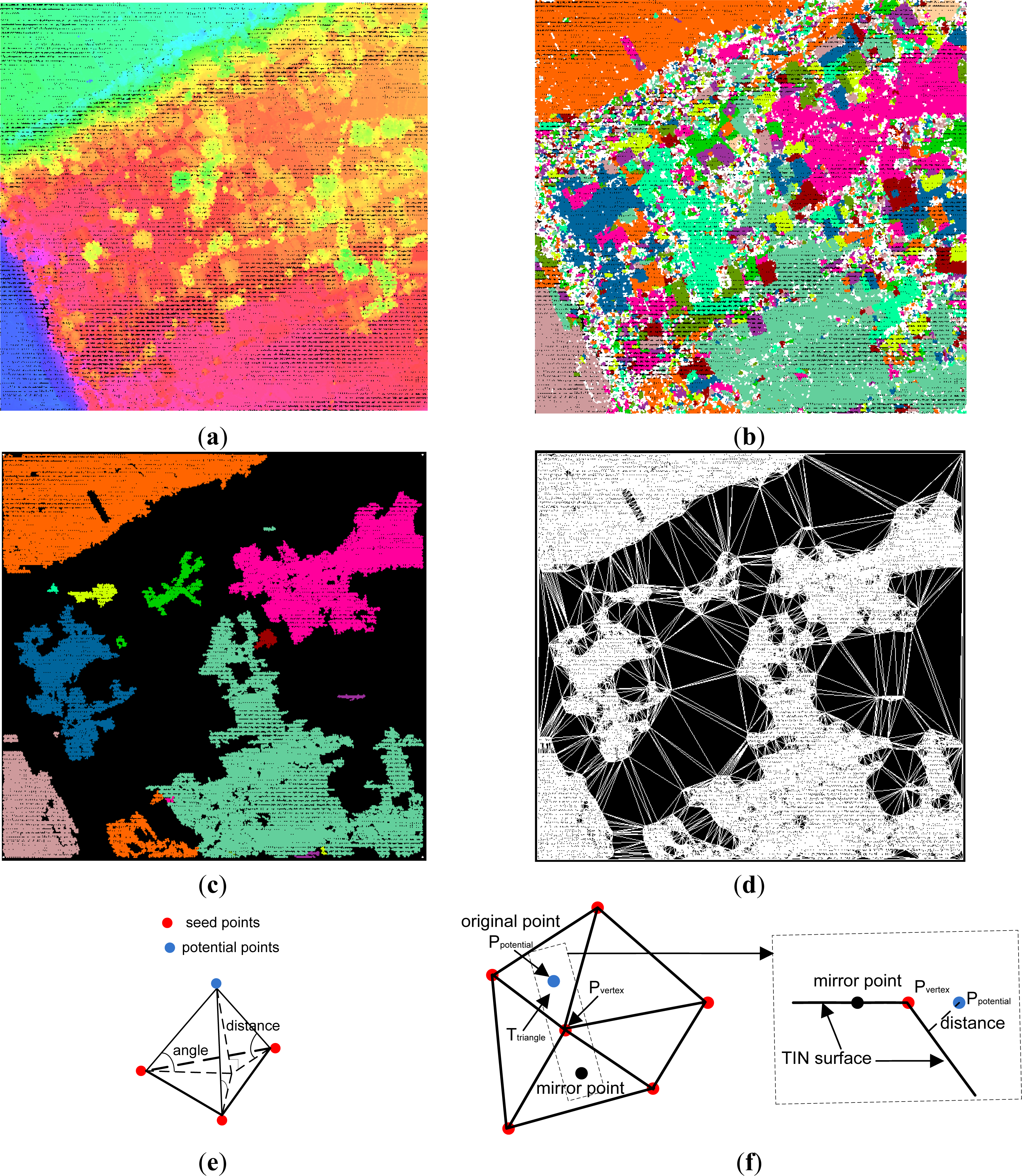
• ② Maximum terrain angle, t. t is a slope threshold, which decides how the judgment of an unclassified point is performed (either mirroring or not). If the slope of a triangle in the TIN is larger than t, any unclassified/potential point located inside of this triangle should be judged by a corresponding mirror point. The mirroring idea is from [27]. More details are presented in the step (3)-④, illustrated in Figure 4f.
• ③ Maximum angle, θ. θ is the maximum angle between a triangle plane and a line connecting a potential point with the closest triangle vertex. If an unclassified point has a larger angle than θ, it is labeled as an object measurement, otherwise as a ground measurement.
• ④ Maximum distance, d. d is the maximum orthogonal distance from a point to triangle plane during one iteration. If an unclassified point has a larger distance than d, it is labeled as an object measurement, otherwise as a ground measurement.
• ⑤ Minimum edge length, l. l is the minimum threshold for the maximum (horizontally projected) edge length of any triangle in the TIN. l is utilized to reduce the eagerness to add new points to the ground inside a triangle when every edge of a triangle is shorter than l. Note that l is measured in the horizontal plane. Thus, introduction of l helps to avoid adding unnecessary points to the ground model and reduces memory requirements.

Note that the classic PTD filter also needs presetting the same five parameters.

(2)

Selecting seed terrain segments and constructing initial TIN

Determine the bounding box of the given point cloud dataset, and fix the top left corner (x_topleft, y_topleft), bottom right corner (x_bottomright, y_tbottomright), width w and height h. The whole region of dataset is divided into several tiles (or grid cells) in rows and columns. Number of rows and columns are determined by the following formula:

$$n_{\text{Row}}=\mathit{ceil}\left(\frac{h}{m}\right) \text{and} n_{\text{Column}}=\mathit{ceil}\left(\frac{w}{m}\right)$$

(1)

where n_Row is the number of tiles in rows, n_Column is the number of tiles in columns, m is the above parameter about maximum building size, ceil(x) is a function used to return the smallest integral value that is not less than x. The segment with the lowest point in each tile is regarded as a terrain segment, and the points belonging to the terrain segments are selected as seed points of the dataset. Note that there is no repeating in the seed points. This means, if the lowest points in several tiles belong to the same segment, the points belonging to the same segment should be added into the seed points only once, as shown in Figure 4c,d. Additionally, the four corners on the bounding box should be added to the seed points, as shown in Figure 4c,d. Moreover, each corner’s height is equal to its closest seed point on horizontal plane. At last, a TIN is constructed based on the seed points, as shown in Figure 4d, and it represents an initial terrain model. Note the insertion of the four corners guarantees that any point in the point cloud dataset is located inside the TIN. After the TIN is constructed, the remaining points, except the seed points, are labeled as default object measurements.

(3)

Labeling

Judging is performed in a segment-wise style. In other words, the potential points belonging to the same segment are judged as a whole. In detail, set all segments except the terrain ones in an unprocessed state. Find an unprocessed segment, and the points within the segment labeled as object measurements. Subsequently, make a judgment of each potential point in the segment as follows:

• ① Locate the potential point, P_potential(x_p, y_p, z_p). Find the triangle, T_triangle, which the P_potential is inside or on the edge of or on the vertex of.
• ② Calculate the slope of the triangle plane, S_triangle. If S_triangle is not larger than terrain angle t, go to ③. Otherwise, go to ④.
• ③ Calculate the following two parameters, A_angle and D_distance, as shown in Figure 4e. This first is the angle between T_triangle and a line connecting P_potential with the closest triangle vertex, denoted as A_angle. The second is the distance from P_potential to T_triangle, denoted as D_distance. If both of the following cases:

  • A_angle ≤ θ
  • D_distance ≤ d

  hold, label Ppotential as ground measurement, and go to judgment of the next point. Otherwise, go to next one.
• ④ Mirroring Ppotential, as shown in Figure 4f. Find the vertex with highest elevation value in Ttriangle, denoted as Pvertex(x_v, y_v, z_v). Ppotential is mirrored as follows:

  $$\begin{array}{c}{x}_{\text{mirror}}=2x_{\text{v}}-x_{\text{P}}\\ y_{\text{mirror}}=2y_{\text{v}}-y_{\text{P}}\\ z_{\text{mirror}}=z_{\text{P}}\end{array}$$

  (2)

  where (x_mirror, y_mirror, z_mirror) are the 3D coordinates of the mirror point. Locate the mirror point, and calculate the angle and distance parameters as done in ③. If the mirror point is determined as a ground point, label P_potential as ground measurement, and go to judgment of next point.

If all points within the current segment have been judged, set the segment in a processed state, and count the number of the ground points and the number of the object points. If the number of ground measurements is larger than the object measurements, label all of the points within the current segment as ground measurement. Otherwise, label them as object measurements again, and go to judgment of next unprocessed segment. However, if all segments are processed and labeled, go to step (4).

(4)

The newly detected terrain segments are added into the TIN as follows:

• ① Locate the ground point, P_ground(x_g, y_g, z_g) in each terrain segment one by one. Find the triangle, T'_triangle, which the P_ground is inside or on the edge of or on the vertex of.
• ② Calculate the length of each edge of T'_triangle in horizontal plane. If the length of any edge is larger than l, add P_ground into the TIN. Otherwise, go to the judgment of the next newly detected ground point.

(5)

Repeat (3) and (4) until no further segment is added to the set of terrain segments anymore.

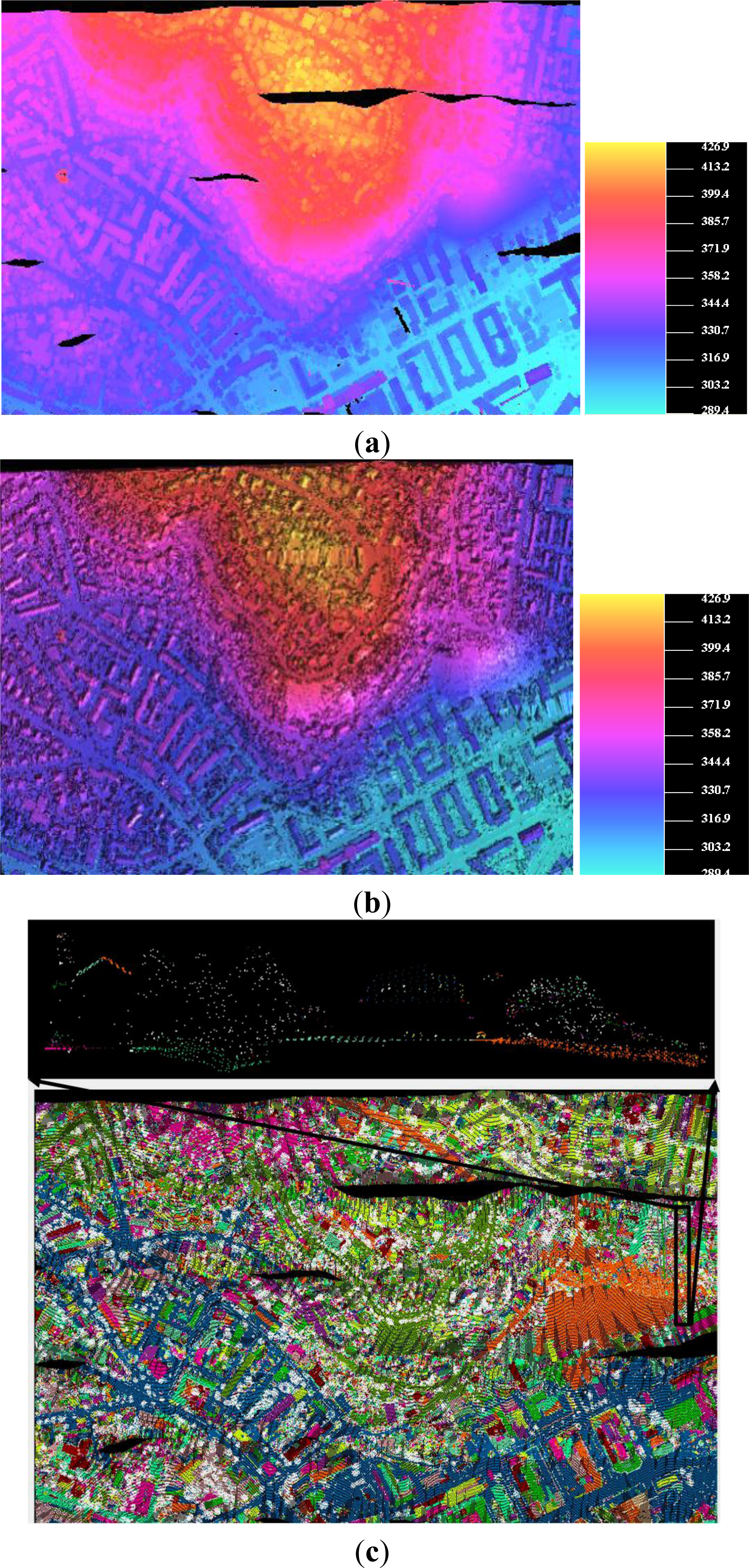
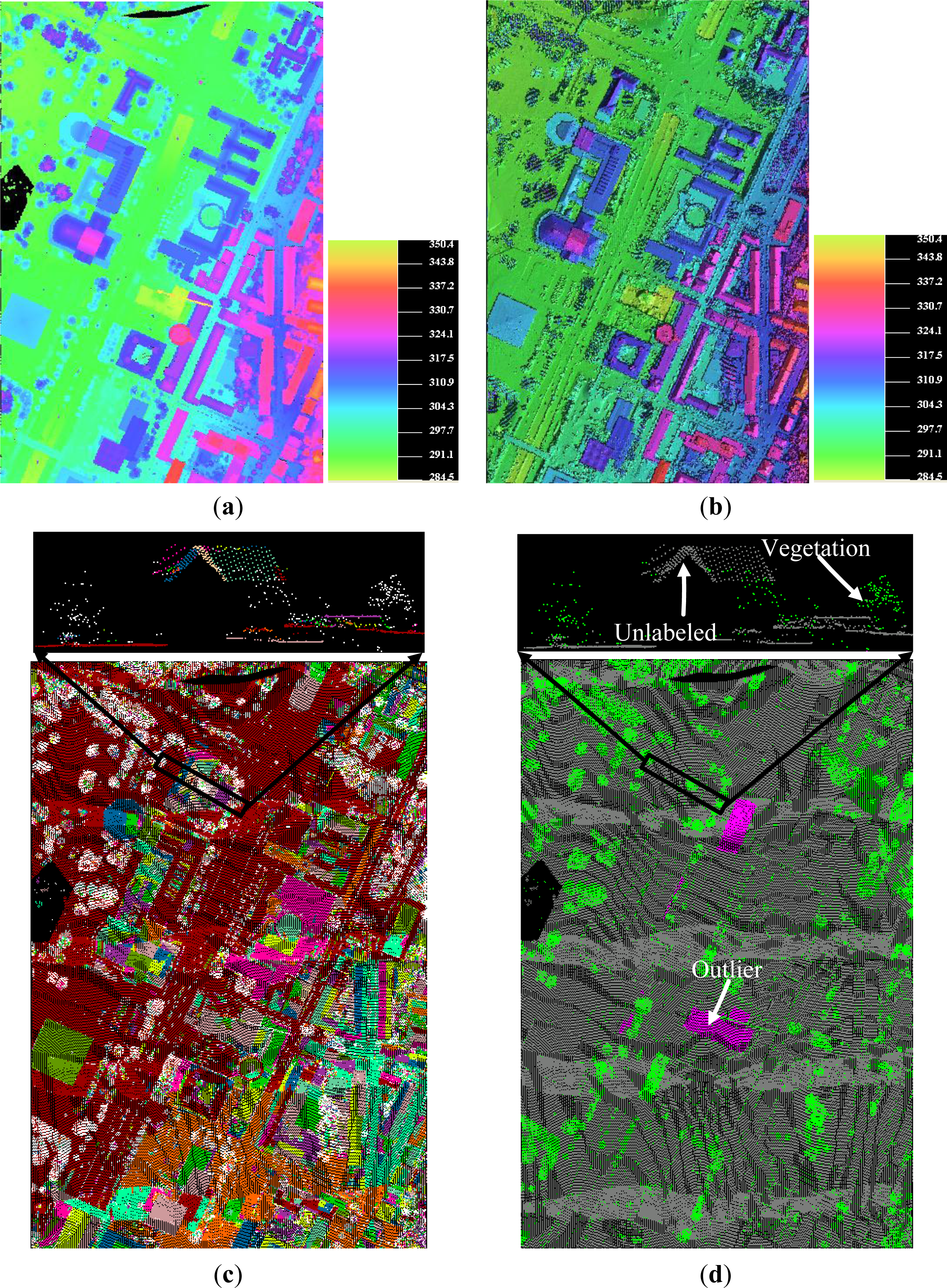
4. Experiments and Performance Evaluation

A prototype software system for filtering ALS data has been developed using VC++6.0 IDE under the Windows XP Operating System. The hardware we used is a Lenovo workstation W520, with an Intel Pentium 2.40 GHz CPU and 2.98 GB RAM. The classic PTD method [27], PCSS segmentation method [18], and the proposed SBF approach are integrated into the developed system. Note that we implemented the PTD and PCSS from scratch. Additionally, the triangulation of the ALS points was done by integrating an existing implementation of a 2D Delaunay triangulator called Triangle [46] and the KNN was done by integrating an existing implementation of kd tree called ANN [47].

4.1. Experimental Data

The benchmark data from ISPRS Commission III, Working Group III are employed to compare the performances of the PTD method and the proposed SBF method. It includes eight sites consisting of different terrains: four urban sites and four rural/wooded sites, as well as 15 reference samples of sub-areas. The eight datasets are named as CSite1-8, respectively, as listed in

Table 1. Input Parameters of the two filters used for each site.

Parameters	Classic PTD Method					SBF Method
Scene	m (m)	t (°)	θ(°)	d (m)	l (m)	k (points)	r (m)	d' (m)	α (°)
CSite1	20	80	6	1.4	1	20	0.3	3	10
CSite2	60	88	6	1.4	1	20	0.3	3	5
CSite3	35	88	6	1.4	1	20	0.3	3	10
CSite4	60	88	6	1.4	1	20	0.3	3	10
CSite5	10	70	6	1.0	2	20	0.3	3	15
CSite6	40	70	6	1.4	2	20	0.3	3	5
CSite7	20	70	6	1.4	2	20	0.3	3	10

. The test data cover various land-use and land-cover types including buildings, vegetation, rivers, roads, railroads, bridges, etc. These data were obtained by an Optech ALTM scanner over the Vaihingen/Enz test field and the Stuttgart city center. The overall characteristics of these eight datasets refer to Sithole and Vosselman [17]. The point spacing is 1.0 to 1.5 m for urban sites and 2.0 to 3.5 m for rural sites, respectively. Moreover, there are a total of 15 reference samples for testing the filtering accuracy; the reference data were generated by manual filtering with knowledge of the seven landscapes and available aerial images [17]. As the CSite8 does not have a reference dataset, it was excluded for further experiment and analysis. Note that the laser data were collected with both first and last echoes/returns, which does not mean there is no single return in the data. To perform multiple echoes analysis, the original two echoes of each pulse are labeled as single returns or multiple returns based on the following rules:

• If intensity values of the two echoes are not same, they are both labeled as multiple echoes;
• Otherwise, calculate the 3D distance of the two echoes:

  • ▪ If their distance is larger than an experienced threshold, 0.5 m, they are also labeled as multiple echoes;
  • ▪ Otherwise, they are both labeled as single echoes.

The above preprocessing not only preserves all points in the original data, but also adds more echo information into the data. Note that multiple echoes analysis is performed by the both filters. Particularly, if a point is labeled as a multiple echo and it is also the first echoes of the two, it is filtered out in the multiple echoes analysis for the PTD filter.

4.2. Specification of the Input Parameters

The SBF method shares five parameters with PTD method, but needs four parameters more than the PTD method. For the seven datasets, the shared five parameters are set to the same values for both of the filters, as shown in Table 1. All of the parameters are determined by the authors’ experienced judgment on the conditions of the landscape. Particularly, m is slightly larger than the maximum length or width of the buildings in this scene; t is the maximum terrain slope in this scene; θ and d are set to 6 and 1.4 in default respectively, and their optimal values can be determined by the trial and error method; l is slightly larger than the average point density of the point dataset, which is used to avoid too many triangles in the TIN.

Table 1 lists all of the parameters used for the seven testing data.

Table 2. Statistics about the filtered results of the two filters for each site.

Indicators	Total Number of Points (points)	Number of Outliers (points)	Classic PTD Method				SBF Method
Scene			O	S	G	Time Cost (s)	O	S	G	Time Cost (s)
CSite1	1,366,408	2,485	118,375	1,929	445,430	24.77	198,176	516,993	611,671	891.17
CSite2	486,800	7,088	30,005	74	161,562	7.83	43,860	235,493	253,587	128.70
CSite3	377,028	393	37,693	144	146,310	6.84	51,994	174,523	188,240	104.34
CSite4	518,060	2,609	33,135	76	182,140	8.94	45,748	16,984	241,026	78.46
CSite5	628,576	199	42,956	17,084	447,742	17.13	104,601	436,082	485,118	302.18
CSite6	551,698	2,222	18,106	972	375,519	12.52	45,107	293,497	443,170	78.81
CSite7	393,264	1,086	11,096	2,742	312,449	10.51	27,399	304,661	346,347	83.73

Notes: “O” is the abbreviation of “Number of detected object points by multiple echoes analysis (points)”, “S” is the abbreviation of “Number of seed points (points)”, and “G” is the abbreviation of “Number of ground points (points)”. Moreover, the time cost includes only the time spending on computing rather than the time spending on reading and writing.

lists some key statistics about the input seven datasets and their results, such as the number of raw points, the number of detected outliers, etc.

4.3. Results

With the specified parameters in Table 1, we perform the filtering on the seven datasets using the two methods. Some statistics about the filtering refer to Table 2. Among the filtering results, we select CSite1 and CSite2 as two representatives to make a demonstration, shown in Figures 5 and 6, respectively. Both of CSite1 and CSite2 are partially or fully covered in urban areas, and the top of the CSite1 contains a hill with complex natural landscape and man-made objects. Furthermore, results of Sample 11, Sample 24, Sample 51, Sample 53, Sample 71 and Sample 12 are also displayed to reflect the details of filtering, as shown in Figures 7 and 12 respectively.

CSite1 is an urban area, and its special features include steep slopes, mixture of vegetation and buildings on hillside, buildings on hillside, and data gaps. There are 1,366,408 points in the raw data. 2,485 points are identified as outliers and excluded from the remaining filtering process for both the filters, and the remaining data and the corresponding TIN are displayed in Figure 5a,b, respectively. In the filtering process of the PTD, 118,375 points are detected as object measurements by the multiple echoes analysis; 1,929 points are selected as ground seed points; finally, 445,430 points are classified as ground measurements (see Figure 5g). In the filtering process of the SBF method, 198,176 points are detected as object measurements by the multiple echoes analysis (see Figure 5d); 516,993 points are identified as ground measurements (see Figure 5e); finally, there are 611,671 measurements being classified as ground (see Figure 5f). The statistics of the two filters on CSite1 suggest that, the proposed SBF method is capable of removing 67% object measurements, detecting 26,785% ground seed points, preserving 37% ground measurements more than the PTD filter. The differences of Figure 5f,g are shown in Figure 5h. Figure 5h suggest that the main difference attributes to the ability of SBF method to preserve the potential ground measurements in areas with steep terrain, as shown in the rectangular regions in Figure 5f–h. Figure 5g shows that most of the ground points around steep areas are omitted, and the lower part of a road across the steep terrain is missed for the classic PTD (see Figure 7d). In contrast, Figure 5f,h show that the ground measurements around the same steep areas and the whole road are well preserved by SBF method.

CSite2 is also an urban area, and its special features include large buildings, irregularly shaped buildings, a road with a bridge and a small tunnel, plus some data gaps. There are 973,598 points in the raw data. 124 points are identified as outliers. The remaining data without outliers and its TIN are displayed in Figure 6a,b, respectively. In the filtering process of the PTD, 30,005 points are detected as object measurements by the multiple echoes analysis; 74 points are selected as ground seed points; finally, 161,562 points are detected as ground measurements (see Figure 6g). Similarly, in the filtering process of SBF method, 43,860 points are detected as object measurements by the multiple echoes analysis (see Figure 6d); 235,493 points are identified as ground measurements (see Figure 6e); finally, there are 253,587 measurements being detected as ground (see Figure 6f). The statistics of the two filters on CSite2 suggest that, SBF proposed method is capable of removing 46% object measurements, detecting 326,974% ground seed points, preserving 57% ground measurements more than the PTD filter. The differences of Figure 6f,g are shown in Figure 6h. The reason of the difference between the two results is SBF method’s ability to preserve the ground measurement on some steep streets, as shown in the rectangular regions in Figure 6f–h. Figure 6g shows some road segments are omitted for the classic PTD. In contrast, Figure 6f shows all of the roads are well preserved by SBF method.

Additionally, the detailed results from the references of Sample 11, Sample 24, Sample 51, Sample 53 and Sample 71, suggest that SBF method can correctly detect more ground measurements than the PTD method in the case of:

• vegetation and buildings on steep slopes (see Figure 7);
• ramps in urban areas (see Figure 8);
• vegetation on slopes (see Figure 9);
• discontinuity caused by natural break lines(see Figure 10);
• discontinuity caused by bridges (see Figure 11) or highways.

Moreover, the SBF method is also capable of removing more small objects such as cars than the PTD method, as shown in the ellipse region in Figure 12. After the point cloud segmentation, the points corresponding to the same vehicle often belong to the same segment, and most of the points in the segment are judged as the non-ground class. Thus, the vehicle segment and all of the points in the segment are labeled as the non-ground class. There are many cars in Sample 12 [17], and Figure 12a,b display the filtered results of the PTD and the SBF method on the Sample 12, respectively. Compared with the PTD, less car measurements are remained in the result of SBF method. However, the SBF method fails to identify the off-terrain object measurements under the following conditions:

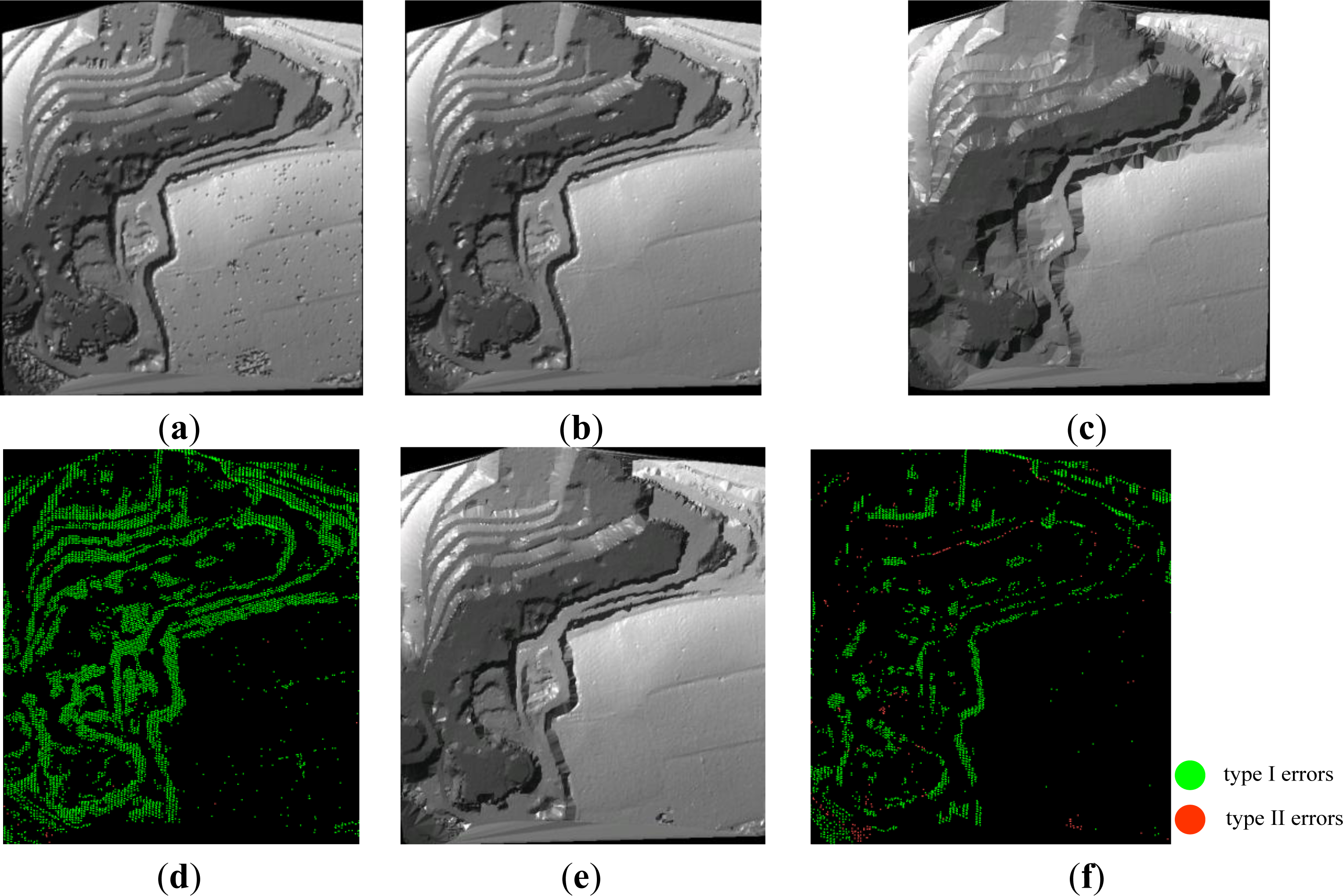
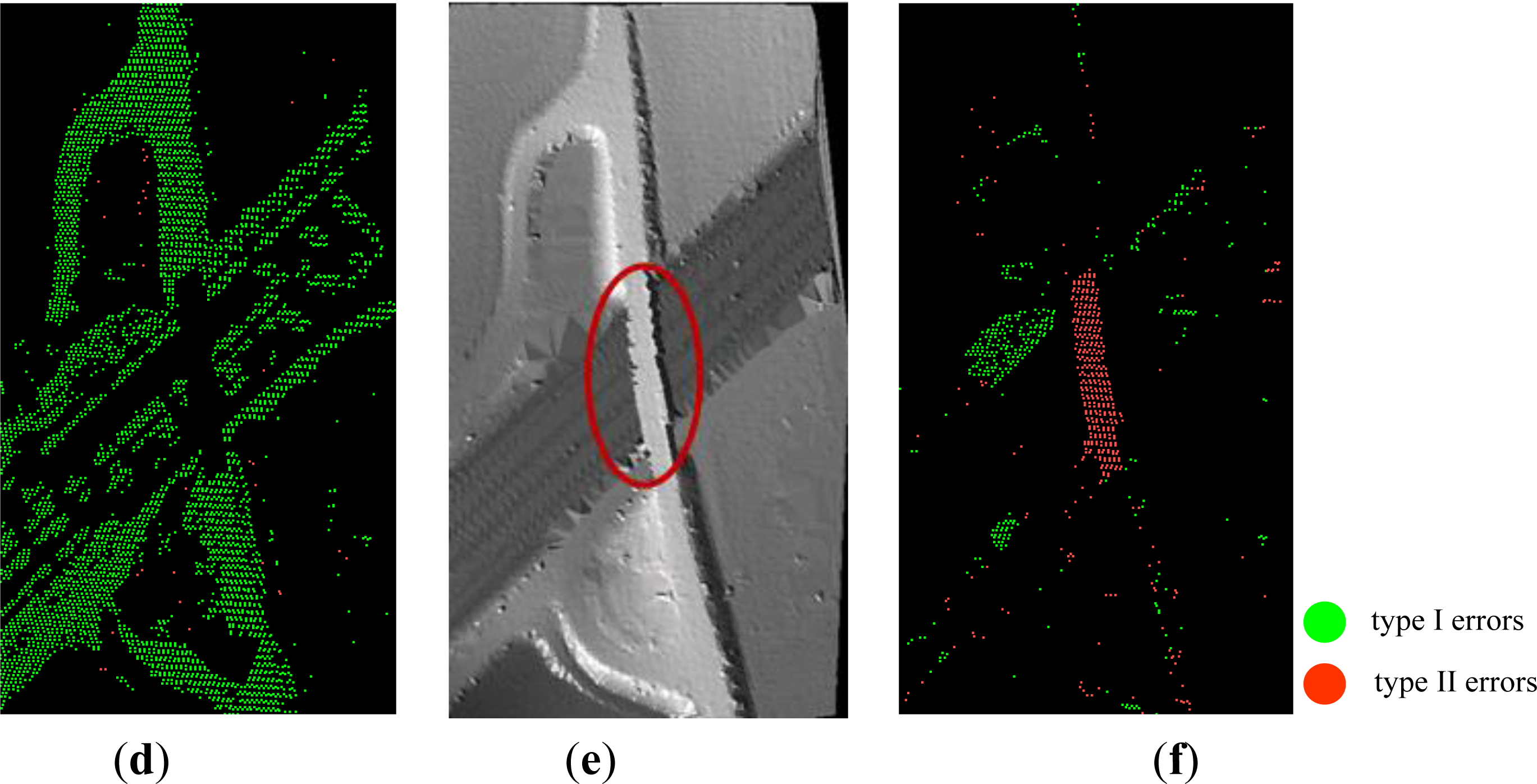
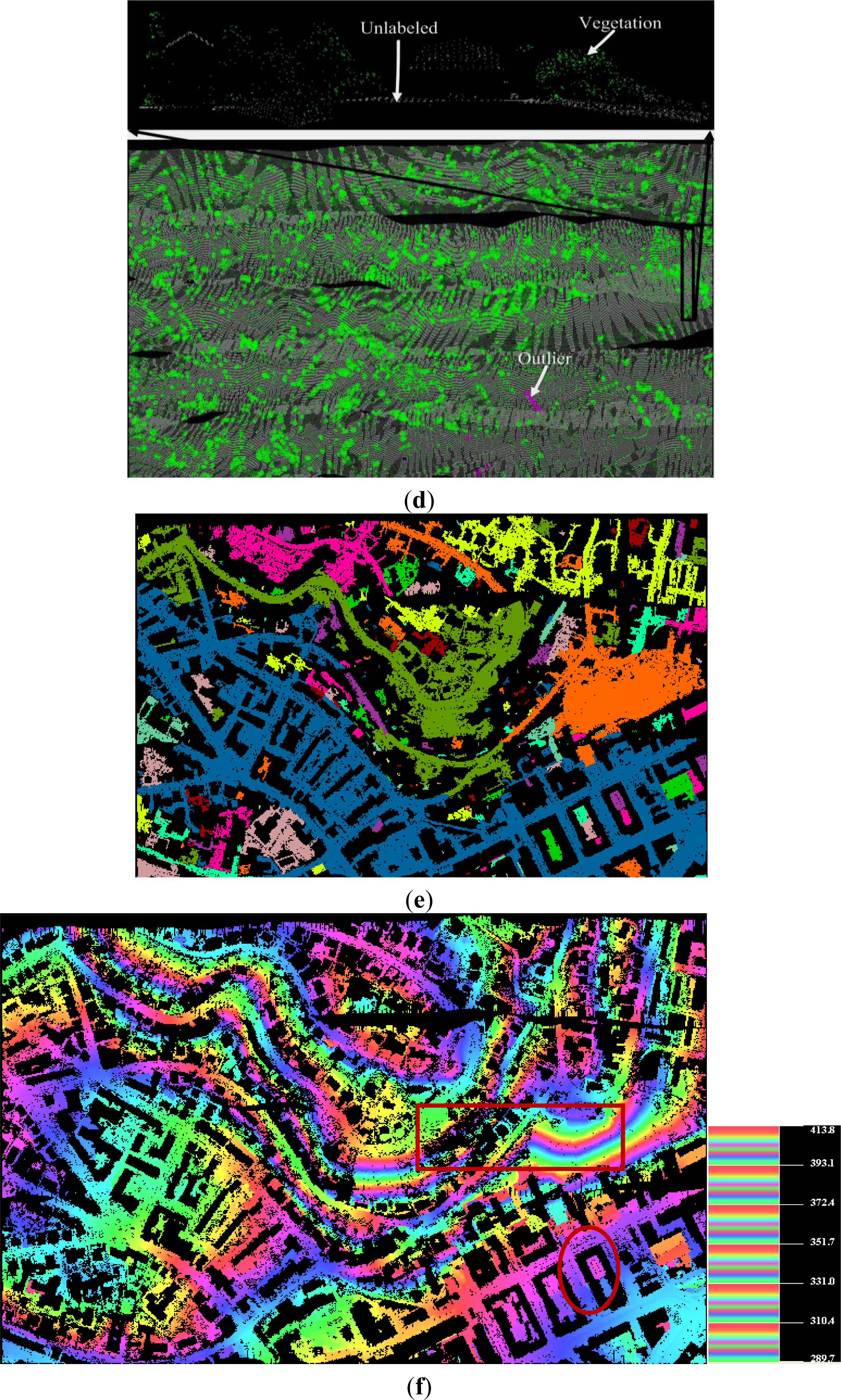
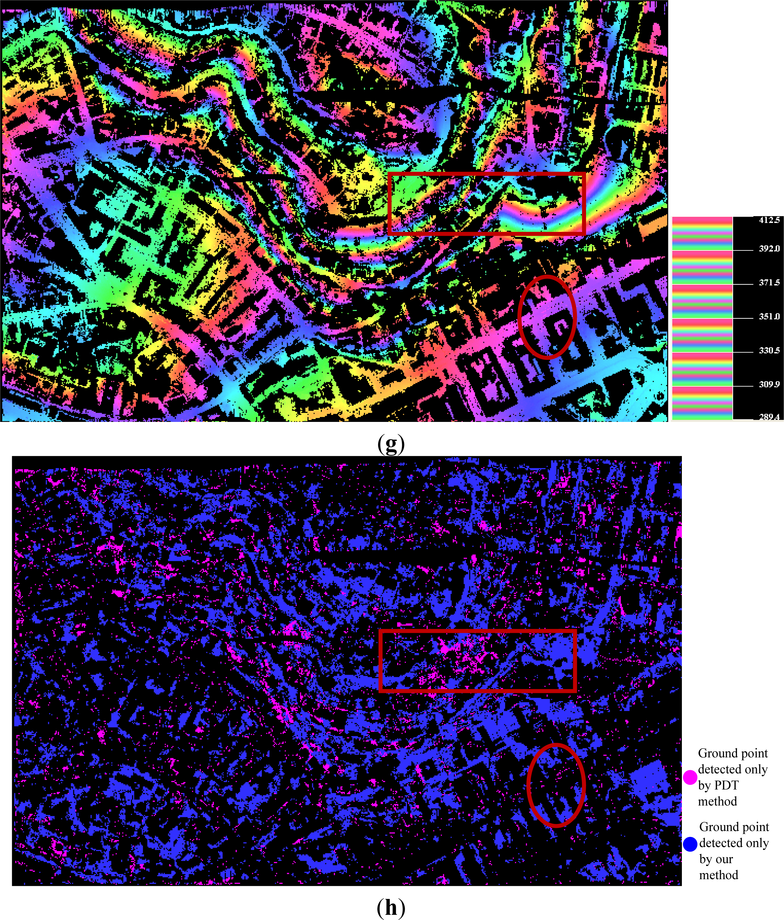
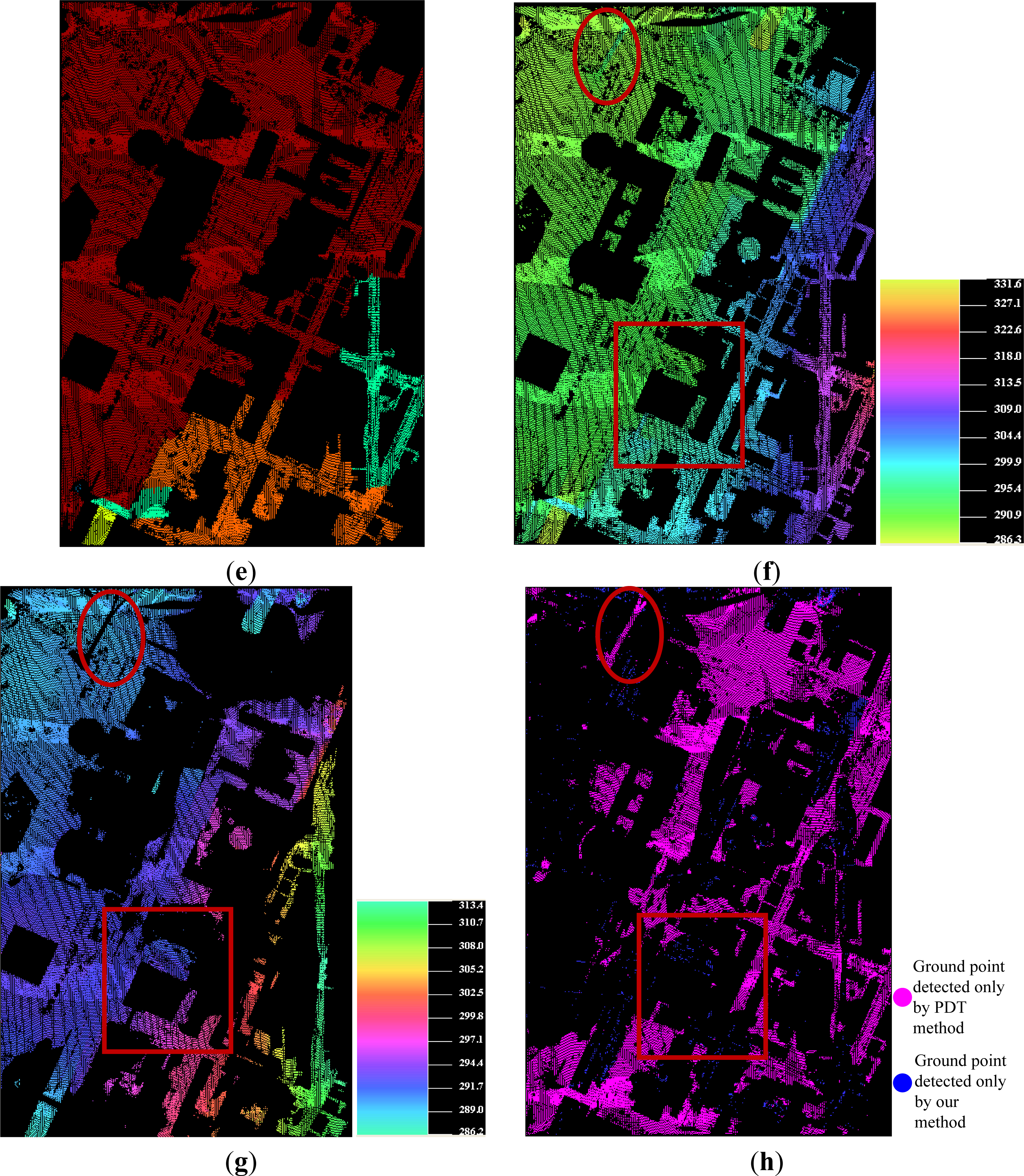
• if the objects are closely attached to the underlying terrain surface, as the bridge shown in the ellipse regions of Figures 6f and 11e;
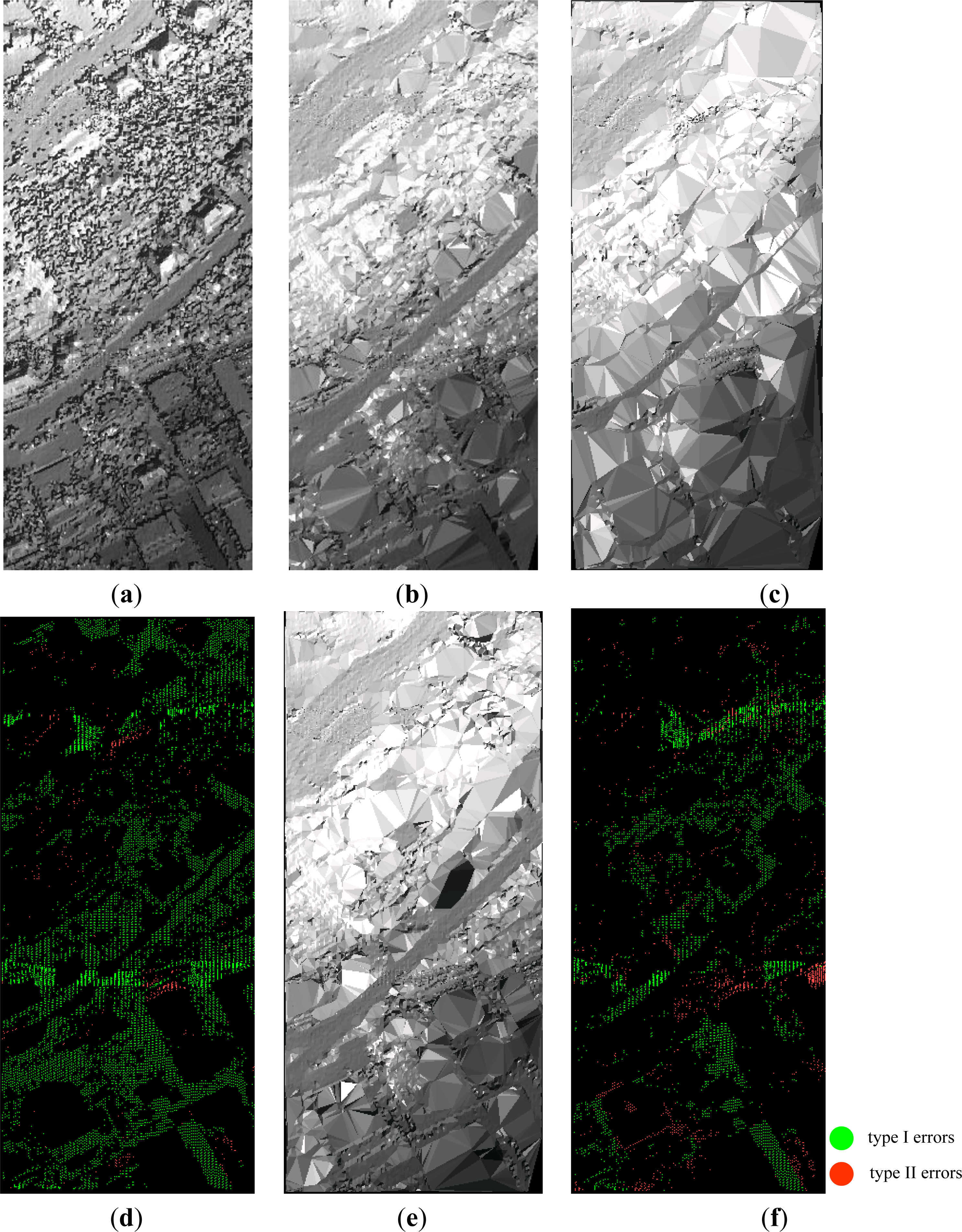
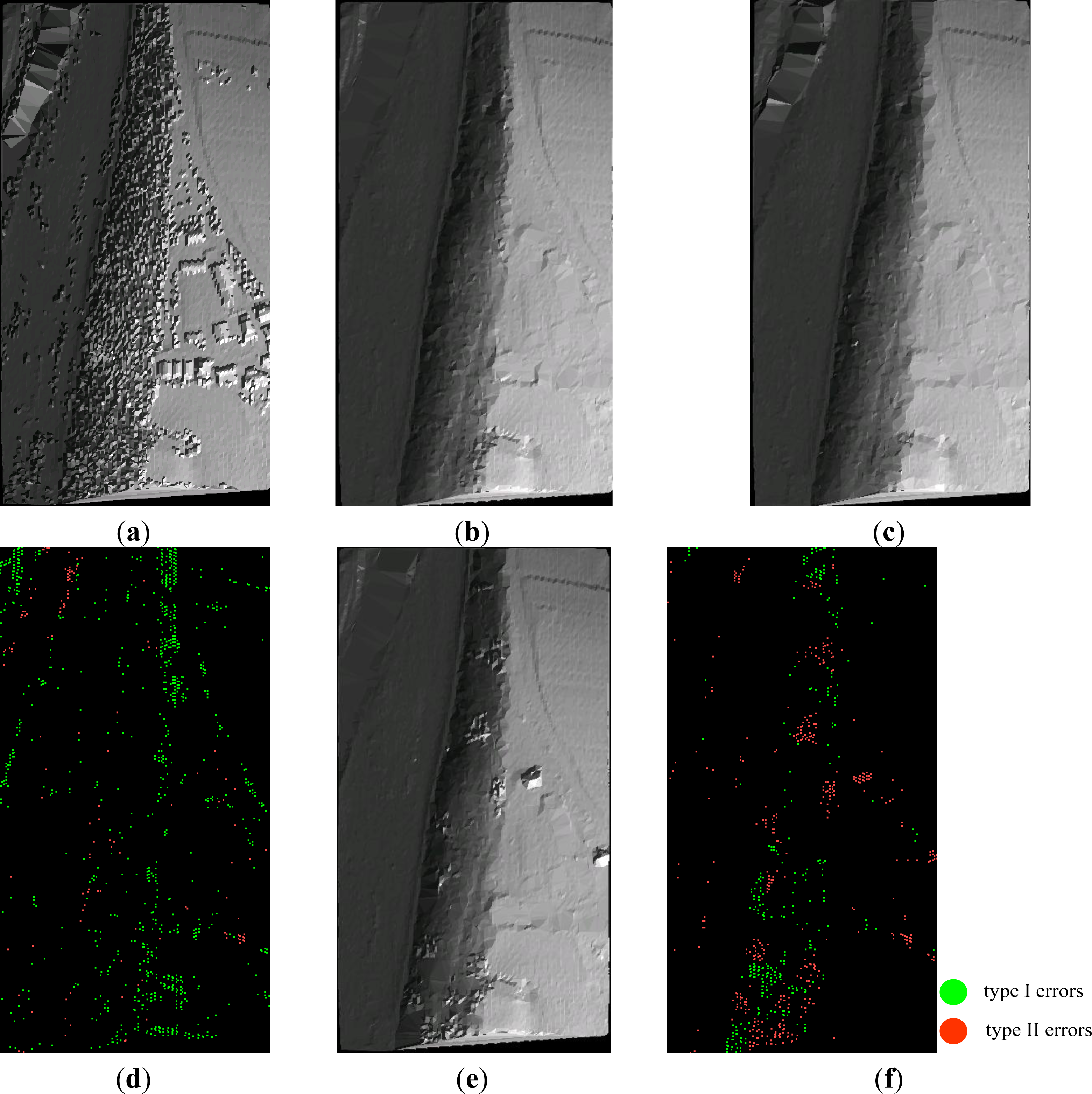
• if the objects are both small and very close to the ground surfaces, as shown in Figure 9f.

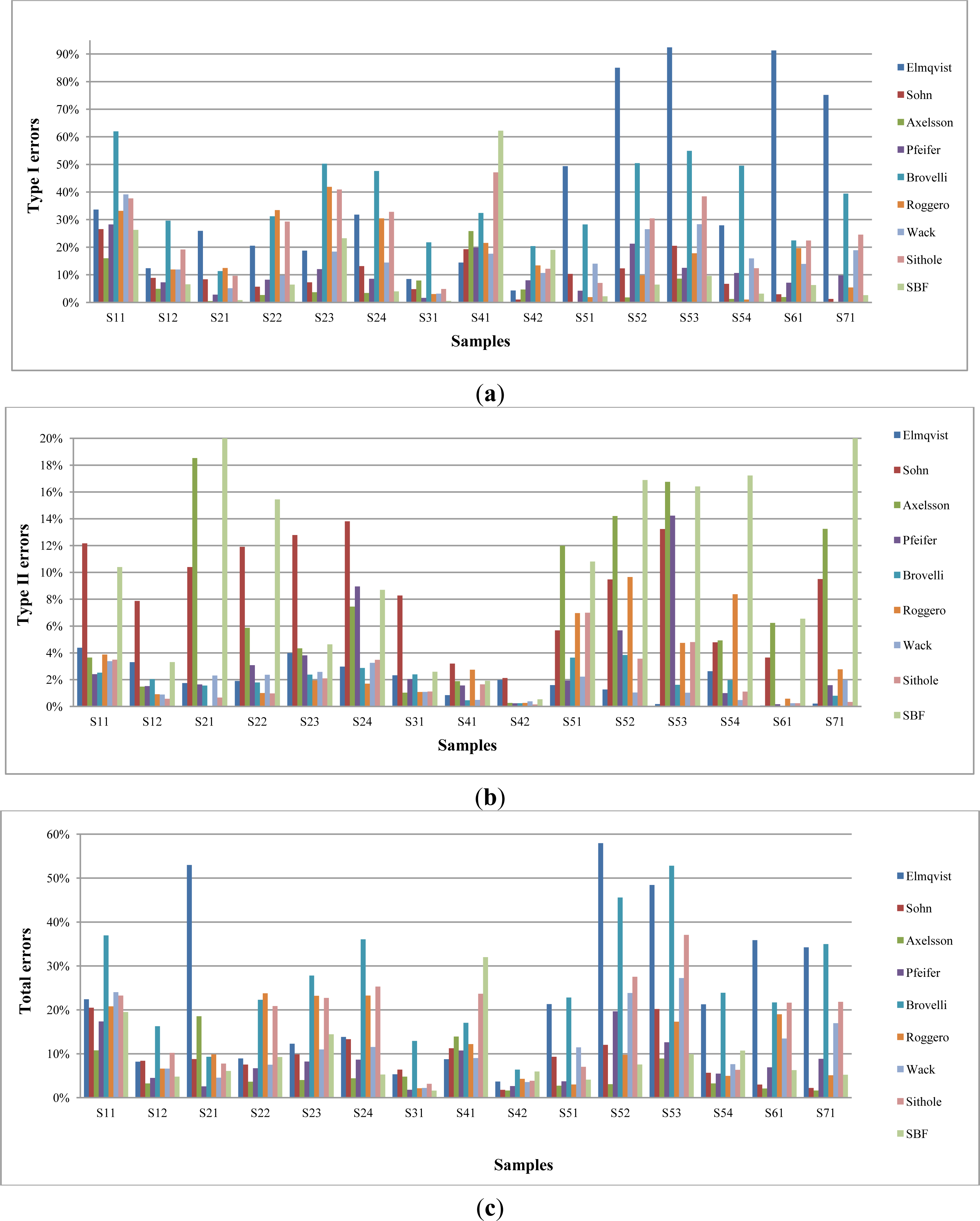
4.4. Performance Evaluation between SBF and PTD

Both qualitative and quantitative assessments are made to evaluate the performances of the two filters. Particularly, qualitative assessments are made by visually comparing the seven filtered results and the 15 references. Visual assessment shows that, both the classic PTD method and the SBF method are robust to various types of complex landscapes such as large buildings, irregularly shaped buildings, mixture of vegetation and buildings on flat terrains; and they are both sensitive to the data gaps, because the data gaps may cause the terrain not continuous. However, the PTD algorithm fails to remove the points belonging to the lower parts of the objects, and fails to preserve the ground measurements in the cases of steep slopes, mixture of vegetation and buildings on a hillside, and just buildings on a hillside. Fortunately, the SBF method is more likely to make a correct judgment when the PTD algorithm fails. On the other side, compared with the PTD algorithm, the SBF method fails to identify the object measurements which are connected to the terrain surface through a smooth transition such as the very low buildings, as shown in the ellipse region in Figure 5e–g, and the bridges, as shown in the ellipse region in Figure 6e–g.

Additionally, the quantitative assessments are followed the one proposed in ISPRS filter test [17]. Three kinds of errors are calculated, namely, type I errors (i.e., omission errors), type II errors (i.e., commission errors), and total errors. The type I error is the percentage of bare earth returns misclassified as object returns, whereas the type II error is the percentage of object returns misclassified as bare earth returns, and the total error is the percentage of any misclassified points. The three types of errors of the two filters in the 15 references are listed in

Table 3. Three types of errors of the two filters, i.e., PTD method and SBF method.

Dataset NO.	Type of Error	PTD (%)	SBF (%)	Dataset NO./Types	Type of Error	PTD (%)	SBF (%)
Sample 11	I	51.29	26.28	Sample 51	I	6.05	2.22
	II	3.40	10.40		II	3.59	10.81
	T	30.85	19.50		T	5.51	4.09
Sample 12	I	21.13	6.56	Sample 52	I	21.11	6.46
	II	1.84	3.31		II	3.77	16.89
	T	11.72	4.78		T	19.29	7.56
Sample 21	I	1.67	0.85	Sample 53	I	28.98	9.62
	II	8.97	24.45		II	1.66	16.41
	T	3.29	6.08		T	27.87	9.90
Samp22	I	44.74	6.43	Sample 54	I	9.09	3.16
	II	3.08	15.44		II	2.27	17.23
	T	31.74	9.24		T	5.43	10.72
Sample 23	I	53.77	23.21	Sample 61	I	27.18	6.26
	II	3.22	4.64		II	4.15	6.55
	T	29.85	14.43		T	26.39	6.27
Sample 24	I	58.81	3.99	Sample 71	I	32.19	2.62
	II	10.98	8.70		II	1.86	25.65
	T	45.68	5.28		T	28.76	5.22
Sample 31	I	7.87	0.54	Minimum	I	1.67	0.54
	II	4.13	2.59		II	0.82	0.54
	T	6.15	1.61		T	3.29	1.61
Sample 41	I	70.31	62.22	Maximum	I	70.31	62.22
	II	0.82	1.92		II	10.98	25.65
	T	35.48	32.00		T	35.48	32.00
Sample 42	I	19.37	19.02	Average	I	30.24	11.96
	II	1.40	0.54		II	3.68	11.06
	T	6.66	5.95		T	20.98	9.51

.

The statistics in Table 3 suggest that, both filters could achieve high accuracies on the seven datasets, and the total error is less than 35.48% for all the filtered results, as shown in Table 3 and Figure 13c. On the contrast, they both acquire low accuracies in the area with data gaps such as Sample 41. For Sample 41, they both have the highest type I errors and total errors among all the references, as listed in Table 3. However, generally, the SBF method has significantly lower type I error and total error than the PTD method. Specifically, among the 15 references, there are 15 cases where the type I errors of the SBF method are lower than the PTD method, and there are 13 cases except the Sample 21 and Sample 54 where the total error of the SBF method are lower than the PTD approach, as shown in Figure 13a,c. On average, compared with the PTD algorithm, the type I error and total error of the SBF method are approximately reduced by 18.26% and 11.47%, respectively. However, the classic PTD approach also has its advantage in avoiding type II errors. The statistics in Table 3 tell us that, there are 12 cases where the SBF method has higher type II errors than the PTD algorithm, as shown in Figure 13b. However, the above disadvantage of the SBF method is not fatal. Considering that the SBF method is likely to have lower type I errors and total errors, SBF will need less human involvements compared with the PTD method, because the cost of repairing the type II errors is far lower than the ones of repairing the type I error in the stage of manual operation after automatic filtering [17].

Another disadvantage of the SBF approach is that it needs four more specified parameters needed for the segmentation, as illustrated in Section 3.2. Based on the scene complexity and statistics in Table 3, CSite2 and Sample 23 are selected to analyze the sensitivity of the four parameters and the effect on three types of errors, because the Sample 23 has higher complexity and both of the classic PTD method and the SBF method don’t perform well in this sample; and the results are shown in Figure 14. For k ∈ [10, 30] and the other parameters are fixed, the type I errors decrease from 28.91% to 18.01%, the type II errors increase from 3.87% to 4.89%, and the total errors decrease from 17.07% to 11.81%. The above obvious difference owns to the sensitivity of k to the plane fitting in PCSS if k is not large enough. However, when k is approaching to 20, the three types will not change significantly. Actually, for k ∈ [18, 26], the type I errors decrease from 22.21% to 22.00%, the type II errors decrease from 4.66% to 4.48%, the total errors decrease from 13.91% to 13.81%, despite there is also a slight fluctuation when k = 22 for the type I error and the type II error. Similar trends happen to the other three parameters. Particularly, for α ∈ [4°, 11°] or r ∈ [0.2 m, 0.4 m] or d' ∈ [2.5 m, 4.0 m], and the other parameters are fixed, the three types of errors will not change significantly, as shown in Figure 14b–d respectively. In a word, the three types are not sensitive to the change of values of the four parameters within some ranges. Thus, we can get similar results if we chose slightly different values. The Figure 14 also suggests that we have not fine-tuned these particular examples so the results come out favorably, but just made decisions on experiences, because k = 20, r = 0.3 m, d' = 3 m and α = 5° is not the optimal values in view of three types of errors. On the other hand, the statistics in Figure 14c suggest that the over-segmentation or under-segmentation induced by the bad segmentation parameters will lead to bad filtering result. For example, in Figure 14c, when k = 20, r = 0.3 m, d' = 1.0 m and α = 5°, the three types of errors are approaching the ones of the classic PDT filter. Furthermore, from the parameters in Table 1, we conclude that k = 20, r = 0.3 m, d' = 3.0 m and α = 5° or 10° or 15° turned out to be feasible for the seven datasets. In other words, the additional four parameters do not significantly add complexity to the SBF method if the time cost was not considered. From the above statistics and analysis, we conclude that the SBF method has a significant reduction of the type I errors and total errors compared to the PTD method without significantly adding to the complexity of the algorithm. However, the optimal values of the four parameters may need adaptation for the other point cloud datasets in practice.

A further disadvantage of the SBF method is that it needs more computation time compared to the PTD method, because of the segmentation and the iterative judgment of segments, as illustrated in Section 2. The time costs are recorded and listed in Table 2. On average, time cost of the SBF method is 18.3 times more than the PDT method on the same computer. However, this paper focuses on a filter’s accuracy rather than efficiency, and the efficiency of a filter method may be solved if the algorithm was optimized or parallel computing was considered.

The advantages of the SBF method result from the following three factors. The first one is the adopting of the point cloud segmentation in the process of filtering. Particularly, the PCSS method will expand the set of initial ground points to a large extent if the natural terrain is smooth enough, as shown in both of Figures 5d and 6d. The statistics in Table 2 suggest the proportion of selected ground seed points by PCSS to the finial detected ground points is approaching approximately 77%. As a result, the increased number of ground seed points reduces the possibility of omitting the remaining ground measurements for the SBF algorithm. The second one is the adopting of multiple echoes analysis. The multiple echoes analysis is helpful to detect the vegetation measurements, which will reduce the number of points to be judged and also reduce the possible errors. The last but not least factor is the inheritance of the flow chart of classic PTD method. As mentioned above, the PTD method is an excellent filter, and it has been widely applied due to the popularization of the TerraSolid commercial software. The SBF approach makes best use of the flow chart of the classic PTD algorithm. However, embedding the PCSS into the PTD is also a double-edged sword. The point cloud segmentation also makes the SBF method more likely regard some small object points attached to the terrain as ground points, which probably increases the type II errors for the SBF method if the small objects were abundant in this scene, as shown in Table 3 and Figure 13b.

4.5. Performance Evaluation between SBF and the Others

As mentioned above, there are eight filtering algorithms presented by Sithole and Vosselman [17]. There is comparability between them on the filtering accuracy. Thus, the quantitative assessments are also performed between the SBF method and the eight filters. The three types of errors of the classic eight filters and the SBF method in the 15 references are displayed in Figure 15a–c, respectively.

Figure 15a,b suggest that, the SBF method has low type I errors and total errors. Specifically, among the 15 references, there are two cases where the type I errors of the SBF method are the lowest, there are five cases where the type I errors of the SBF method are the second lowest, and there are four cases where the type I errors of the SBF method are the third lowest. Similarly, there is one case where the total errors of the SBF method are the lowest, there are four cases where the total errors of the SBF method are the second lowest, and there are also four cases where the total errors of the SBF method are the third lowest. Moreover, both of the type I error and total error of the SBF method is lower than the corresponding average of the eight filters. However, most of the eight filtering approaches have lower type II errors than the SBF method, as shown in Figure 15b. Totally, the SBF method has lower type I error and total error but higher type II error than most of the classic eight filtering methods, which suggests the same advantages and disadvantages of the SBF method as in Section 4.4.

5. Conclusions

Filtering is one of the core post-processing steps for ALS point clouds, and many filters have been proposed to solve this problem. Among them, PTD is widely applied as one of the surface-based ones. However, the PTD fails to remove the lower parts of the objects and preserve the ground measurements in steep terrain areas even if the mirroring technique is adopted. Practices suggest that the combination of surface-based filters and the segmentation-based filters is capable of overcoming the above shortcomings. Thus, a segmentation-based filtering method is proposed therein by integrating the PTD framework and PCSS method. The experiments make use of the 7 datasets of ISPRS Commission III/Working Group III to verify the SBF method; moreover, the 15 reference samples from the sub-areas are used to calculate the accuracies of the proposed approach. The results suggest that both the SBF method and the classic PTD are robust to various types of landscapes. However, the SBF approach is better than the classic PTD method in removing the vehicle measurements and preserving the ground measurements. Particularly, it may have significant lower type I errors and total errors than the PTD algorithm despite that it may have higher type II errors, which will reduce the cost of the following manual correction. However, the SBF method may fail when it is faced with objects, which are attached to the ground, such as bridges, ramps, etc.; and it is also sensitive to the large data gaps. Similar conclusions could be made if the SBF method is compared with the eight filtering algorithms presented by Sithole and Vosselman [17]. The future work will focus on the improvement of the proposed filter to reduce the type II errors, markov random field model [48] is introduced to analyze the spatial topology of the segments, multi-source data fusion [49] is employed and parallel computing is performed to promote the efficiency.

References

1. Zhang, J.X.; Lin, X.G.; Ning, X.G. SVM-based classification of segmented airborne LiDAR point clouds in urban areas. Remote Sens 2013, 5, 3749–3775. [Google Scholar]
2. Shan, J.; Sampath, A. Urban DEM generation from raw Lidar data: A labeling algorithm and its performance. Photogramm. Eng. Remote Sens 2005, 71, 217–226. [Google Scholar]
3. Zhang, J.X.; Lin, X.G. Filtering airborne LiDAR data by embedding smoothness-constrained segmentation in progressive TIN densification. ISPRS J. Photogramm 2013, 81, 44–59. [Google Scholar]
4. Maas, H.G.; Vosselman, G. Two algorithms for extracting building models from raw laser altimetry data. ISPRS J. Photogramm. Remote Sens 1999, 54, 153–163. [Google Scholar]
5. Rutzinger, M.; Rottensteiner, F.; Pfeifer, N. A comparison of evaluation techniques for building extraction from airborne laser scanning. IEEE J. Sel. Top. Appl. Earth Obs. Remote Sens 2009, 2, 11–20. [Google Scholar]
6. Huang, H.; Brenner, C.; Sester, M. A generative statistical approach to automatic 3D building roof reconstruction from laser scanning data. ISPRS J. Photogramm. Remote Sens 2013, 79, 29–43. [Google Scholar]
7. Wang, R. 3D building modeling using images and LiDAR: A review. Int. J. Image Data Fusion 2013, 4, 273–292. [Google Scholar]
8. Oude Elberink, S.; Vosselman, G. 3D information extraction from laser point clouds covering complex road junctions. Photogramm. Rec 2009, 24, 23–36. [Google Scholar]
9. Koch, B.; Heyder, U.; Weinacker, H. Detection of individual tree crowns in airborne LiDAR data. Photogramm. Eng. Remote Sens 2006, 72, 357–363. [Google Scholar]
10. Liu, J.P.; Shen, J.; Zhao, R.; Xu, S.H. Extraction of individual tree crowns from airborne LiDAR data in human settlements. Math. Comput. Model 2013, 58, 524–535. [Google Scholar]
11. Hyyppä, J.; Yu, X.; Hyyppä, H.; Vastaranta, M.; Holopainen, M.; Kukko, A.; Kaartinen, H.; Jaakkola, A.; Vaaja, M.; Koskinen, J.; et al. Advances in forest inventory using airborne laser scanning. Remote Sens 2012, 4, 1190–1207. [Google Scholar]
12. Wang, C.; Menenti, M.; Stoll, M.P.; Feola, A.; Belluco, E.; Marani, M. Separation of ground and low vegetation signatures in LiDAR measurements of salt-marsh environments. IEEE Trans. Geosci. Remote Sens 2009, 47, 2014–2023. [Google Scholar]
13. French, J.R. Airborne LiDAR in support of geomorphological and hydraulic modelling. Earth Surf. Process. Landf 2003, 28, 321–335. [Google Scholar]
14. Hutton, C.J.; Brazier, R.E. Quantifying riparian zone structure from airborne LiDAR: Vegetation filtering, anisotropic interpolation, and uncertainty propagation. J. Hydrol 2012, 442–443, 36–45. [Google Scholar]
15. Lin, X.G.; Zhang, R.; Shen, J. A template-matching based approach for extraction of roads from very high resolution remotely sensed imagery. Int. J. Image Data Fusion 2012, 3, 149–168. [Google Scholar]
16. Meng, X.; Currit, N.; Zhao, K. Ground filtering algorithms for airborne LiDAR data: A review of critical issues. Remote Sens 2010, 2, 833–860. [Google Scholar]
17. Sithole, G.; Vosselman, G. Experimental comparison of filter algorithms for bare earth extraction from airborne laser scanning point clouds. ISPRS J. Photogramm. Remote Sens 2004, 59, 85–101. [Google Scholar]
18. Tóvári, D.; Pfeifer, N. Segmentation based robust interpolation-a new approach to laser data filtering. Int. Arch. Photogramm. Remote Sens 2005, 36, 79–84. [Google Scholar]
19. Kraus, K.; Pfeifer, N. Determination of terrain models in wooded areas with airborne laser scanner data. ISPRS J. Photogramm. Remote Sens 1998, 53, 193–203. [Google Scholar]
20. Vosselman, G. Slope based filtering of laser altimetry data. Int. Arch. Photogramm. Remote Sens 2000, 33, 935–942. [Google Scholar]
21. Sithole, G.; Vosselman, G. Filtering of laser altimetry data using a slope adaptive filter. Int. Arch. Photogramm. Remote Sens 2001, 34, 203–210. [Google Scholar]
22. Susaki, J. Adaptive slope filtering of airborne LiDAR data in urban areas for digital terrain model (DTM) generation. Remote Sens 2012, 4, 1804–1819. [Google Scholar]
23. Chen, Q.; Gong, P.; Baldocchi, D.; Xie, G. Filtering airborne laser scanning data with morphological methods. Photogramm. Eng. Remote Sens 2007, 73, 175–185. [Google Scholar]
24. Zhang, K.Q.; Chen, S.C.; Whitman, D.; Shyu, M.L.; Yan, J.H.; Zhang, C.C. A progressive morphological filter for removing nonground measurements from airborne LIDAR data. IEEE Trans. Geosci. Remote Sens 2003, 41, 872–882. [Google Scholar]
25. Briese, C.; Pfeifer, N.; Dorninger, P. Applications of the robust interpolation for DTM determination. Int. Arch. Photogramm. Remote Sens 2002, 34, 55–61. [Google Scholar]
26. Kobler, A.; Pfeifer, N.; Ogrinc, P.; Todorovski, L.; Oštir, K.; Džeroski, S. Repetitive interpolation: A robust algorithm for DTM generation from aerial laser scanner data in forested terrain. Remote Sens. Environ 2007, 108, 9–23. [Google Scholar]
27. Axelsson, P.E. DEM generation from laser scanner data using adaptive TIN models. Int. Arch. Photogramm. Remote Sens 2000, 32, 110–117. [Google Scholar]
28. Zhu, X.K.; Toutin, T. Land cover classification using airborne LiDAR products in Beauport, Québec, Canada. Int. J. Image Data Fusion 2013, 4, 252–271. [Google Scholar]
29. Lohmann, P. Segmentation and filtering of laser scanner digital surface models. Int. Arch. Photogramm. Remote Sens 2002, 34, 311–315. [Google Scholar]
30. Lee, I. A Feature Based Approach to Automatic Extraction of Ground Points for DTM Generation from LiDAR Data. Proceedings of the ASPRS Annual Conference, Denver, CO, USA, 23–28 May 2004.
31. Sithole, G.; Vosselman, G. Filtering of airborne laser scanner data based on segmented point clouds. Int. Arch. Photogramm. Remote Sens 2005, 36, 66–71. [Google Scholar]
32. Shen, J.; Liu, J.P.; Lin, X.G.; Zhao, R. Object-based classification of airborne light detection and ranging point clouds in human settlements. Sens. Lett 2012, 10, 221–229. [Google Scholar]
33. Yan, M.; Blaschke, T.; Liu, Y.; Wu, L. An object-based analysis filtering algorithm for airborne laser scanning. Int. J. Remote Sens 2012, 33, 7099–7116. [Google Scholar]
34. Arya, S.; Mount, D.M.; Netanyahu, N.S.; Silverman, R.; Wu, A.Y. An optimal algorithm for approximate nearest neighbor searching in fixed dimensions. J. ACM 1998, 45, 891–923. [Google Scholar]
35. Filin, S.; Pfeifer, N. Segmentation of airborne laser scanning data using a slope adaptive neighborhood. ISPRS J. Photogramm. Remote Sens 2006, 60, 71–80. [Google Scholar]
36. Melzer, T. Non-parametric segmentation of ALS point clouds using mean shift. J. Appl. Geod 2007, 1, 159–170. [Google Scholar]
37. Wang, M.; Tseng, Y.H. Automatic segmentation of LiDAR data into coplanar point clusters using an octree-based split-and-merge algorithm. Photogramm. Eng. Remote Sens 2010, 76, 407–420. [Google Scholar]
38. Rottensteiner, F. Automatic generation of high-quality building models from LiDAR data. IEEE Comput. Graph. Appl 2003, 23, 42–50. [Google Scholar]
39. Vosselman, G.; Klein, R. Visualization and Structuring of Point Clouds. In Airborne and Terrestrial Laser Scanning, 1st ed; Vosselman, G., Maas, H.G., Eds.; Whittles Publising: Dunbeath, UK, 2010; pp. 43–79. [Google Scholar]
40. Chen, D.; Zhang, L.; Li, J.; Liu, R. Urban building roof segmentation from airborne lidar point clouds. Int. J. Remote Sens 2012, 33, 6497–6515. [Google Scholar]
41. Rabbani, T. Automatic Reconstruction of Industrial Installations Using Point Clouds and Images. Netherlands Commission of Geodesy, Delft, The Netherlands, 2006. [Google Scholar]
42. Moffiet, T.; Mengersen, K.; Witte, C.; King, R.; Denham, R. Airborne laser scanning: Exploratory data analysis indicates potential variables for classification of individual trees or forest stands according to species. ISPRS J. Photogramm. Remote Sens 2005, 59, 289–309. [Google Scholar]
43. Wang, O. Using Aerial LiDAR to Segment and Model Buildings. University of California, Santa Cruz, CA, USA, 2006. [Google Scholar]
44. Darmawati, A.T. Utilization of Multiple Echo Information for Classification of Airborne Laser Scanning Data. International Institute for Geo-information Science and Observation, Enschede, The Netherlands, 2008. [Google Scholar]
45. Höfle, B.; Hollaus, M.; Hagenauer, J. Urban vegetation detection using radiometrically calibrated small-footprint full-waveform airborne LiDAR data. ISPRS J. Photogramm. Remote Sens 2012, 67, 134–147. [Google Scholar]
46. A Two-Dimensional Quality Mesh Generator and Delaunay Triangulator. Available online: http://www.cs.cmu.edu/~quake/triangle.html (accessed on 11 October 2011).
47. ANN: A Library for Approximate Nearest Neighbor Searching. Available online: http://www.cs.umd.edu/~mount/ANN/ (accessed on 15 March 2010).
48. Seetharaman, K.; Palanivel, N. Texture characterization, representation, description, and classification based on full range gaussian markov random field model with bayesian approach. Int. J. Image Data Fusion 2013, 4, 342–362. [Google Scholar]
49. Akiwowo, A.; Eftekhari, M. Feature-based detection using Bayesian data fusion. Int. J. Image Data Fusion 2013, 4, 308–323. [Google Scholar]
Figure 1. Typical errors of Axelsson’s progressive TIN (triangular irregular network) densification (PTD) filter. (a) A point cloud around a step edge; (b) Filtering result of the point cloud in (a); (c) A point cloud in urban area with dense vehicles; (d) Filtering result of the point cloud in (c).
Remotesensing 06 01294f1
Figure 2. Flow chart of the segmentation-based filtering (SBF) method.
Remotesensing 06 01294f2
Figure 3. Parameters of the point cloud smooth segmentation (PCSS) segmentation. For a seed point with normal vector and a fitted plane across the seed point, select its neighboring points whose 3D distance to the seed point within d'. Among the neighboring points, add the points, whose angle difference to seed points is less than α and whose distance to the fitted plane is less than r, to the segment.
Remotesensing 06 01294f3
Figure 4. The progress of SBF method and some needed parameters. (a) A point cloud; (b) Result of point cloud segmentation; (c) Selection of ground seed segments; (d) Construction of TIN by the points in (c); (e) Measurement of angle and distance; (f) Mirroring process.
Remotesensing 06 01294f4
Figure 5. Filtering and results of testing data about CSite1: (a) The remaining point cloud after outlier removal; (b) TIN of the data in (a); (c) Segmentation result of PCSS; (d) Detected vegetation measurements by multiple echoes analysis of segments; (e) Detected ground seed segments colored by the labeling number; (f) Detected ground measurements by SBF method; (g) Detected ground measurements by the classic PTD method; (h) Differences between (f) and (g).
Remotesensing 06 01294f5aRemotesensing 06 01294f5bRemotesensing 06 01294f5c
Figure 6. Filtering and results of testing data about CSite2: (a) The remaining point cloud after outlier removal; (b) TIN of the data in (a); (c) Segmentation result of PCSS; (d) Detected vegetation measurements by multiple echoes analysis of segments; (e) Detected ground seed segments colored by the labeling number; (f) Detected ground measurements by SBF method; (g) Detected ground measurements by the classic PTD method; (h) Differences between (f) and (g).
Remotesensing 06 01294f6aRemotesensing 06 01294f6b
Figure 7. Filtering and results of reference data of Sample 11: (a) The digital surface model (DSM); (b) The reference DEM; (c) The DEM generated from the result of the PTD method; (d) The type I errors, type II errors of the PTD method; (e) The DEM generated from the result of the SBF method; (f) The type I errors, type II errors of the SBF method. Note that both of the DSM and the DEM are TIN-based.
Remotesensing 06 01294f7
Figure 8. Filtering and results of reference data of Sample 24: (a) The DSM; (b) The reference DEM; (c) The DEM generated from the result of the PTD method; (d) The type I errors, type II errors of the PTD method; (e) The DEM generated from the result of the SBF method; (f) The type I errors, type II errors of the SBF method. Note that both of the DSM and the DEM are TIN-based.
Remotesensing 06 01294f8
Figure 9. Filtering and results of reference data of Sample 51: (a) The DSM; (b) The reference DEM; (c) The DEM generated from the result of the PTD method; (d) The type I errors, type II errors of the PTD method; (e) The DEM generated from the result of the SBF method; (f) The type I errors, type II errors of the SBF method. Note that both of the DSM and the DEM are TIN-based.
Remotesensing 06 01294f9
Figure 10. Filtering and results of reference data of Sample 53: (a) The DSM; (b) The reference DEM; (c) The DEM generated from the result of the PTD method; (d) The type I errors, type II errors of the PTD method; (e) The DEM generated from the result of the SBF method; (f) The type I errors, type II errors of the SBF method. Note that both of the DSM and the DEM are TIN-based.
Remotesensing 06 01294f10
Figure 11. Filtering and results of reference data of Sample 71: (a) The DSM; (b) The reference DEM; (c) The DEM generated from the result of the PTD method; (d) The type I errors, type II errors of the PTD method; (e) The DEM generated from the result of the SBF method; (f) The type I errors, type II errors of the SBF method. Note that both of the DSM and the DEM are TIN-based.
Remotesensing 06 01294f11aRemotesensing 06 01294f11b
Figure 12. Filtering and results of reference data of Sample 12: (a) The DEM generated from the result of the PTD method; (b) The DEM generated from the result of the SBF method. Note that the two DEM are TIN-based.
Remotesensing 06 01294f12
Figure 13. Comparison of the three types of errors for the two methods: (a) Type I errors of different algorithms for the samples; (b) Type II errors of different algorithms for the samples; (c) Total errors of the two algorithms for the samples. Note “S” is abbreviation of “Sample” for the horizontal captions.
Remotesensing 06 01294f13
Figure 14. Analysis on sensitivity of the input parameters k and α respectively, and its effect on the three types of errors for the Sample 23. (a) Values of k and the corresponding three types of errors when r = 0.3 m, d' = 3.0 m and α = 5°; (b) Values of α and the corresponding three types of errors when k = 20, r = 0.3 m, d' = 3.0 m; (c) Values of d' and the corresponding three types of errors when k = 20, r = 0.3 m, α = 5°; (d) Values of r and the corresponding three types of errors when k = 20, d' = 3.0 m, α = 5°.
Remotesensing 06 01294f14
Figure 15. Comparison of the three types of errors for the SBF method and the eight methods in [17]: (a) Type I errors of different algorithms for the samples; (b) Type II errors of different algorithms for the samples; (c) Total errors of the two algorithms for the samples. Note “S” is abbreviation of “Sample” for the horizontal captions.
Remotesensing 06 01294f15