Article

Monitoring Wetlands Ecosystems Using ALOS PALSAR (L-Band, HV) Supplemented by Optical Data: A Case Study of Biebrza Wetlands in Northeast Poland

Institute of Geodesy and Cartography, Department of Remote Sensing, Modzelewskiego 27, Warsaw 02-679, Poland
*
Author to whom correspondence should be addressed.
Remote Sens. 2014, 6(2), 1605-1633; https://doi.org/10.3390/rs6021605
Submission received: 7 January 2014 / Revised: 21 January 2014 / Accepted: 12 February 2014 / Published: 20 February 2014
(This article belongs to the Special Issue Remote Sensing of Peatlands I)

Abstract

:
The aim of the study was to elaborate the remote sensing methods for monitoring wetlands ecosystems. The investigation was carried out during the years 2002–2010 in the Biebrza Wetlands. The meteorological conditions at the test site varied from extremely dry to very wet. The authors propose applying satellite remote sensing data acquired in the optical and microwave spectrums to classify wetlands vegetation habitats for the assessment of vegetation changes and estimation of wetlands’ biophysical properties to improve monitoring of these unique, very often physically impenetrable, areas. The backscattering coefficients (σ°) calculated from ALOS PALSAR FBD (Advanced Land Observing Satellite, Phased Array type L-band Synthetic Aperture Radar, Fine Beam Dual Mode) images registered at cross polarization HV on 12 May 2008 were used to classify the main wetland communities using ground truth observations and the visual interpretation method. As a result, the σ° values were distributed among the six wetlands’ vegetation classes: scrubs, sedges-scrubs, sedges, reeds, sedges-reeds, rushes, and the areas of each community and changes were assessed. Also, the change in the biophysical variable as Leaf Area Index (LAI) is described using the information from PALSAR data. Strong linear relationships have been found between LAI and σ° derived for particular wetland classes, which then were applied to elaborate the maps of LAI distribution. The other variables used to characterize the changing environmental conditions are: surface temperature (Ts) calculated from NOAA AVHRR (National Oceanic and Atmospheric Administration Advanced Very High Resolution Radiometer) and Normalized Difference Vegetation Index (NDVI) from ENVISAT MERIS (ENVIronmental SATellite MEdium Resolution Imaging Spectrometer). Differences of almost double Ts between “dry” and “wet” years were noticed that reflect observed weather conditions. The highest values of NDVI occurred in years with a sufficient amount of precipitation with the lowest in “dry” years. NDVI values variances within the same wetlands class resulted mainly from the differences in soil moisture. The results of this study show that the satellite data from microwave and optical spectrum gave the repetitive spatial information about vegetation growth conditions and could be used for monitoring wetland ecosystems.

1. Introduction

Wetland ecosystems serve many important functions including: habitat for a vast diversity of plants and animals species, birds nursery habitat, flood control and protection, water retention, absorption of excess nutrients, sediment, and other pollutants before they reach water bodies, carbon storage, wide range of sources of public goods and services from food to tourism and recreation [1]. Water controlled ecosystems are complex—their dynamic properties depend on many consistent links between climate, soil and vegetation [2]. Wetland restoration is one of the important issues for the proper management of local water resources. To complete restoration properly, frequent monitoring of the area is needed to implement the scientific solutions based on spatial observations. Remote sensing methods deliver frequent time and spatial area information on wetlands habitats conditions and allow monitoring of environmental changes.
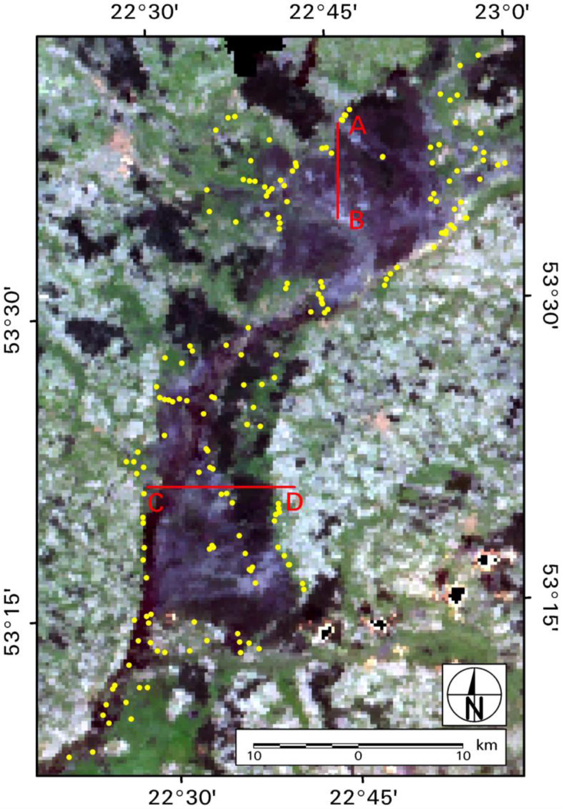
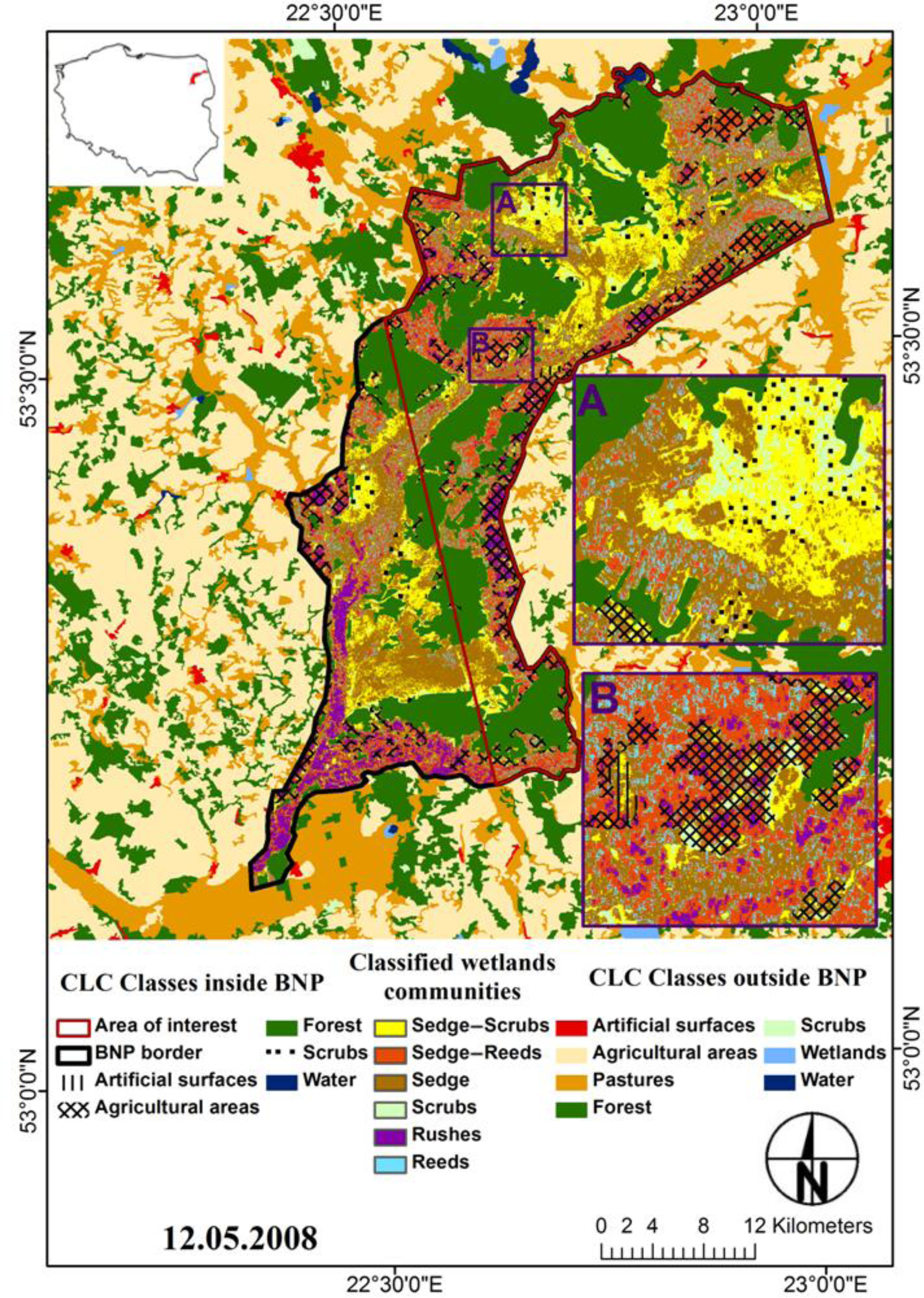
The study was conducted during the years of 2002–2010 in the Biebrza Wetlands situated in Northeast Poland on the Biebrza River Valley in the Podlaskie Voivodeship administrative division. The test site belongs to the Biebrza National Park (BNP) which was established in 1993 with a total area of 59,233 ha. The BNP includes 15,547 ha of forests, 18,182 ha of agricultural land, and 25,494 ha of peatlands—the most valuable habitats in the park [3]. Unique in Europe for its marshes and peat areas, as well as its many biodiversity rich plant habitats and highly diversified fauna, especially birds, BNP was designated as a wetland site of global significance at NATURA 2000 and since 1995 is under the protection of the RAMSAR Convention.
Both drying and moorsh-forming (peat degradation) processes occur on a large scale in the Biebrza Valley, mainly due to anthropogenic drainage and fluviogenic feeding limitation. Information about wetlands vegetation habitats and theirs biophysical properties derived from satellite images enable improvements in monitoring and managing areas that are very often impenetrable for ground truth observations. Satellite images registered in an optical spectrum are generally preferred for mapping of wetland vegetation habitats. Classification of wetland habitats using optical satellite data is difficult because of the spectral confusion between land cover classes especially among different types of wetlands. However, multi-temporal data usually improves the classification of wetlands, as well as ancillary data such as soil data, elevation or topography data [4]. Unfortunately, many wetlands areas are located in regions where cloud cover conditions exist. Since such conditions hinder the use of optical satellite images, many scientists suggested that microwave images could be an ideal tool for wetland habitats classification and calculation of biomass. Hess et al. [5] applied radar satellite data in L band to detect flooded areas beneath the forest canopy. These authors illustrated that L-band data provided clear distinction between flooded and non-flooded forest and between forest and marsh vegetation, although sometimes marsh vegetation had high returns that could be confused with flooded forest. Kasischke and Bourgeau-Chavez [6] used ERS-1 SAR (European Remote Sensing-1 Synthetic Aperture Radar, C-band) data for monitoring the presence or absence of water in wetlands. They have demonstrated that various vegetation communities could be distinguished based on canopy structure, soil moisture, and presence or absence of flooding. The authors indicated that generally the presence of water under a plant canopy increased the radar backscatter for wetlands with woody vegetation and decreased backscatter for wetlands with herbaceous vegetation. Townsend and Walsh [7] distinguished the difference between flooded and non-flooded areas on JERS-1 SAR (Japanese Earth Resources Satellite-1 Synthetic Aperture Radar, L-band) images. They demonstrated that ERS-1 SAR images were also useful for detecting the difference between flooded and non-flooded areas, although the differences were not as pronounced as on the JERS-1 SAR imagery. Kushwaha et al. [8] evaluated ERS-1 SAR and IRS-1B LISS-II (Indian Remote Sensing Satellite Linear Imaging Self-Scanning-II) data for discrimination of mangrove wetlands from other types of vegetation. They proposed a method that applies color composite images generated using either multi-temporal SAR data or by fusing SAR data with multispectral optical sensor data. Souza-Filho et al. [9] assessed the use of multi-polarized L-band airborne images for the identification of the Amazon coastal wetlands. They indicated that: HV polarization was the best for mapping abrupt boundaries in the coastal zone, such as those between mangroves and sand flats, and marshes and the coastal plateau, VV was the best for recognizing intertidal area morphology under low spring tide conditions, and HH was the best for mapping coastal environments covered with forest and scrub vegetation such as mangrove and vegetated dunes. Le Toan et al. [10] found that the best results have been noticed between HV polarization of L band and four forest variables: biomass, height, diameter at breast height and total stems.
The changes in soil moisture for the Biebrza Wetlands have been investigated by authors in previous study using radar data from ERS-1/2 SAR VV and ENVISAT ASAR HH (ENVIronmental SATellite Advanced Synthetic Aperture Radar) satellite images operating in C band. According to Dabrowska-Zielinska et al., both radar systems with a low incidence angle of the beam (23°) were suitable for delivering information on soil moisture [11].
As the importance of wetlands to the environment has become indisputable, there is an increasing need to monitor these valuable areas applying information derived from optical and radar satellite data for better conservation and management of wetland resources. In our investigations, such data come from satellites which exist or which will continue in orbit. The joint effect of applications of satellite data registering the reflected radiation in visible and infrared spectrums and thermal-infrared emitted radiation (ENVISAT MERIS—ENVIronmental SATellite MEdium Resolution Imaging Spectrometer, and NOAA AVHRR—National Oceanic and Atmospheric Administration Advanced Very High Resolution Radiometer), with the data from the active radar microwave spectrum (ALOS PALSAR—Advanced Land Observing Satellite Phased Array type L-band Synthetic Aperture Radar), has been used for this study to calculate the spectral reflectance, land-surface temperature, and backscattering coefficient of wetland areas. Although the ALOS satellite stopped working in April 2011, its successor, ALOS-2, will continue this mission with enhanced capabilities. The data obtained from optical and radar satellites provide the possibility to detect the changes in wetlands in different wave and spatial resolutions, store the processed data in the system that allows estimation of many biophysical parameters of the wetland ecosystem and then present this data spatially on maps. Among them, the most essential are vegetation cover (EO-based classification of wetland habitats), including its biomass and proxies of biomass such as LAI. LAI estimates are often used as surrogates for biomass in many vegetation growth models. This paper presents the methods for their assessment.
The goal of this study was to propose remote sensing methods for monitoring wetland ecosystems. To achieve this goal, satellite images acquired in optical and microwave spectrums were applied to address two objectives: (1) classification of wetlands habitats and the assessment of vegetation changes including area and biomass expressed by LAI using backscattering coefficient (σ°) calculated from PALSAR HV data; and (2) estimation of wetland biophysical properties such as moisture conditions expressed by surface temperature (Ts) calculated from AVHRR thermal channels and biomass expressed by Normalized Difference Vegetation Index (NDVI) calculated from MERIS red and near-infrared channels.
ENVISAT MERIS and ALOS PALSAR images have been obtained from ESA (European Space Agency) for AOALO.3742 and C1P.7389 projects, NOAA AVHRR images have been acquired by the station situated in the Institute of Geodesy and Cartography, and the land use cover outside the test site and forests areas were derived from CLC (Corine Land Cover) EU project.

2. Materials and Methods

2.1. Study Area

The Biebrza Wetlands belong to the largest National Park in Poland, which was created on 9 September 1993. It is located in Podlaskie Voivodeship, northeastern Poland, and is situated along the Biebrza River. The geographical position of the study area is: UL: 53°45′N, 22°15′E and LR: 53°10′N, 23°15′E. Figure 1 presents the area of the test site on the MERIS color composition RGB (Red-7, Green-5, Blue-2) image registered on 24 May 2010. Red lines represent localization of the two transects A–B and C–D for which chosen AVHRR data have been transformed into Ts and MERIS data into NDVI values. Yellow dots indicate localization of ground truth measurement points.
The study area is one of the largest inland wetlands in Europe and is still one of the wildest in Poland—not yet significantly affected by strong environmental or human disturbances. However, in recent decades, some attempts have been made to intensify and overexploit the natural resources of the region and implement new agriculture practices in the area. The canals that have been built disturbed the original water conditions and lowered the water table, which is most noticeable in the middle basin. The effect of lowering the water table was scrub encroachment, fires, and changes in farming activity. The farmers stopped cutting the grass when it became unprofitable under wetland conditions, and where it was not possible to do so using mechanical equipment. The advancing new vegetation encroachment caused biodiversity to decrease [1215]. BNP is now making various attempts towards re-naturalizing the area, such as organizing competitions in hand grass cuttings to protect the variety of plant species.
The Biebrza Wetlands are a flat area with an average altitude of about 105 m above sea level (a.s.l.). The altitude increases to the north, reaching approximately 120 m a.s.l. The main river is Biebrza, which flows out near the eastern border of Poland into the Narew River. The Biebrza drainage basin area is equal to 7051 km2, the river length is 155 km, and the mean flow amounts to 35.3 m3·s−1. The valley consists of mainly hydrogenic soils, with a dominant majority of peat soils in various stages of mouldering (decomposition). The spongy structure of the peat, which holds and stores liquids, makes the valley a huge reservoir of water [16]. The Biebrza Wetlands are flooded annually in the spring, which is the peat soils main water supply. These areas are mostly covered by sedges, reeds, rushes, moss, scrubs, grasses, and wildflower areas. The vegetation is characterized by great diversity, a high degree of naturalness and the presence of many rare species. The Biebrza Valley is naturally divided into three basins: the Upper Basin, the Middle Basin and the Lower Basin (the wettest one). In the Upper Biebrza Basin, the peat deposit is 3–6 m thick and covers an area of 14,000 ha. The Middle Basin has peat up to 3 m depth over an area of about 45,000 ha. Peatland in the Lower Biebrza Basin covers an area exceeding 23,000 ha with an average depth equal to 1.5 m [17].
The Biebrza Valley is one of the coolest regions in Poland—the mean year daily temperature equals 6.5 °C. The mean sum of yearly precipitation ranges from 550–650 mm and is one of the lowest in Poland. The length of the growing season is less than 200 days making it one of the shortest in Poland. Generally, summer is warm but short and winter is cold and long. The coldest month is January with a mean temperature of about −4.2 °C, and with temperatures dropping as low as −50 °C. Snow cover can last up to 140 days. July is the warmest month with mean temperatures of 17.5 °C, and with temperatures increasing up to 35.3 °C. The length of the summer ranges from 77–85 days [18].

2.2. Data Acquisition

2.2.1. In-Situ Data

In-situ data were collected during field campaigns carried out simultaneous to ALOS PALSAR satellite overpasses. The measurement sites were chosen within different wetland habitats and located on both sides of the Biebrza River (Figure 1). Although the number of chosen measurement points was equal to 150, only about half of them were visited during one five-day field campaign due to the large distances and accessibility (flooded). The geographic coordinates of the measurement plots were determined using a GPS receiver. This information was essential for the preparing of the special measurement points’ layers needed for the reading and processing of satellite data. The type of wetlands vegetation habitat, as well as vegetation development stages, have been described during each of the field campaigns.
The measurements of LAI were carried out with a LAI-2000 Plant Canopy Analyzer during each field campaign—the same sites were sampled three times. The area of LAI field measurements equals to about 60 × 60 m (5 × 5 ALOS pixels). Measurements have been spread around chosen points in order to calculate mean values for this site. A minimum of three observations have been taken around each of the measurement points which are marked as yellow dots on Figure 1. This device computes LAI from measurements made above and below the canopy, which are used to determine canopy light interception at five angles. These data are fit to a well-established model of radiative transfer inside vegetative canopies to compute LAI, mean tilt angle, and canopy gap fraction. The standard error of the LAI determinations (SEL) using LI-COR LAI-2000 Plant Canopy Analyzer at the 95% confidence level is within ±10% of true value. However, measurement error depends on many factors, such as the number of samples, sensor level, sky conditions and sensor set-up resolution; in our experience, the mean error was below 0.5 [19].
Meteorological data were collected from the meteorological station localized at the test site (in the Biebrza village, N53°39′ E22°32′) and from the closest station belonging to the national meteorological data network (in Bialystok city, 53°06′N, 23°10′E). During the years 2002–2010, meteorological conditions at the test site varied from extremely dry to very wet. The “dry years” were: 2002, 2003, 2005 and 2006 (the last one until August). The “wet years” were: 2004, 2008, and 2010. Vegetation hibernation conditions during winter and meteorological conditions in early spring also varied from year to year and are described in detail in this section. During winter time, the snow cover lingered at the test site in the years 2004–2008 and 2010 giving good hibernation conditions for vegetation and sufficient water retention in early springtime. The lack of water retention during early spring (April/May) occurred in the years 2002, 2003, 2006 and 2009 due to an insufficient amount of winter precipitation, which was considerably below the norm. The actual wetlands vegetation conditions depend mostly on soil moisture content. For the monitoring vegetation growth conditions, the amount of precipitation could be presumed to be a replacement in the absence of soil moisture data. The amount of precipitation during the early spring period (April/May) considerably exceeded the norm in the years 2004 and 2010. The air temperatures in the early spring (April/May) in the years 2005, 2006, 2008 and 2010 were much below the average for this period. Sunny and warm early spring has been observed in 2002, 2003 and 2009 with the mean air temperature much above the average for this period of time. Table 1 presents the accumulated values of air temperature and precipitation at the time of satellite images acquisition, i.e., at the third decade of April (Acc T1 and Acc P1) and at the first decade of May (Acc T2 and Acc P2) for the years 2002–2010. Table 1 shows that the highest accumulated values of air temperature calculated up to end of the first decade of May (Acc T2) occurred in the years 2002, 2003 and 2009. In the same periods, the accumulated values of precipitation were some of the lowest. In the year 2002, severe drought affected Poland. This analysis was derived on the basis of the observations of meteorological data collected at the station localized in Bialystok city.
Figure 2 presents the accumulated values of air temperature (Acc T) from the first decade of April until the third decade of September for the years 2002–2010 calculated using the mean daily data obtained from the “Biebrza village” meteorological station. Figure 3 presents the accumulated values of precipitation (Acc P) from the first decade of April until the third decade of September for the years 2002–2010 calculated using daily data from the same “Biebrza village” meteorological station. At the end of September, the highest accumulated values of air temperature (Figure 2) were observed for the years 2002–2004, while the lowest ones occurred in the year 2010. Considering accumulated values of precipitation (Figure 3), the highest values occurred in the year 2010, recognized as a “wet year”, while the lowest ones in the year 2002, recognized as a “dry year”.
Accumulated temperature and precipitation values are two of the most influential factors that determine vegetation growth and development and thus are very often used in models for biomass production assessment. Also, they can be used to estimate the heat stress on crops or for determination of harvest dates.

2.2.2. Satellite Data

For the investigation, the following satellite images have been used: level 1.5 ALOS PALSAR FBD (microwave, Fine Beam Dual Mode), ENVISAT MERIS FR (Full Resolution, visible and near-infrared), and NOAA AVHRR (thermal infrared). PALSAR provides an L-band SAR data at a high −12.5 m spatial resolution and almost monthly temporal resolution for all weather, day and night observations. PALSAR FBD is one of the five different science data modes in which PALSAR can operate with a polarization of HH/HV or VV/VH. MERIS is a medium-spectral resolution imaging spectrometer operating in 15 spectral bands in the range of 0.390–1.040 μm with a spatial resolution of 300 m at nadir and high temporal resolution (almost every day). AVHRR is a broad-band, five channel scanner sensing in the visible (two channels: 0.58–0.68 and 0.73–1.10 μm), near-infrared (3.55–3.93 μm) and thermal infrared (two channels: 10.30–11.30 and 11.50–12.50 μm) portions of the electromagnetic spectrum with the spatial resolution of 1100 m at nadir and every day registration. Chosen details of applied satellite images are presented in Table 2.
Microwave satellite images have been processed using ASF’s (Alaska Satellite Facility) MapReady Remote Sensing Tool Kit, and optical satellite images using ESA’s BEAM toolbox. MapReady is software for conversion synthetic aperture radar (SAR) and optical data in a variety of user friendly formats ready for additional processing, viewing or utilizing in GIS software. BEAM is a toolbox for viewing, analyzing and processing remote sensing raster data (including atmospheric corrections) developed to facilitate the utilization of image data from ENVISAT’s optical instruments. Complementarily, the ERDAS IMAGINE geospatial data system was used for: terrain geocoding; image classification; value readings around measurement points.
It was possible to obtain two PALSAR FBD registrations at HH- and HV-polarizations, with a 34.3 degree look angle for the study area for the dates 12 May 2008 and 1 May 2010 from which the backscattering coefficient (σ°) has been calculated. The readings of backscattering coefficient concern the window of 5 × 5 PALSAR pixels around a measurement point. To do this, Mean 5 × 5 filter existing in ERDAS system has been applied for previously filtered images (Speckle Filter: Local Region, window 7 × 7). From AVHRR images, the surface temperature (Ts) values were derived using channels 4 and 5 (10.30–11.30 and 11.50–12.50 μm, appropriately). From MERIS images, the NDVI values were calculated using channels 7 (red, 0.665 μm) and 13 (near-infrared, 0.865 μm).
Each satellite image has been rectified and transformed to the previously geometrically corrected (to the Polish CS92 map projection—EPSG projection 2180/ETRS89) panchromatic Landsat ETM+ image registered on 7 October 2000 for the CLC EU project. Topographic corrections of microwave images were not conducted because the study area is flat. Figures 4 and 5 present color compositions (Red, Green, Blue—RGB) of AVHRR and MERIS (appropriately) images acquired for the test site. Figure 6 presents a PALSAR FBD image registered in HV polarization.

2.3. Classification of Wetlands Vegetation Habitats

Depending on the frequency and polarization, the microwaves can penetrate through the vegetation into the soil. Backscatter and beam penetration vary due to different canopies, densities, and biomass. The longer the wavelength, the stronger the penetration into the soil [20]. According to Santoro et al. [21], who studied ALOS PALSAR data, better classification results are obtained from HV- than from HH- polarization. Cornforth et al. [22] illustrated the detection and mapping of mangroves based on ALOS PALSAR data. They found that HV polarization is more sensitive to vegetation structure and biomass than HH polarization. Whittle et al. [23] reported that detection of tropical deforestation using ALOS PALSAR HV data is only slightly better than with HH alone, and the best results are obtained by combining them. Although the papers presented above concern detection of clear-cuts or forest, these results are promising in classification of other vegetated areas including wetland ecosystems. Thus, we decided to apply ALOS PALSAR backscatter registered in long wave L at HV polarization for classification of wetlands vegetation habitats and for the assessment their changes. The obtained results presented here are consistent with the papers referred to previously.

2.4. Assessment of LAI

For proper management of wetland areas, it is necessary to provide regular satellite observations of LAI and biomass. Loss of vegetation cover expressed by LAI or biomass derived from satellite images indicates wetlands ecosystem degradation over time and area. This information presents a challenge to scientists and resource managers for better protection and conservation of wetlands. During cloudy conditions, the optical data could not be used, which is why applications of microwave data for the assessment of LAI have been tested using PALSAR images. Microwave images from PALSAR have been transformed to backscattering images in decibels (dB). The advanced radar sensor is a microwave instrument that transmits and receives signals to obtain high-quality images of the Earth’s surface in all weather conditions. The radar backscattering coefficient σ° is related to the radar brightness β° as follows [24]:
σ ° = β ° × sin α
where α is a local incident angle. The intensity values in PALSAR FBD products are directly proportional to the radar brightness β° of the illuminated scene.
For the study area, two PALSAR FBD registrations at HH- and HV-polarizations, with a 34.3 degree look angle, have been acquired for the dates 12 May 2008 and 1 May 2010. Calculated from the images, backscattering coefficient has been used along with ground truth observations of LAI in statistical analyses for the assessment of a relationship between these two variables. Then, for each of the classified wetlands habitats, different equations have been derived for the assessment of LAI values. Although these equations have been validated, additional corrections will be conducted using future PALSAR-2 data.

2.5. Calculation of Surface Temperature Ts and NDVI

The total emission from the soil-vegetation component is characterized by the radiances, which are received by the optical system of AVHRR in channels 4 and 5 (10.3–11.3 μm and 11.5–12.5 μm, appropriately). The radiances are calculated as follows [25]:
R 4 / 5 = G 4 / 5 × DN 4 / 5 + I 4 / 5
where: R4/5—radiance derived from channels 4 or 5, G4/5—slope value in channel 4 or 5, DN4/5—input digital number in channel 4 or 5, I4/5—intercept value in channel 4 or 5.
To convert radiances into top-of-atmosphere brightness temperatures the Planck function was used:
T = ( C 2 × ν ) / ( ln ( C 1 × ν 3 × R + 1 ) )
where: T—brightness temperature in Kelvin’s, C1,C2—Planck constants, ν—wave number of interest (in cm−1) in this case (4 or 5), and R—radiance.
To retrieve surface temperature (Ts) from the AVHRR top-of-atmosphere (TOA) brightness temperature (T) measurements, the “split window” algorithm has been applied [26]. The algorithm assumes that atmospheric attenuation (mostly due to atmospheric water vapor) is greater in channel 5 than in channel 4, and that the difference in measured radiance between these two channels increases with increasing water vapor. The best coefficients for Poland were used [27]. Then, surface temperature Ts has been corrected due to atmospheric influence as follows:
T s = T 4 + 2.68 ( T 4 T 5 ) 0.4
where: T4 and T5—brightness temperature in channels 4 and 5 (appropriately).
For the study, the mosaics of Ts representing two 10-day periods (third decade of April and at the first decade of May) have been done according to Kogan [28].
The Normalized Difference Vegetation Index (NDVI) is the most widely used index for remote sensing of vegetation in the past two decades. NDVI is calculated on the basis of spectral reflectance from the soil-vegetation surface acquired in the visible red (near 0.66 μm) and near infrared (around 0.86 μm) spectrum of electromagnetic wave according to [29]:
NDVI = ( NIR RED ) / ( NIR + RED )
where: RED—spectral reflectance in red spectrum and NIR—spectral reflectance in near-infrared spectrum. This index has been used in many applications, including estimating crop yields and end-of-season above-ground dry biomass [30].
The values of spectral reflectance are the ratios of the reflected over the incoming radiation in each spectral channel individually (albedo), hence they take on values between 0.0 and 1.0. In the present study, NDVI has been calculated using MERIS images acquired in channels 7 (red, 0.665 μm) and 13 (near-infrared, 0.865 μm). The following MERIS product has been used: MER_FR_1P. It is a Full-Resolution Geolocated and Calibrated TOA Radiance level 1 product. For atmospheric correction, the SMAC Processor (Simplified Method for Atmospheric Corrections), which is included in BEAM software, has been used. It is a semi-empirical approximation of the radiative transfer in the atmosphere. As the products from level 1 were applied, MERIS ECMWF (European Centre for Medium-Range Weather Forecasts) data for surface air pressure, ozone content and water vapor have been used.

3. Results and Discussion

For proper management of wetland ecosystems, it is important to know the location of and area occupied by particular vegetation communities, at which biomass (expressed by LAI) could be monitored by regular satellite observations. Usually, optical remote sensing data acquired with visible and near-infrared spectrum sensors are used for these purposes. However, during cloudy conditions such data are not available. In the present study, applications of microwave data for the classification of wetland communities and for the assessment of LAI have been tested using PALSAR images. Optical images registered by AVHRR and MERIS sensors have been used for Ts and NDVI calculations (appropriately).

3.1. Wetland Habitat Types Classification Using ALOS Microwave Images

The backscattering coefficients (σ°) calculated from PALSAR images registered at cross polarization HV on 12 May 2008 were used for the classification of main wetland communities. Image pixels were distributed between classes of wetland communities by setting thresholds on values of the backscattering coefficient. This procedure was conducted manually during visual interpretation according to information collected from the field survey. The maps prepared according to the above described approach can be treated as reliable and no additional verification was needed. Table 3 presents the values of the backscattering coefficient across the following six different vegetation classes: scrubs, sedges-scrubs, sedges, reeds, sedges-reeds and rushes.
The types of vegetation habitat were classified according to the backscattering values. The highest values of σ° occurred for scrubs (i.e., mean = −13.5 dB), whose vegetation surface roughness is high, the lowest σ° for rushes (i.e., mean = −30 dB), with a dense and smooth vegetation surface. Similar backscattering analysis is presented by Arnesen et al. [31]. They classified ALOS PALSAR ScanSAR HH backscatter into eight classes that were then split into three main groups as follows: forest cover types (flooded and non-flooded) with backscattering values higher than −8 dB, “Bright” areas (wet/rough soil, emergent macrophyte, rough open water) with backscattering values from −10 dB to −17.5 dB, and “Dark” areas (dry/smooth soil, floating macrophyte, smooth open water) with backscattering values from −19.5 dB to −24 dB.
The results of classification based on backscattering coefficient were laid on Corine Land Cover maps and presented in Figure 7. The same classification procedure has been adopted for the second PALSAR image registered two years later on 1 May 2010. On 1 May 2010, the south-west part of the test site was not covered with PALSAR satellite image (Figure 8). In order to detect changes in vegetation cover between these two dates of satellite acquisitions, only the areas that coincide on both images have been taken into consideration (Figures 7 and 8—red line). Then, both areas of each community and areas of changes of particular classes for both satellite acquisitions have been calculated. Table 4 displays the number of pixels and the area in hectares and in percentage of each vegetation class during both satellite acquisitions. As Table 4 shows, the largest area is occupied at both dates by the most typical wetland vegetation habitat—sedges, while the smallest one (besides scrubs on 12 May 2008) by rushes, which form the narrow strip close to the river beds or are situated in small local depressions. Comparing the area of each class for these two dates of satellite acquisitions separately, the largest changes appeared in the following classes: mixed sedges-reeds and scrubs. The area of sedges-reeds was reduced in 2010 due to the mowing practices of reeds embarked by BNP, and the area of scrubs increased in that year due to the scrub encroachment.
Table 5 displays the area of vegetation class cover changes in percentage, i.e., on what class the relevant class type existing in the year 2008 had been transformed in the year 2010. As Table 5 presents, the areas of reeds in the year 2008 had turned into sedges in more than 70% of the area in 2010. The rushes present a similar case—almost 31% had been turned into sedges and 41% into sedges-reeds. About 43% of sedges had been sprouted by scrubs and turned into mixed class sedges-scrubs. About 61% of sedges-reeds had been turned into sedges and almost 70% of sedges-scrubs into scrubs. These vegetation habitats changes are not seasonal as the dates of satellite acquisition concerned the same phenological stages of vegetation proved by analysis of meteorological data and seen in Table 1. These two-year vegetation community changes are due to BNP staff and service conservation, restoration and management activities.

3.2. Prediction of Leaf Area Index

Monitoring of wetland’s ecosystem including biomass expressed by LAI could be done by regular satellite radar observations. Wijaya et al. [32] studied tropical peatland regions using single and full polarimetry SAR data for modelling the biomass, LAI and tree age. They found the highest correlation between LAI and ALOS PALSAR backscatter for HV polarization and demonstrated that an exponential model of Polarimetry ALOS PALSAR data is more accurate than the polynomial model of ASAR. Canisius et al. [33] illustrated the relationship between LAI and both ALOS PALSAR L-band data and ENVISAT ASAR C-band data under relatively uniform soil moisture conditions. They determined that PALSAR L-band radar backscatter of crop (corn and soybean) fields and forest plots were in good agreement with measured LAI values while the C-band ASAR showed weak relationships. The strong positive correlation coefficients between the HV backscatter and LAI when the dead mangrove stands were considered have been indicated by Kovacs et al. [34]. However, significant negative values were calculated for the HH when dead mangrove stands were removed from the analysis. Xianfeng et al. [35] studied the sensitivity of multi-frequency (X, C and L-band) radar backscatter signatures to biophysical variables (LAI) over corn and soybean fields. The results of their study showed that the lower frequency bands, such as L and C, were closely related with LAI. For both corn and soybean crops, most C-band linear (HH, VV, HV) backscatter coefficients were correlated with LAI. L-band backscatter at HH and HV polarizations produced the highest correlations with corn LAI (r = 0.90–0.96), while only weak correlation with soybean LAI.
For the assessment of LAI, microwave PALSAR images have been applied in the present study. Backscattering coefficients (σ°) calculated from PALSAR FBD images registered in cross polarization HV on 12 May 2008 and 1 May 2010 were used in statistical analyses along with LAI ground truth observations carried out during satellite overpasses. These analyses have been performed for each of the wetland communities separately using STATISTICA software. As a result, the linear relationships between LAI and σ° have been derived for particular wetland classes at a 95% confidence level with the highest standard error of estimation equal to 0.57 LAI for the class sedges-reeds. Table 6 presents the results of these statistical analyses. Derived equations have been applied for selected measurement plots (taking into account all six habitats from Table 3) for the validation procedure (Figure 9). As Figure 9 shows, most of the LAI values are underestimated. The next validation procedure will be carried out in the future by applying new PALSAR-2 data (authors’ project accepted by JAXA—Japan Aerospace Exploration Agency) and derived equations, which are highly dependent on the accuracy of classification of wetlands habitats, to correct these values.
The equations obtained based on the statistical analyses between LAI and backscattering coefficients (Table 6) were used to elaborate the maps of LAI for wetlands communities. PALSAR HV images registered on 12 May 2008 and 1 May 2010 were processed and transformed to LAI maps (Figures 10 and 11). LAI values have been grouped into the following six classes: <1; 1–2; 2–3; 3–4; 4–5; 5–6. As can be seen on these maps, the LAI values on 1 May 2010 were higher than on 12 May 2008 due to a higher amount of precipitation (see Subsection 2.2.1) and better temperature conditions for vegetation growth.
In order to compare changes of LAI values derived from both PALSAR acquisitions, the area occupied by each of the LAI classes has been calculated. Table 7 shows the obtained results. The largest area belongs to LAI classes 3–4 and 4–5, while the lowest to classes <1 and 5–6 in the year 2008 and to class <1 in the year 2010. Generally, in the year 2010, the largest area with high LAI values (>4) and the smallest one with low LAI values (<2) occurred. The average LAI values calculated for each of the classified wetlands communities, applying equations from Table 6, have been plotted against average σ° values (scrubs: −13.5, sedges-scrubs: −17.5, sedges: −21.5, reeds: −24.5, sedges-reeds: −26.5 and rushes: −30) (Figure 12 presents this relationship). The obtained relationship shows that with the increase of LAI there is an increase in the backscattering coefficient, which indicates the strong possibilities to monitor the increase of biomass using the long L wave of PALSAR data [10,36]. The relationship between LAI and biomass, which is strong for wetland vegetation habitats, has been elaborated by authors in previous studies and is described in papers [3638].

3.3. Ts and NDVI—Application of Optical Images

Thermal infrared channels (4, 5) of AVHRR images have been applied for the calculation of surface temperature—Ts (see Subsection 2.5). It was assumed that the surface temperature characterizes the vegetation growth conditions well. Calculated values of Ts were presented on the maps. Figures 13 and 14 show the surface temperature distribution at the test site for the turn of April/May in the years 2003 (dry season) and 2008 (wet season), overlaid on the CLC classes. For the largest part of the test site in the year 2003, the values are in the range of 25–30 °C, (Figure 13), while in 2008 the surface temperature is in the range of 15–20 °C, (Figure 14). These almost twofold differences reflect observed weather conditions—the year 2008 has been noted as a year with a cold, early spring with the mean amount of precipitation for April/May, while the year 2003 was warm and dry (see Subsection 2.2.1). It was also observed that in the year 2003 there is a great difference between the temperature of the forest, marshland and pastures, while for the year 2008 there is no large difference in temperature for various communities. This indicates that in humid areas—such as wetlands—for different vegetation cover, air temperature was higher (see Table 1) than surface temperature, which caused higher evapotranspiration in 2003 than in April/May 2008, and much higher variation between different vegetation communities. Detailed information of Ts values within the classified vegetation communities (see Table 3) has been extracted for two transects A–B (Middle Basin) and C–D (Lower Basin), (see Figure 1) and displayed on the graphs. Figures 15 and 16 show values of Ts along both transects extracted for the turn of April/May in the years 2003, 2006, 2008 and 2010. The highest values of Ts in that period have been observed in the years 2003 and 2006 for the sedges-reeds and sedges-scrubs classes, while the lowest ones were observed in the years 2008 and 2010.
It is also interesting that there were large differences between surface temperature Ts in 2003 and 2006 and in 2008 and 2010 for the A–B transect in the Middle Basin (Figure 15). For the southern part of the Lower Basin of Biebrza (transect C–D), the temperatures of 2003 and 2006 were also higher than in 2008 and 2010 but the difference was not so significant (Figure 16). The southern part of the Lower Basin (C–D transect) is much wetter than the Middle Basin (transect A–B). The changes in vegetation communities happen more quickly (see Subsection 2.1). In general, surface temperature characterizes moisture and evapotranspiration conditions. The classes along the transects of the X-axis in Figures 15 and 16 are reliable for the years 2008–2010 for which habitat classification has been carried out. The graphs for the years 2003 and 2006 are presented just to show the differences in Ts values caused by variations in each Basin’s moisture and weather conditions.
The next procedure was the application of channels 13 (near-infrared) and 7 (red) of MERIS images for calculation of NDVI index (see Subsection 2.5). Here, detailed information of NDVI values within classified vegetation communities (see Table 3) has also been extracted for the same two transects A–B and C–D (see Figure 1) and displayed on the graphs (Figures 17 and 18). Figures 17 and 18 present the values of NDVI along the both transects extracted for the turn of April/May in the years 2003, 2006, 2008 and 2010. Here also, (as for Figures 15 and 16) the classes along transects of the X-axis in Figures 17 and 18 are reliable for the years 2008–2010 for which habitat classification has been carried out. The graphs for the years 2003 and 2006 are presented just to show differences in NDVI values caused by variations in Basins moisture and weather conditions. The lowest NDVI values have been observed in the year 2006, which was considered the year with a cold and dry spring. The highest values of NDVI occurred in 2008 and 2010, which were distinguished as cold years but with sufficient amounts of precipitation. The year 2003, for most communities, was dry as reflected in lower NDVI values. Differences of NDVI values within the same class resulted mainly from differences in soil moisture that could have an impact on vegetation density, which is represented by NDVI. Thus, it is difficult to attribute exact NDVI values for particular classes. However, NDVI index calculated from MERIS images could be used for biomass assessment as indicated by authors in previous studies and is described in papers [3941].

4. Conclusions

The main purpose of this study was to present the methods based on optical and radar satellite data for monitoring the environmental conditions of the inland wetland ecosystems. To achieve this objective, application of various satellite images registered in the optical spectrum as visible, infrared, and thermal-infrared data and in the microwave spectrum as L-band data was proposed to estimate significant biophysical variables such as T
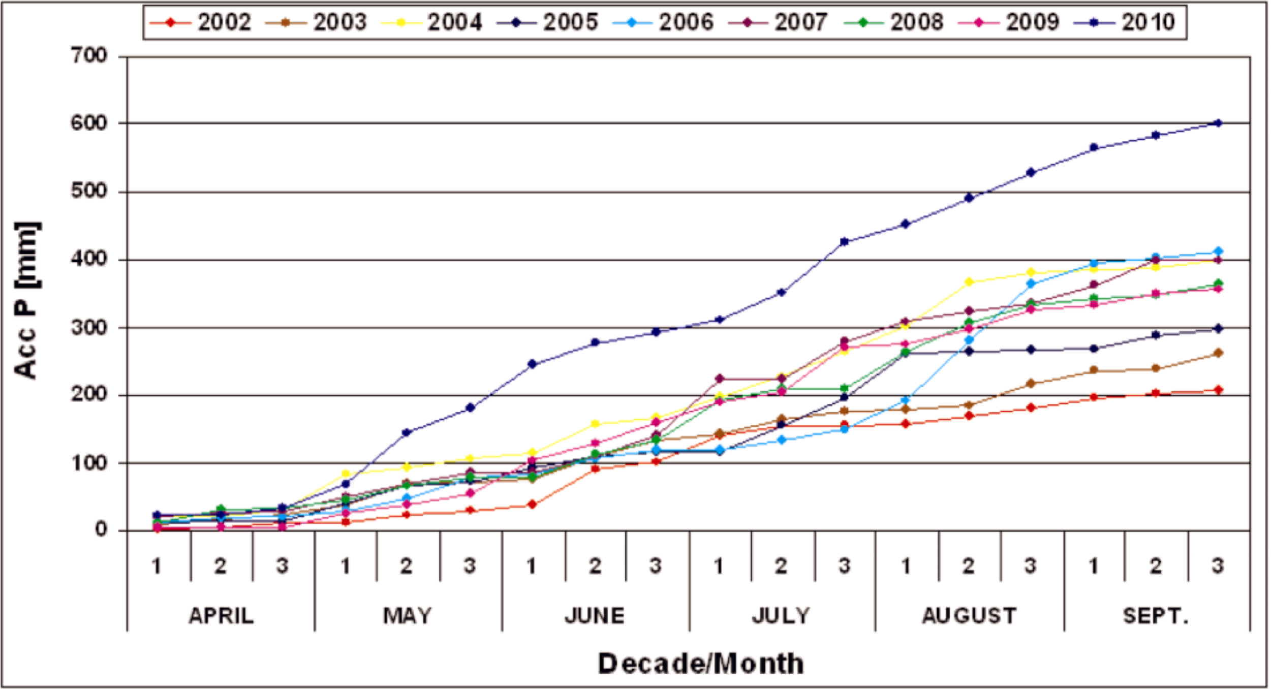
s (surface temperature), NDVI (Normalized Difference Vegetation Index) and LAI (Leaf Area Index) that describe well the complex spatio-temporal patterns of wetland ecosystem conditions. For the years 2002–2010, it was possible to attain the optical data from the high temporal resolution (everyday registration) NOAA AVHRR (National Oceanic and Atmospheric Administration Advanced Very High Resolution Radiometer) satellite. The soil and vegetation conditions during the NOAA AVHRR data registrations were characterized by different climatic conditions with four dry (2002, 2003, 2005 and 2006) and three wet (2004, 2008 and 2010) years. However, these satellite images have a spatial resolution of 1100 m, which was too low to classify the vegetation communities. We used high spatial resolution (but low temporal resolution) Landsat +ETM (Enhanced Thematic Mapper Plus), ALOS AVNIR-2 (Advanced Land Observing Satellite, Advanced Visible and Near Infrared Radiometer) and Terra ASTER (Advanced Spaceborne Thermal Emission and Reflection Radiometer), as well as medium resolution ENVISAT MERIS (ENVIronmental SATellite MEdium Resolution Imaging Spectrometer) satellite images, for the classification of wetland’s vegetation habitats in our previous study [11,36,37]. The results were satisfying as satellite images registered in the optical spectrum are widely used for land use/land cover mapping. However, in the current investigation, we applied microwave data that can potentially detect different types of wetland habitats and can be used to study the conditions and functions of these areas independently of cloudy conditions. The dependence of radar backscatter on water content, due to its high dielectric constant, is crucial for wetland examination. Thus, we used high resolution ALOS PALSAR images (Advanced Land Observing Satellite, Phased Array type L-band Synthetic Aperture Radar). The data from the ALOS PALSAR satellite were obtained only for the years 2008 and 2010 for two dates covering the beginning of growing season. Backscattering coefficients calculated from these images were applied for the classification of wetland habitats and calculation of LAI with good results. The six wetland habitats have been distinguished and strong relationships between LAI and σ° values have been derived and validated.
The problem of scrub development in wetland areas—being a threat for the protected wetland vegetation—can be monitored by applying L-band with HV polarization and a large incidence angle of the radar beam. The scrubs have the largest biomass and the process of scrub encroachment can be well monitored by the highest values of radar backscattering coefficients. The good relationship obtained between backscattering coefficients and LAI shows that long wave (L) with HV polarization and a large incidence angle (38.7°) of PALSAR wave could be used for wetland vegetation LAI estimates. This indicates the strong possibilities to monitor changes in biomass using low frequency, cross-polarized HV SAR (Synthetic Aperture Radar) data.
Use of thermal-infrared data from AVHRR images allows monitoring the surface temperature, which represents, to a large extent, moisture conditions. The application of meteorological data, measured at the same time as satellite acquisitions, will allow estimation of the sensible heat fluxes and further latent heat fluxes characterizing the evapotranspiration conditions. The NDVI index calculated from MERIS images could be used for LAI and then for biomass assessment and monitoring changes.
Mapping and monitoring wetlands using remote sensing methods presents a challenge to scientists and resource managers for which the provision of relevant, compatible data and information is necessary. The proposed methodology could be used as the baseline for ecological monitoring and assessment of environmental conditions of wetland ecosystems in other parts of Europe because the studied area can be recognized as a reference for other lowland river valley wetlands.
The future system for monitoring changes in the wetlands’ ecosystem should be based on both optical and radar data supported by in-situ measurements. In the year 2014, the new ALOS-2 satellite will be launched by JAXA (Japan Aerospace Exploration Agency, Tokyo, Japan). The European satellites Sentinel-1/2 will be launched in 2014 within the GMES/Copernicus program. The authors have projects accepted by JAXA and ESA (European Space Agency, Paris, France) that will allow the possibility to use the synergy of microwave and optical data for monitoring wetland environmental conditions and their changes with high spatial and temporal resolution. It will be very important to use multi-polarized radar data from ALOS-2 and Sentinel-1 and optical data from Sentinel-2 to differentiate between the biomass of the wetland’s habitats and to develop an operational monitoring system of the wetland’s environmental changes.

Acknowledgments

The research has been done within the National Project No. N N526 160040. We gratefully acknowledge ESA for providing ENVISAT and ALOS images for the Projects: AOALO.3742 and C1P.7389.

Author Contributions

All authors have been engaged in field campaigns and additionally:
Katarzyna Dabrowska-Zielinska—overall conception of the study and article, writing; Maria Budzynska—statistical analyses, validation, writing, revisions; Monika Tomaszewska—visual classification of ALOS PALSAR images, preparation maps of wetland communities, calculation of area in hectares and in percentage of each class, calculation of class cover area changes, preparation of maps of LAI distribution; Maciej Bartold—processing of NOAA AVHRR data, calculation of surface temperature (Ts), elaboration of Ts maps and transects; Martyna Gatkowska—processing of in-situ measurements, database set up and maintenance; Iwona Malek—processing of ALOS PALSAR data, preparation of measurement points layer, preparation of CLC layers, calculation and readings of backscattering coefficient; Konrad Turlej—processing of ENVISAT MERIS data, calculation of NDVI, elaboration of NDVI transects; Milena Napiorkowska—processing and analyses of meteorological data, calculation of accumulated values of air temperature and precipitation and elaboration of graphs.

Conflicts of Interest

The authors declare no conflict of interest.

References

  1. Mitsch, W.J.; Gosselink, J.G. The Value of wetlands: Importance of scale and landscape setting. Ecol. Econ 2000, 7, 25–33. [Google Scholar]
  2. Rodriguez-Iturbe, I.; Porporato, A. Introduction. In Ecohydrology of Water-Controlled Ecosystems: Soil Moisture and Plant Dynamics; Cambridge University Press: Cambridge, UK, 2004; pp. 6–7. [Google Scholar]
  3. Biebrza National Park. Available online: http://www.biebrza.org.pl/14,biebrzanski-pn.html (accessed on 24 March 2009).
  4. Ozesmi, S.L.; Bauer, M.E. Satellite remote sensing of wetlands. Wetl. Ecol. Manag 2002, 10, 381–402. [Google Scholar]
  5. Hess, L.L.; Melack, J.M.; Simonett, D.S. Radar detection of flooding beneath the forest canopy: A review. Int. J. Remote Sens 1990, 11, 1313–1325. [Google Scholar]
  6. Kasischke, E.S.; Bourgeau-Chavez, L.L. Monitoring South Florida wetlands using ERS-1 SAR imagery. Photogramm. Eng. Remote Sens 1997, 63, 281–291. [Google Scholar]
  7. Townsend, P.A.; Walsh, S.J. Modeling floodplain inundation using an integrated GIS with radar and optical remote sensing. Geomorphology 1998, 21, 295–312. [Google Scholar]
  8. Kushwaha, S.P.S.; Dwivedi, R.S.; Rao, B.R.M. Evaluation of various digital image processing techniques for detection of coastal wetlands using ERS-1 SAR data. Int. J. Remote Sens 2000, 21, 565–579. [Google Scholar]
  9. Souza-Filho, P.W.M.; Paradella, W.R.; Rodrigues, S.W.P.; Costa, F.R.; Mura, J.C.; Gonçalves, F.D. Discrimination of coastal wetland environments in the Amazon region based on multi-polarized L-band airborne Synthetic Aperture Radar imagery. Estuar. Coast. Shelf Sci 2011, 95, 88–98. [Google Scholar]
  10. Le Toan, T.; Beaudoin, A.; Riom, J.; Guyon, D. Relating forest biomass to SAR data. IEEE Trans. Geosci. Remote Sens 1992, 30, 403–411. [Google Scholar]
  11. Dabrowska-Zielinska, K.; Gruszczynska, M.; Lewinski, S.; Hoscilo, A.; Bojanowski, J. Application of remote and in situ information to the management of wetlands in Poland. J. Environ. Manag 2009, 90, 2261–2269. [Google Scholar]
  12. Byczkowski, A.; Okruszko, T. Restoration of protected fenlands (case study for the central basin of the Biebrza River Valley). Rocz. Akad. Rol. Pozn 2004, 25, 15–21. [Google Scholar]
  13. Klosowski, T. Biebrza Marshland; Janudi, M., Ed.; VOUAGER: Warsaw, Poland, 1994. [Google Scholar]
  14. Kundzewicz, Z.W. Ecohydrology for Sustainable Wetlands under Global Change—Data, Models, Management. In Measurement Techniques and Data Assessment in Wetlands Hydrology; Ignar, S., Nowakowski, P., Okruszko, T., Eds.; Warsaw Agricultural University Press: Warsaw, Poland, 2003; pp. 25–35. [Google Scholar]
  15. Zurek, S. Rzezba i Budowa Geologiczna Doliny Biebrzy. In Przyroda Biebrzanskiego Parku Narodowego; Dyrcz, A., Werpachowski, C., Eds.; Biebrzanski Park Narodowy Press: Osowiec-Twierdza, Poland, 2005; pp. 19–32. [Google Scholar]
  16. Sienko, A.; Grygoruk, A. Biebrzanski Park Narodowy. In Biebrzanski Park Narodowy; Sienko, A., Grygoruk, A., Eds.; Biebrzanski Park Narodowy Press: Osowiec-Twierdza, Poland, 2003; pp. 10–12. [Google Scholar]
  17. Dembek, W.; Oswit, J.; Rycharski, M. Torfowiska i Torfy w Pradolinie Biebrzy. In Przyroda Biebrzanskiego Parku Narodowego; Dyrcz, A., Werpachowski, C., Eds.; Biebrzanski Park Narodowy Press: Osowiec-Twierdza, Poland, 2005; pp. 33–58. [Google Scholar]
  18. Silakowski, M. Charakterystyka Fizyczno-Geograficzna-Klimat. In Biebrzanski Park Narodowy; Sienko, A., Grygoruk, A., Eds.; Biebrzanski Park Narodowy Press: Osowiec-Twierdza, Poland, 2003; pp. 17–22. [Google Scholar]
  19. LI-COR Inc. LAI-2000 Plant Canopy Analyzer; LI-COR Inc.: Lincoln, NE, USA, 1992. [Google Scholar]
  20. SAR-Guidebook, 1.4 Scattering Mechanisms. Available online: http://www.sarmap.ch/pdf/SAR-Guidebook.pdf (accessed on August 2009).
  21. Santoro, M.; Pantze, A.; Fransson, J.E.S.; Dahlgren, J.; Persson, A. Nation-wide clear-cut mapping in Sweden using ALOS PALSAR strip images. Remote Sens 2012, 4, 1693–1715. [Google Scholar]
  22. Cornforth, W.A.; Fatoyinbo, T.E.; Freemantle, T.P.; Pettorelli, N. Advanced land observing satellite phased array type L-band SAR (ALOS PALSAR) to inform the conservation of mangroves: Sundarbans as a case study. Remote Sens 2013, 5, 224–237. [Google Scholar]
  23. Whittle, M.; Quegan, S.; Uryu, Y.; Stuewe, M.; Yulianto, K. Detection of tropical deforestation using ALOS-PALSAR: A Sumatran case study. Remote Sens. Environ 2012, 124, 83–98. [Google Scholar]
  24. Laur, H.; Bally, P.; Meadows, P.; Sanchez, J.; Schaettler, B.; Lopinto, E.; Esteban, D. Derivation of the Backscattering Coefficient Sigma-Nought in ESA ERS SAR PRI Products; European Space Agency: Rome, Italy, 1998. [Google Scholar]
  25. NOAA Polar Orbiter Data User’s Guide. Available online: http://www.ncdc.noaa.gov/oa/pod-guide/ncdc/docs/podug/html/c3/sec3-3.htm (accessed on 17 December 2003).
  26. Coll, C.; Caselles, V. A split-window algorithm for land surface temperature from advanced very high resolution radiometer data: Validation and algorithm comparison. J. Geophys. Res 1997, 102, 16697–16713. [Google Scholar]
  27. Dabrowska-Zielinska, K.; Gruszczynska, M.; Lewinski, S. Soil Moisture in the Root Zone of Vegetation Determined from AVHRR/NOAA Satellite. Proceedings of 12th Remote Sensing for Monitoring the Changing Environment of Europe Symposium, Eger, Hungary, 8–11 September 1992.
  28. Kogan, F.N. Global drought watch from space. Bull. Am. Meteorol. Soc 1997, 78, 621–636. [Google Scholar]
  29. Tucker, C.J. Red and photographic infrared linear combinations for monitoring vegetation. Remote Sens. Environ 1979, 8, 127–150. [Google Scholar]
  30. Tucker, C.J.; Justice, C.O.; Pince, S.D. Monitoring the grasslands of the Sahel 1984–1985. Int. J. Remote Sens 1986, 7, 1571–1581. [Google Scholar]
  31. Arnesen, A.; Silva, T.S.F.; Hess, L.L.; Novo, E.; Rudorff, C.M. Monitoring flood extent in the lower Amazon River floodplain using ALOS/PALSAR ScanSAR images. Remote Sens. Environ 2013, 130, 51–61. [Google Scholar]
  32. Wijaya, A.; Susanti, A.; Liesenberg, V.; Wardhana, W.; Yanto, E.; Soeprijadi, D.; Mc Farlane, C.; Qomar, N. Leaf Area Index and Biomass Assessment over Tropical Peatland Forest Ecosystem Using ALOS Palsar and ENVISAT ASAR Data. Proceedings of the 5th International Workshop on Science and Applications of SAR Polarimetry and Polarimetric Interferometry, Frascati, Italy, 24–28 January 2011.
  33. Canisius, F.; Fernandes, R. ALOS PALSAR L-band polarimetric SAR data and in situ measurements for leaf area index assessment. Remote Sens. Lett 2012, 3, 221–229. [Google Scholar]
  34. Kovacs, J.M.; Lu, X.X.; Flores-Verdugo, F.; Zhang, C.; Flores de Santiago, F.; Jiao, X. Applications of ALOS PALSAR for monitoring biophysical parameters of a degraded black mangrove (Avicennia germinans) forest. ISPRS J. Photogramm. Remote Sens 2013, 82, 102–111. [Google Scholar]
  35. Xianfeng, J.; McNairn, H.; Shang, J.; Liu, J. The Sensitivity of Multi-Frequency (X, C and L-band) Radar Backscatter Signatures to Bio-Physical Variables (LAI) over Corn and Soybean Fields. Proceeding of ISPRS TC VII Symposium—100 Years ISPRS, Vienna, Austria, 5–7 July 2010; Wagner, W., Székely, B., Eds.; IAPRS: Vienna, Austria, 2010. [Google Scholar]
  36. Dabrowska-Zielinska, K.; Budzynska, M.; Kowalik, W.; Malek, I.; Gatkowska, M.; Bartold, M.; Turlej, K. Biophysical parameters assessed from microwave and optical data. Int. J. Electron. Telecom 2012, 58, 99–104. [Google Scholar]
  37. Budzynska, M.; Dabrowska-Zielinska, K.; Turlej, K.; Malek, I.; Bartold, M. Monitoring of the Biebrza Wetlands using remote sensing methods. Water Environ. Rural Areas 2011, 11, 65–72. [Google Scholar]
  38. Dabrowska-Zielinska, K.; Budzynska, M. Monitoring Wetlands Area Using Microwave, Optical and In-Situ Data. Proceedings of the ESA eLEAPS EGU Earth Observation for Land-Atmosphere Interaction Science, Rome, Italy, 3–5 November 2010.
  39. Dabrowska-Zielinska, K.; Budzynska, M.; Kowalik, W.; Malek, I.; Turlej, K.; Bochenek, Z. Soil moisture and evapotranspiration of wetlands vegetation habitats retrieved from satellite images. Hydrol. Earth Syst. Sci 2010, 7, 5929–5955. [Google Scholar]
  40. Dabrowska-Zielinska, K.; Budzynska, M.; Kowalik, W.; Malek, I.; Turlej, K. Characterizing Status of Selected Ecosystems Using Optical and Microwave Remote Sensing Data. Proceedings of the ESA Living Planet Symposium, Bergen, Norway, 28 June–2 July 2010.
  41. Dabrowska-Zielinska, K.; Budzynska, M.; Kowalik, W.; Malek, I.; Turlej, K. Study in Biebrza Wetlands Using Optical and Microwave Satellite Data. Proceedings of the 2010 IEEE International Geoscience and Remote Sensing Symposium, Honolulu, HI, USA, 25–30 July 2010.
Figure 1. Test site on MERIS RGB (7, 5, 2) composition with transects A–B and C–D marked by the red line for which chosen AVHRR data have been transformed into Ts and MERIS data into NDVI values.
Remotesensing 06 01605f1
Figure 2. Accumulated values of air temperature (Acc T).
Remotesensing 06 01605f2
Figure 3. Accumulated values of precipitation (Acc P).
Remotesensing 06 01605f3
Figure 4. Red, Green, Blue (RGB) (4, 2, 1) composition of AVHRR image acquired on 24 April 2008.
Remotesensing 06 01605f4
Figure 5. RGB (10, 5, 3) composition of MERIS image acquired on 25 April 2010.
Remotesensing 06 01605f5
Figure 6. PALSAR FBD HV image acquired on 12 May 2008.
Remotesensing 06 01605f6
Figure 7. Map of wetland communities classified based on PALSAR HV image registered on 12 May 2008, placed on CLC classes.
Remotesensing 06 01605f7
Figure 8. Map of wetland communities classified based on PALSAR HV image registered on 1 May 2010, placed on CLC classes.
Remotesensing 06 01605f8
Figure 9. Plot of the LAI measured versus estimated from PALSAR HV images.
Remotesensing 06 01605f9
Figure 10. Map of LAI distribution on 12 May 2008 within the area of interest.
Remotesensing 06 01605f10
Figure 11. Map of LAI distribution on 1 May 2010 within the area of interest.
Remotesensing 06 01605f11
Figure 12. Relationship between mean σ° (sigma) and mean LAI for wetland habitats.
Remotesensing 06 01605f12
Figure 13. Surface temperatures at the test site at the turn of April/May 2003 (dry season).
Remotesensing 06 01605f13
Figure 14. Surface temperatures at the test site at the turn of April/May 2008 (wet season).
Remotesensing 06 01605f14
Figure 15. Ts along the transect A–B calculated from AVHRR images.
Remotesensing 06 01605f15
Figure 16. Ts along the transect C–D calculated from AVHRR images.
Remotesensing 06 01605f16
Figure 17. NDVI values along the transect A–B calculated from MERIS images.
Remotesensing 06 01605f17
Figure 18. NDVI values along the transect C–D calculated from MERIS images.
Remotesensing 06 01605f18
Table 1. Accumulated values of air temperature and precipitation during the third decade of April (Acc T1, Acc P1) and the first decade of May (Acc T2, Acc P2) for the years 2002–2010.
YearAcc T1 (°C)Acc T2 (°C)Acc P1 (mm)Acc P2 (mm)
200224941511.111.1
200329146222.937.2
200421634731.783.1
20051972411440.3
200618327719.528.6
200727034730.149.7
200815523633.845.7
20092963954.524.4
20101912253466.4
Table 2. Selected details of satellite data applied for the investigation.
Satellite SensorSpatial Resolution (m)Polarization Spectral RangeIncidence Angle (°)
ALOS PALSAR12.5HV, L (23.62 cm, 1.27 GHz)38.7
ENVISAT MERIS300 at nadir0.39–1.04 μmnadir
NOAA AVHRR1100 at nadir0.58–12.50 μmnadir
Table 3. Values of σ° and corresponding classes of wetland communities.
σ° Values (dB)Class Name
from −11 to −16Scrubs
from −16 to −19Sedges-Scrubs
from −19 to −24Sedges
from −24 to −25Reeds
from −25 to −28Sedges-Reeds
from −28 to −32Rushes
Table 4. The number of pixels and area in hectares and in percentage of each class.
DateClass NameNumber of PixelsArea (ha)Area (%)
12 May 2008Scrubs139,4282178.564.54
Sedges-Scrubs560,0748751.1618.24
Sedges991,82115,497.2032.30
Reeds305,1864768.539.94
Sedges-Reeds896,60514,009.4529.20
Rushes177,5162773.695.78

1 May 2010Scrubs691,23310,800.5222.59
Sedges-Scrubs657,07210,266.7521.47
Sedges1,220,95919,077.4839.89
Reeds243,5353805.237.96
Sedges-Reeds241,5593774.367.89
Rushes619296.750.20
Table 5. Class cover area changes in percentage.
2010/2008ScrubsSedges&ScrubsSedgesReedsSedges&ReedsRushes
Scrubs89.7769.6316.751.800.390.03
Sedges-Scrubs3.8326.7043.2713.103.640.28
Sedges1.003.1937.8073.7560.9431.26
Reeds0.020.041.417.6018.0325.08
Sedges-Reeds0.010.030.683.7016.8041.04
Rushes0.000.000.020.020.202.30
Unclassified5.360.410.080.020.010.00
Table 6. Results of the statistical analyses between LAI and σ° at a 95% confidence level.
Class NameR2 (%)Number of ObservationsStandard Error of Est.Equation
Scrubs84.81200.13LAI = 0.24σ° + 8.06
Sedges-Scrubs72.74290.45LAI = 0.34σ° + 10.58
Sedges81.61250.30LAI = 0.35σ° + 11.35
Reeds79.77220.46LAI = 1.12σ° + 28.86
Sedges-Reeds74.70260.57LAI = 0.57σ° + 17.87
Rushes78.79210.35LAI = 1.27σ° + 39.89
Table 7. Number of pixels and area in hectares and in percentage of particular LAI classes.
DateLAINumber of PixelsArea (ha)%
12 May 2008<141,609650.141.36
1–2295,8584622.789.64
2–3560,4918757.6718.25
3–41,037,34316,208.4833.78
4–51,083,08016,923.1335.27
5–652,244816.311.70

1 May 2010<126,155408.670.85
1–2219,4003428.137.17
2–3117,8121840.813.85
3–4951,64214,869.4131.09
4–51,545,53724,149.0250.50
5–6200,0033125.056.53

