Article

Characterizing the Spatial Structure of Mangrove Features for Optimizing Image-Based Mangrove Mapping

1
Biophysical Remote Sensing Group, School of Geography, Planning and Environmental Management, The University of Queensland, Brisbane, QLD 4072, Australia
2
Cartography and Remote Sensing Study Program, Faculty of Geography, Gadjah Mada University, Bulaksumur, Yogyakarta 55281, Indonesia
*
Author to whom correspondence should be addressed.
Remote Sens. 2014, 6(2), 984-1006; https://doi.org/10.3390/rs6020984
Submission received: 25 November 2013 / Revised: 20 December 2013 / Accepted: 14 January 2014 / Published: 27 January 2014

Abstract

:
Understanding the relationship between the size of mangrove structural features and the optimum image pixel size is essential to support effective mapping activities in mangrove environments. This study developed a method to estimate the optimum image pixel size for accurately mapping mangrove features (canopy types and features (gaps, tree crown), community, and cover types) and tested the applicability of the results. Semi-variograms were used to characterize the spatial structure of mangrove vegetation by estimating the size of dominant image features in WorldView-2 imagery resampled over a range of pixel sizes at several mangrove areas in Moreton Bay, Australia. The results show that semi-variograms detected the variations in the structural properties of mangroves in the study area and its forms were controlled by the image pixel size, the spectral-band used, and the spatial characteristics of the scene object, e.g., tree or gap. This information was synthesized to derive the optimum image pixel size for mapping mangrove structural and compositional features at specific spatial scales. Interpretation of semi-variograms combined with field data and visual image interpretation confirms that certain vegetation structural features are detectable at specific scales and can be optimally detected using a specific image pixel size. The analysis results provide a basis for multi-scale mangrove mapping using high spatial resolution image datasets.

1. Introduction

Remote sensing has been used extensively to map and monitor mangrove environments over the past two decades. It offers some key advantages for mangrove studies, including indirect access to mangrove habitats that are usually hard to access [1,2], extrapolation of observation results at specific sample sites over large areas [3], and delivery of data at specific spatial and temporal scales [4]. Recent developments in remote sensing and image processing allow us to explore various types of image datasets, as well as types of mapping techniques, to map mangroves [3,5]. However, there is a need to match the scale of the analysis to the scale of the phenomenon under investigation, as environmental inferences are scale-dependent [6]. Mapping mangroves at specific spatial scales will help scientists to focus their research on the ecological questions that are appropriate to each level of ecological detail [7], and managers to focus on the conservation activities at ecologically relevant spatial and temporal scales [8].
From an ecological perspective, mangrove ecosystems, like other vegetated ecosystems, can be placed within a hierarchical structure [9]. The central concept of this theory focuses on the differences in structure and process rate between hierarchical levels. Based on these differences, ecosystems are viewed as being stratified into discrete levels of interacting subsystems, with attributes and processes occurring at specific spatial and temporal scales [7,1012]. Remote sensing is a tool able to deliver information on mangrove characteristics at specific spatial and temporal scales. However, the spatial configuration of mangroves, as measured in an airborne or satellite image, is dictated by spatial structures of mangroves in the field, interacting with imaging sensor characteristics. In order to use satellite or airborne image data to extract information at specific scales or features for mangroves, it is essential to understand the control of mangrove spatial structures on their measurement in an image. This raises the question, “what mangrove features are dominant and able to be mapped at specific levels of image resolution, as controlled by pixel size?” Studies linking the spatial structure of mangroves and the image spatial-resolution are limited.
The selection of scale or an appropriate spatial resolution is an important factor that contributes to the successful application of remote sensing. It depends on several factors, including the information to be extracted from the ground scene, the analysis method to be used to extract the information, the spatial structure of features within the image scene [13], the type of environment being investigated and other relevant constraints (i.e., cost and time) [14]. The scale effect is regarded as one of the most important problems in remote sensing studies [1517]. The “scale” represents the window of perception [16], the ability of observation, and reflects the limitation of knowledge through which a phenomenon may be viewed or perceived [15]. Changing the scale of data collection and analysis impacts the measurements and conclusions able to be drawn for an environment and image data set combination. Consequently, selecting an appropriate or optimal spatial resolution requires information on the spatial characteristics of features within the scene under investigation.
Scientists have developed several methods to select the optimal spatial scale for remote sensing applications, which are tied to selection of pixel sizes and spectral bands, primarily for use in the per-pixel classification. The most widely adopted method is to examine the spatial autocorrelation of the image scene through the analyses of semi-variograms. The semi-variogram is a tool to link models of the ground scene to spatial variation in images [18] and is able to detect the most dominant scale(s) of variation in images [19]. In remote sensing studies, it enables the optimal pixel size for feature mapping in different environments from image data to be specified, for example, in forests [2023], tropical savannahs [24,25], grasslands [26,27], and wetlands [28]. Semi-variograms can be used to identify the domains of scale where certain features reside [21,24,29], which in turn will provide support in selecting the most appropriate image spatial resolution for a specific mapping purpose.
The current status of remotely sensed data (i.e., various types and resolutions) enables multi-scale information to be derived for mapping and monitoring mangroves across spatial-ecological hierarchies. However, as an increasing number of remotely-sensed data sets with different pixel sizes become available, selecting the most appropriate spatial resolution becomes more difficult. In order to select an appropriate spatial resolution for a specific application, the spatial characteristics of the scene should be examined [30]. The main objectives of this study were to develop methods to estimate the optimum pixel size for mapping mangrove composition and structural properties, and test the applicability of the methods. The examination of spatial characteristics of mangroves was conducted used experimental semi-variograms derived from WorldView-2 images, in Moreton Bay, Australia, to determine the spatial scales of the mangrove features. This information may provide guidance for selecting the most appropriate image spatial resolution for mapping certain mangrove features, and answering the question of what mangrove feature can be mapped from a given spatial resolution, and vice versa.

2. Data and Methods

2.1. Study Site

This research was carried out in mangrove areas at the mouth of the Brisbane River, Northern Moreton Bay, Southeast Queensland, Australia (between 153°3′41″−153°11′20″E and 27°19′41″−27°25′31″S), including Whyte and Fisherman Islands, and the Boondall wetlands (Figure 1). This lowland area is classified as sub-tropical, experiencing warm climate (average daily maximum: 28.9 °C, minimum: 20.0 °C) with moderate to high rainfall (mean annual rainfall: 1,267.7 mm). The highest rainfall events are associated with monsoonal depression during the summer season (December to February) [31]. Moreton Bay is one of Australia’s premier wetlands and a Ramsar Convention listed wetland, with extensive stands of mangroves [32]. Avicennia marina is the dominant mangrove species and comprises approximately 75% of the entire mangrove community within this region [33]. However, other species, such as Rhizophora stylosa, Ceriops australis, Bruguiera gymnorhiza, Excoecaria agallocha, and Aegiceras corniculatum, are occasionally present [34].
There are four different mangrove zonations from the saltmarsh area to the coastline (Figure 1c); starting with open scrub formation (S3), followed by low-closed forest with single-stem (I4a) and mixed-stem (I4b) tree, and finally closed forest (M4), according to the Specht et al. [35] classification. This structural zonation is consistent for Whyte Island and Fisherman Island mangroves with some variations in formation width (Figure 1). The zonation is less noticeable for Boondall wetlands, although it has similar vegetation formation gradation from saltmarsh to the river water. The rationale behind selecting these sites was that: (1) they are protected and well-preserved with minimum disturbances, making them ideal for developing and testing mapping approaches for this research; (2) there are distinct mangrove zonation and structural differences from the seaward to the landward locations; and (3) there are multi-resolution image data sets available for these sites.

2.2. Image and Field Datasets
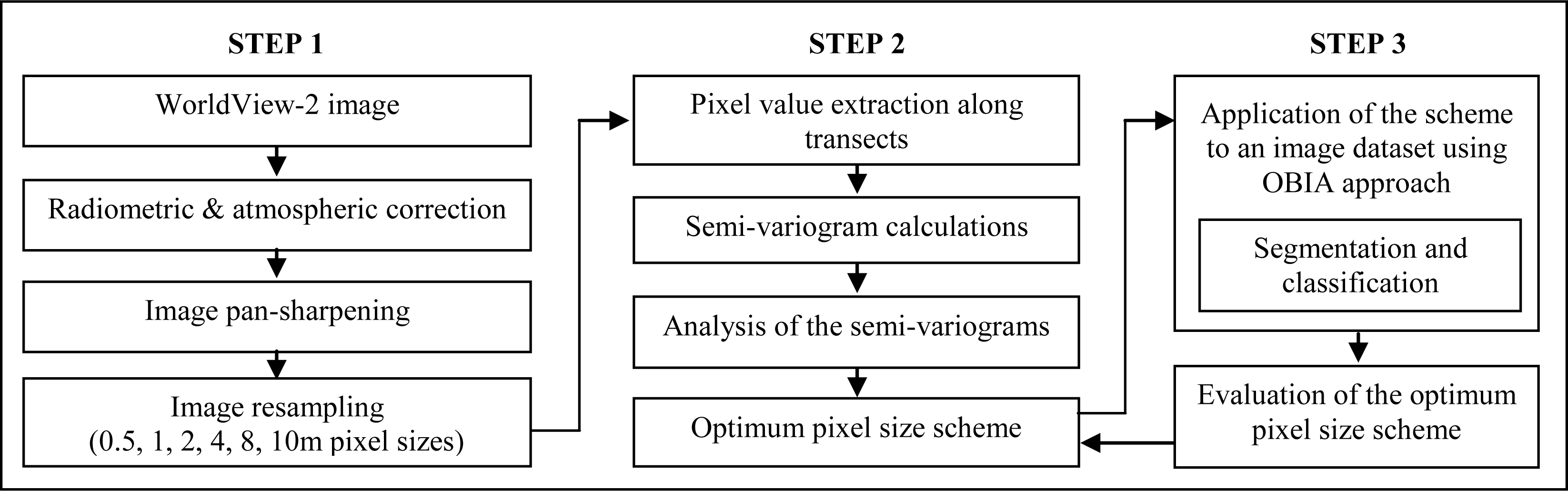
The image data used as a basis for mangrove spatial structure examination was a WorldView-2 image of the Brisbane River mouth captured on 14 April 2011 (Figure 1 and Table 1). The image was obtained in an ortho-rectified format, corrected at Level 3X (LV3X); with root-mean-square error (RMSE) 2D of 0.00 [36]. Radiometric correction was applied to the image to convert the pixel values from digital number to top-of-atmosphere spectral radiance (W/cm2sr.nm) using the values provided by Updike and Comp [37]. The atmospheric correction converting top-of-atmosphere spectral radiance to at surface reflectance was performed using the Fast Line-of-sight Atmospheric Analysis of Hypercubes (FLAASH) Atmospheric Correction Model in Environment for Visualizing Images (ENVI) 4.8, with the atmospheric visibility parameter estimated from the moderate-resolution imaging spectroradiometer (MODIS) aerosol product [38]. A very high-spatial resolution aerial photograph (Table 1) captured on 14 January 2011 ( www.nearmap.com) was used to measure the dimension (i.e., spatial size) of mangrove features investigated (foliage clumping, canopy gaps, tree crown, vegetation formation or community, and vegetation cover type) and as a reference to analyze the image spatial structure.
The fieldwork was conducted during April 2012, to measure selected mangrove vegetation structure and composition variables in the study area. Fifteen representative 200 to 300 m long field transects were established perpendicular to the shoreline (Figure 1a,b). On each transect, plots of 10 m × 10 m quadrats were sampled along the transect lines as a frame to record mangrove zonation pattern and measure mangrove biophysical properties in the field, including transect and plot positions, vegetation structural information (canopy height and vegetation formation type), dominant species, and field photos.
Positions of each sampling plot (at the start and the end of the plot) were measured using Garmin eTrex Legend H hand-held GPS, using an average reading time for each point between 400 and 600 s (with the positional accuracy of 4–6 m) to maximize the GPS signal inside the mangrove canopy. Additional control points identifiable from the field and image were used to ensure the precise overlay of the transects to the image. Canopy height was measured every 5 m along the transect using a TruPulse 360 laser rangefinder. The mangrove structural formation on each plot was determined using Australian vegetation structural formations table [35] and the dominant species information were identified using Australian mangrove identification wheel [34]. The structural characteristics measured along the transect in each of three mangrove field sample sites are presented in Table 2.

2.3. Methods

Figure 2 summarizes the methods used to measure the spatial structure of mangrove features in the study area. The work flow is divided into three steps. Step 1 is necessary to prepare the data and create a series of images with different pixel sizes as a basis for multi-scale level examination of mangrove spatial structure. Step 2 deals with measuring and analyzing the spatial structure of mangrove vegetation from the pre-processed images using semi-variograms. Step 3 applies and evaluates the results from step 2 into image datasets for mapping mangrove features using object-based image analysis (OBIA).

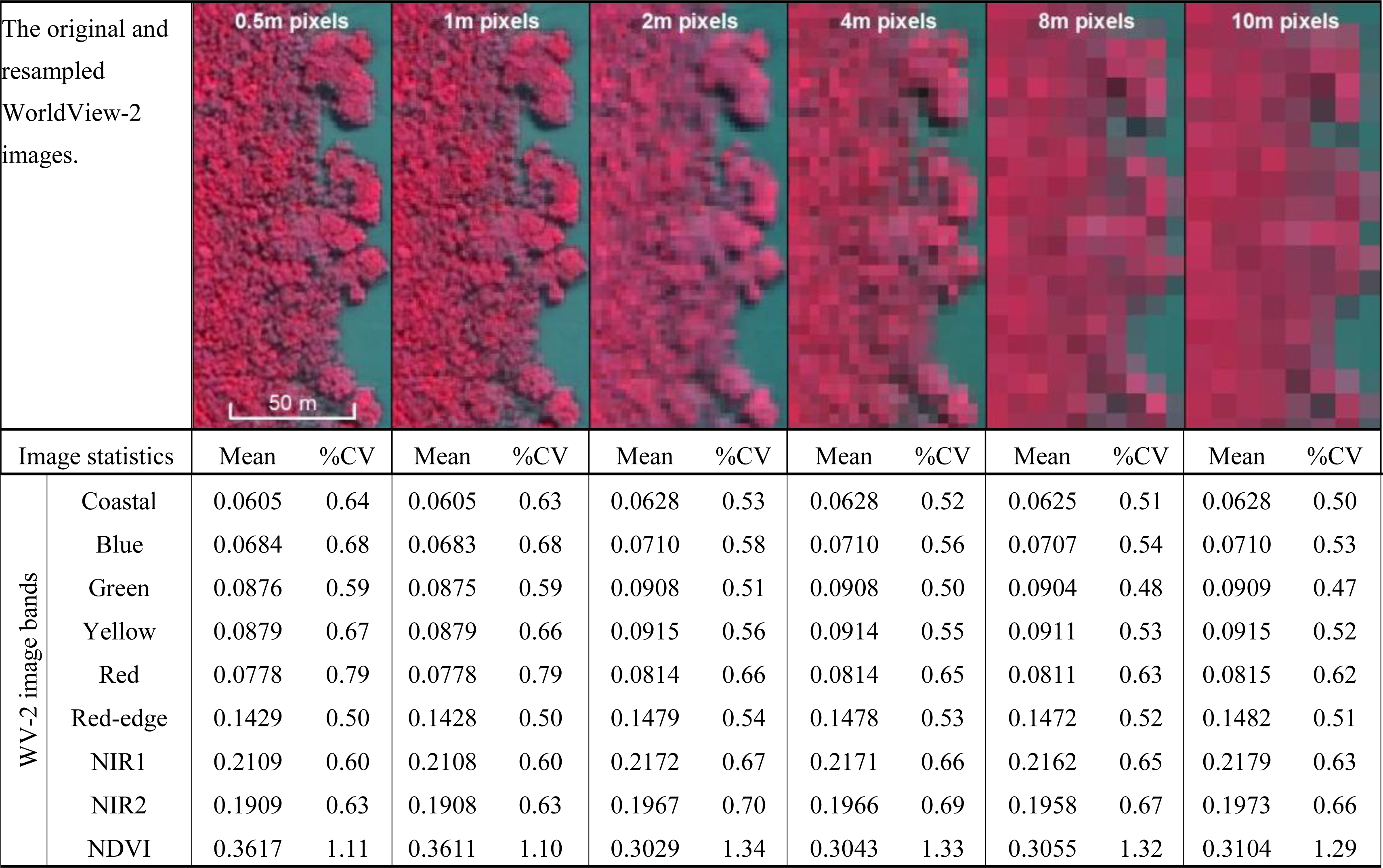
2.3.1. Image Dataset Preparation

Pan-sharpening algorithms were applied to the atmospherically corrected images to obtain a higher spatial resolution image for input to the spatial structure analysis. Six different pan-sharpening algorithms (principal component, multiplicative, Brovey, wavelet, Gram-Schmidt, and color normalized) from commercial image processing software were investigated to determine their quality in terms of preserving pixel values of the atmospherically corrected multi-spectral data. Several image quality metrics were applied, including root mean square error, standard deviation, relative shift of the mean, and coefficient of correlation [39,40]. The overall evaluation of the image quality metrics shows that the Gram-Schmidt pan-sharpening algorithm produced the pixel values closest to the original multi-spectral data, and therefore this method was used to produce a sharpened image for spatial structure analysis.
To enable analysis of the spatial structure of mangroves at multiple specific-scales and to examine the effect of different pixel sizes on the derived information, the Gram-Schmidt pan-sharpened images (0.5 m pixels) were resampled to a pixel size of 1 m, and the original multi-spectral image (2 m pixels) were resampled to 4, 8, and 10 m pixel sizes using an averaging algorithm. According to Bian and Butler [41], the pixel aggregation method is more appropriate for processing remote sensing images because a pixel value is assumed to be the averaged value over the associated area on the ground. This process produced a total of six different image pixel sizes (0.5, 1, 2, 4, 8, and 10 m). The reasons for selecting these pixel sizes were to detect specific details of mangrove features, and an approximation of the currently available image datasets. All of processing above was done using ENVI 4.8 image processing software.

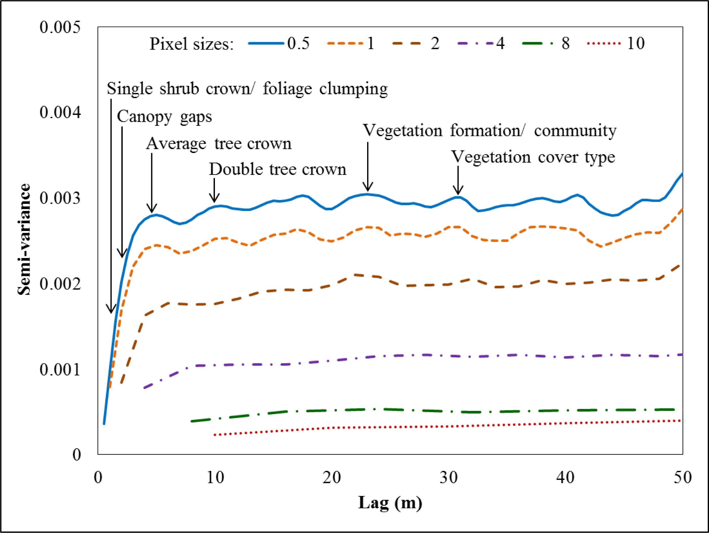
2.3.2. Measurement of Mangrove Spatial Structure through Semi-Variogram

The semi-variogram (γ) is a spatial statistical graph of semi-variance, which is the measured difference in variance value between pairs of regionalized variable samples in relation to their spatial separation with a given relative orientation. It provides a concise and unbiased description of the scale(s) and pattern(s) of spatial variability, in both remotely-sensed data and field data [42,43]. If applied to remotely-sensed data; the semi-variogram is used to examine the relation between the digital number (DN) or pixel value of n pixel pairs at a distance h (the lag distance) apart. The equation for semi-variance γ(h) is:
γ ( h ) = 1 2 n { D N ( x ) D N ( x + h ) } 2
where γ(h) represents half of the mathematical expectation of the squared differences of pixel pair values at a distance, h, and DN refers to spectral reflectance or vegetation index in this study. Hence, for image spectral data, γ(h) estimates the variability of DNs, as a function of spatial separation.
In creating semi-variograms, the distance of each lag determines the number of the pixel pairs in the transect sample. By increasing the lag distance, the pixel pairs on a transect are fewer; which in turn decreases the confidence level of the analysis [42]. To alleviate this problem, Webster [44] suggested to use lag distances shorter than a fifth of the transect length for the semi-variogram interpretation. The analysis of semi-variograms requires two assumptions: spatial stationarity, which assumes that the correlation between variables is a function of the lag distance between pixels, not because of the variation in spatial position of the transect [21,27,45]; and ergodicity, which assumes that spatial statistics taken over the area of the image as a whole are unbiased estimates of those parameters [46]. Both of these assumptions are appropriate in digital remotely-sensed images; first, because of the variation in scan angle and terrain effects are minimal and, hence, regarded as stationary in increments, and second, the reflectance surface is considered stochastic [46]. However, according to Curran [42], all image bands and directions should be examined in order to define the minimum range of the semi-variogram and therefore the minimum spatial resolution of the feature element. There are two sampling methods used in creating semi-variograms [29,47]; (1) transect method, where the semi-variogram is calculated along a single, representative row or column of pixels from each selected image, and (2) matrix method, where the semi-variogram is calculated for all the row and column pixels in each image. For canopy structure analysis, the transect sampling method provides more detailed sill variation and periodicity, and also smaller range distance compare to the matrix method [29]. It was as a result of averaging the semi-variograms for all row and column directions in matrix method. Therefore, the first sampling method was adopted for this study in order to depict structural information inherent within each of the mangrove zones.
The approach used for examining spatial structure in this study was similar to the one conducted by Cohen et al. [29], and Johansen and Phinn [24]. We used several transects created over the image data sets (original and resampled WorldView-2 images) to generate semi-variograms. All eight bands of the WorldView-2 image (Table 1), and the derived normalized difference vegetation index (NDVI) images were used to generate the semi-variograms. According to image visual inspection and semi-variogram evaluation [48], four bands (green, red-edge, near infrared1 (NIR1), NDVI) were sensitive to mangrove vegetation variations and had the least redundant information among other bands. Therefore only these bands were used for further analysis of the semi-variograms. The semi-variogram transects were located parallel to the coastline to represent the homogenous areas within each mangrove zone (i.e., areas assumed to have similar vegetation structural properties). In this study, 12 representative transects located parallel to the coastline at a distance of 25 m, 75 m, 125 m, and 175 m from the coastline were used to develop semi-variograms within zone structures (Figure 1c). The distance of the transects line varied between 500 and 1,000 m, depending on the length of the mangrove zonation. All transects were evaluated at six different pixel sizes (0.5, 1, 2, 4, 8, and 10 m). We used Earth Resources Data Analysis System (ERDAS IMAGINE) 2013 to extract pixel values along the semi-variogram transects and GS+ geostatistical software for semi-variance calculation.

2.3.3. Interpretation of Semi-Variograms

In order to interpret a semi-variogram, it is necessary to understand the term and characteristics associated to the semi-variogram (Figure 3). The range (a) of semi-variograms is a distance at which samples become independent, and it is controlled by the size of dominant objects in an image. The height of the sill (s), where the semi-variogram levels off, is considered proportional to the density of objects and scene-scale level of variance. The form of semi-variograms is controlled by the pattern and distribution of objects in an image [18,19,45,49]. These descriptors of semi-variograms are usually used together to interpret the appropriate spatial resolution for mangrove elements.
The advantage of using semi-variograms in remote sensing is its ability to relate its descriptors to the spatial characteristics of the scene [50]. The range and sill were extracted from all semi-variograms of transects located parallel and perpendicular to the coastline using the green, red-edge, NIR1, and NDVI bands. Six different image pixel sizes were evaluated to detect the scale at which certain features within each mangrove zone occurred. The range provides a measure of the size of the elements or features in the mangrove environment in the image and has been suggested as a useful indicator for selecting the optimal spatial resolution for discriminating features embedded in the semi-variogram [19,42]. Visual inspection of the field data and visual interpretation of the image were conducted in order to relate the semi-variogram range values to the mangrove vegetation structure dimensions (foliage clumping, canopy gap and tree crown size, vegetation formation, or community and vegetation cover type). This information provides guidance for developing a scheme in selecting the optimum image spatial resolution to extract specific mangrove feature, and serve as a basis for an inversion mapping approach. A total of over 1,500 semi-variograms were analyzed in this study. The findings from the semi-variogram analysis revealed the spatial characteristics of mangrove vegetation features and the optimum pixel sizes to map these features.

2.3.4. Application of the Analysis Results

To test the applicability and validate the results, we used object-based image analysis (OBIA) applied to the original and resampled WorldView-2 images with the segmentation and classification being driven by parameters obtained from the semi-variogram analysis. OBIA offers some fundamental advantages in the context of this study, including: (1) image objects can be created at multiple, yet specific, hierarchical spatial scales (e.g., tree community consists of several single tree canopies) [51,52], (2) numerous attributes can be obtained from image objects, such as object’s statistics, geometry and context, (3) better mimics human perception of real-world objects [53], and (4) image objects reduce the salt-and-pepper effect in pixel-based classifications [54].
We applied image segmentation and classification to the original and resampled WorldView-2 images to evaluate the applicability of the semi-variogram results. The segmentation and classification routines were carried out using eCognition Developer software v. 8.7.0. A series of scale parameters from 5 to 100 were tested for the mapping of mangrove features with a weight of 5 applied to the green, red, red-edge, and NIR1 bands to enhance the influence of bands that are sensitive to vegetation reflectance in the segmentation. We used a trial-and-error approach and visual inspection of the segmentation results with the help of a very-high-spatial resolution aerial photograph (7.5 cm pixel size) to determine the mangrove features that can be depicted from different scale parameters and image pixel sizes.
A supervised rule-based classification was applied to implement the optimum pixel size scheme for mangrove feature mapping based on the WorldView-2 images. The rule sets were developed using the objects’ spectral information, geometry of the objects, and contextual hierarchy of the classes. The first hierarchy layer was used to separate mangrove and non-mangrove features, the second layer was for dividing the mangrove area into trees and gaps (and shadows), and the third layer, was used for classification of objects within the mangrove tree class. These hierarchical layers were applied to all image pixel sizes being examined. The result of the mapping was used to evaluate the image selection scheme and inversion mapping approach.

3. Results and Discussion

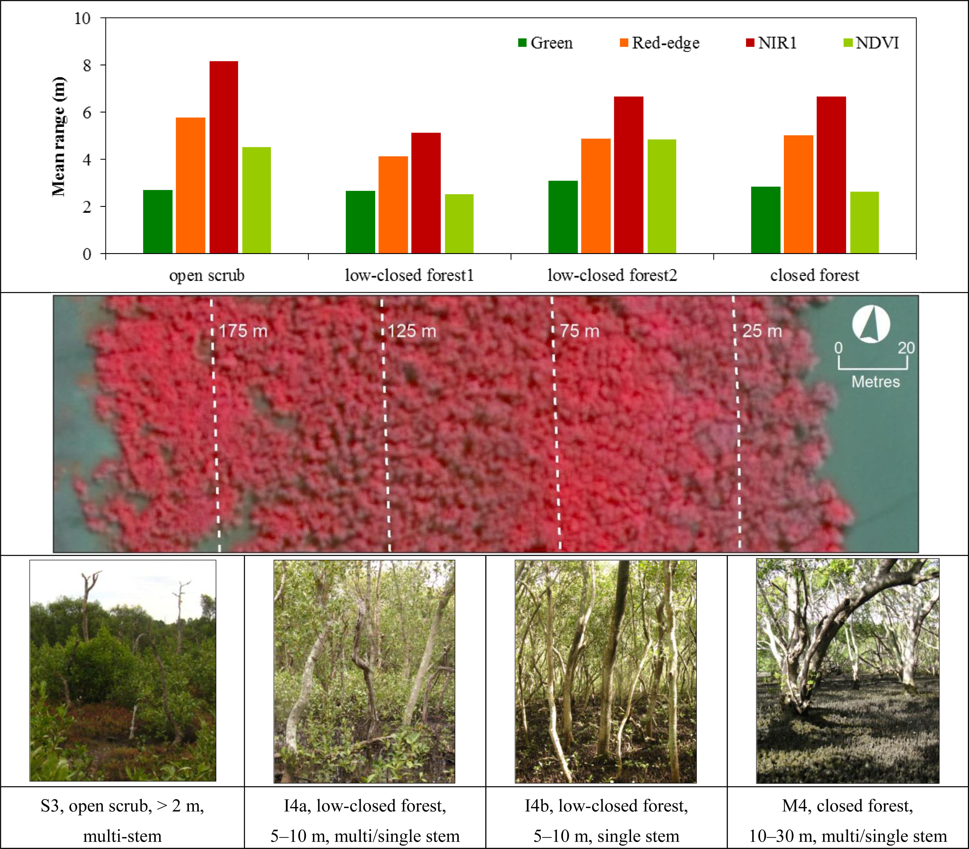
3.1. Relation of Semi-Variograms to Mangrove Vegetation Structure Properties

Visual characteristics of the images demonstrate the gradual loss of mangrove spatial structure detail by the increasing pixel sizes (Figure 4). The descriptive statistics for each image shows the divergence between original (0.5 and 2 m) and resampled image (1, 4, 8, and 10 m). While the mean values of the bands in the resampled image exhibit some random variations, the coefficient of variance (%CV) decreased with decreasing spatial resolution relative to the original images. The coastal and yellow bands for the first resampling group (from 0.5 to 1 m) and all bands for the second resampling group (from 2 to 10 m) also follow this pattern. Figure 4 shows that an image with lower spatial resolution has lower data variability and therefore contains less information compared to a higher spatial resolution image.
The spatial structural information of mangrove elements (or features) detectable from the original and resampled WorldView-2 images was related to the semi-variogram descriptors (range, sill, and form). Figure 5 (preliminary published in [48]) shows the representative semi-variogram plot of the near infrared1 (NIR1) image band at six different pixel sizes, and the average mangrove feature sizes measured from field-work and the aerial photograph. It reveals similar results to those presented in other studies examining the effects of changes in image pixel size on image information content [19,24,29,55,56]. Specifically, there is a gradual loss of information detail with the increasing pixel size (Figure 4 and 5). The forms of semi-variogram changes with the varying pixel sizes describe the effect of data regularization on the spatial heterogeneity component. The decreasing height of the sill characterizes the loss of spatial variability when the spatial resolution of the image decreases, which is also evident in the image statistics in Figure 4.
At a pixel size of 0.5 m, the form of semi-variograms appears to be controlled by inter-canopy features including individual shrubs and tree crown, foliage clumping and smaller inter-canopy gaps. At a pixel size of 1 m, the individual shrub and tree crown are still distinguishable, but the detailed foliage clumping and inter-canopy gaps become more difficult to identify. Single shrub crowns and foliage clumping identified from the image and field data correspond to the semi-variogram lag distance of 1.5 m, and the inter-canopy gaps at 2 m. Pixel sizes 0.5 and 1 m had similar semi-variogram forms, meaning the variation of information of the pattern and distribution of mangrove features within these sizes are comparable, but they have different sill height which is attributed to the different level of pixel value variance in the image scene (see image statistics in Figure 4). Although these two pixel sizes offer similar capability, detailed information on structural properties and sharper visual image appearance increases the likelihood of correctly identifying mangrove inter-canopy features.
The range of the semi-variograms for pixel sizes 2 m and smaller are all at 5 m, which is approximately equal to the average diameter of single mangrove tree crowns. This indicates that single mangrove tree crowns may be distinguished at a maximum pixel size of 2 m. At a pixel size of 4 m the average single tree crown is no longer apparent, although some individual larger canopies of mangrove tree and gaps that are more than 10 m in diameter can still be identified. Based on field observations, it is likely that the range of about 8 to 10 m corresponds to groups of two tree crowns, and these can be identified at pixel sizes of 4 m. The semi-variogram range of pixel sizes of 8 and 10 m are approximately 20 and 30 m, respectively, which correspond to the average size of mangrove vegetation formation or community at 23 m and larger mangrove cover types at 30 m. At a pixel size of 4 m and larger, the canopy-related information is gradually lost. They are more appropriate for mapping larger mangrove communities, mangrove patches, and separating mangroves from non-mangrove cover types.
Overall, there are noticeable patterns of semi-variogram peaks and troughs with different sill heights across varying pixel sizes. According to Figure 5, the variation of structural information within mangrove stands can only be preserved by pixel sizes of 0.5 to 2 m, where the semi-variogram contains periodic peaks and troughs along the graph. On the other hand, from pixel sizes of 4 to 10 m, these variations are lost and result in relatively flat graphs with minimum or no information on within mangrove structural properties. This finding indicates that pixel sizes of 2 m and smaller are appropriate for mapping small size features and internal variation of mangrove canopy (such as single shrub crown, foliage clumping, canopy gaps, and average tree crown), whereas pixel sizes of 4 m and larger are more appropriate to map larger mangrove features (such as groups of tree crowns, vegetation formations or communities, and cover type).

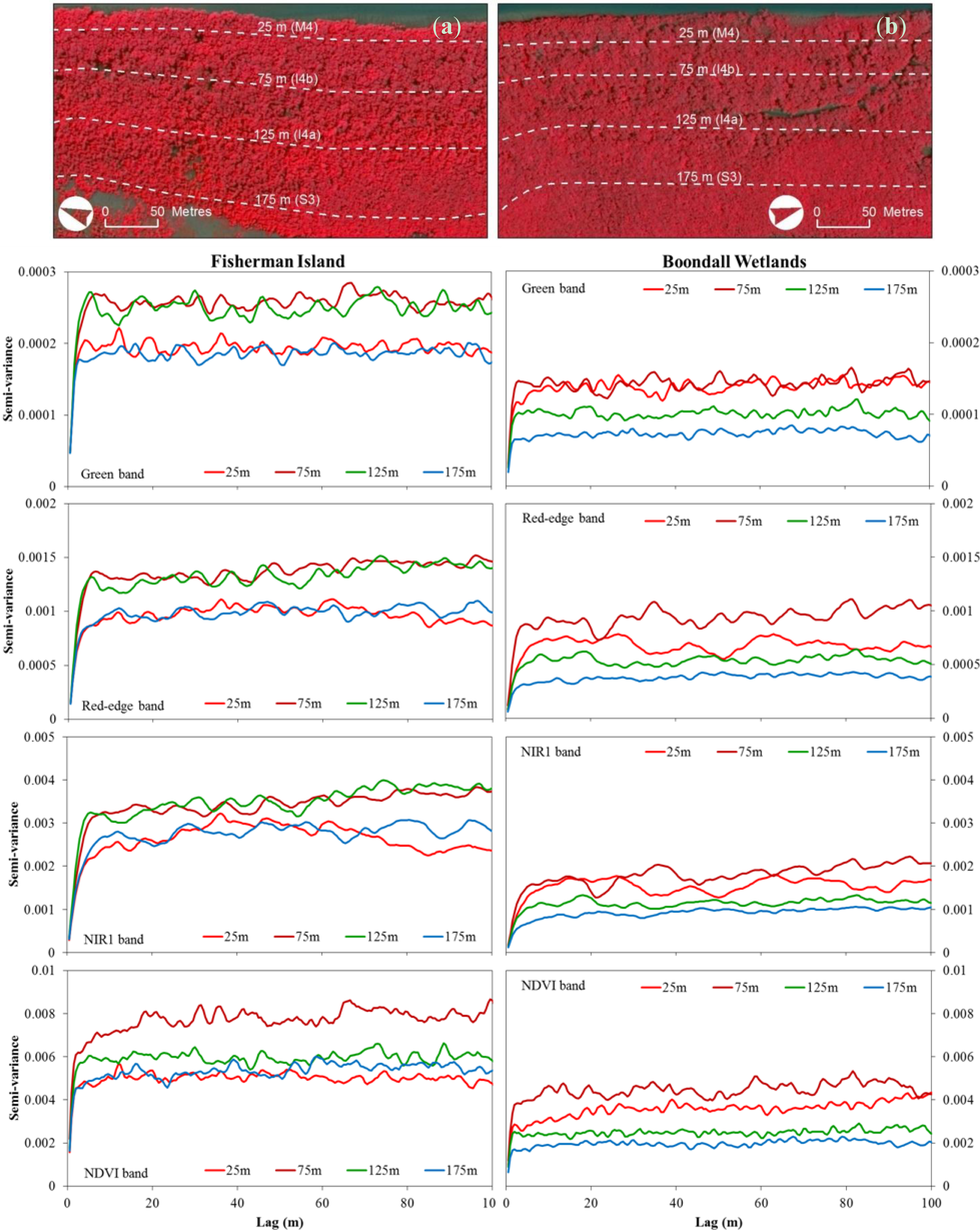
3.2. Relation of Semi-Variograms to Mangrove Zone Features

Variation in spatial structural information between mangrove zones, i.e., areas with consistent structure and composition parallel to the coastline, were examined using transects located parallel to the coastline at varying distances from the three Moreton Bay sites. The semi-variograms were derived from transects of 1000 m in length along the mangrove zonation which were located at distances of 25, 75, 125, and 175 m from the edge of outer mangrove stands. These distances were selected to be as representative as possible of mangrove zonation to depict the within mangrove zonation structural properties. Among the three transect locations; two of them produced similar semi-variograms. Therefore, only two of the transect locations are discussed here, which are Fisherman Island and Boondall wetlands (Figure 6).
The transect at 125 m from the coastline on Fisherman Island had high sill values and was the second highest for all of the bands. It corresponds to a low-closed forest mangrove formation where there are mixed stems of Avicennia marina trees (I4a) with high canopy cover and some canopy gaps. For the Boondall wetlands, this transect distance was at the third highest level of the semivariogram sill height. The mixed-stem low-closed forest (I4a) formation in Boondall has a lower canopy cover and more canopy gaps, making it appear to have low contrast in the image. Finally, transects located at a distance of 175 m from the coastline had the lowest semi-variogram sill values and this pattern is noticeable for all bands and all locations. These transects cover the open scrub Avicennia marina zone with low density of canopy cover and uniform canopy layers. Some gaps with Sarcocornia quinqueflora, water or soil are also frequently found in this zone, which may contribute to decreasing the reflectance intensity of the pixels.
Semi-variograms located along the mangrove zones revealed different spatial structural characteristics of mangrove features within each zonation. As shown in Figure 7, the average range of semi-variograms of all evaluated bands for transects located along the mangrove zonation at the Moreton Bay sites exhibit different patterns. The average range values of open scrub formation (S3) were higher for all of the image bands (2.7 to 8.1 m) compared to the other formations, where low-closed forest1 (I4a) had the lowest average range value (2.5 to 5.2 m), and low-closed forest2 (I4b) together with closed forest (M4) had a similar range value (3.1 to 6.6 and 2.6 to 6.6 m, respectively). The high average range values on the open scrub formation (S3) were attributed to the large variation in the size of Avicennia marina scrub patches interleaved with large gaps of ground or water that are frequently found in this zone (see image on Figure 7). Conversely, the low average range values of the low-closed forest1 (I4a) were caused by the foliage clumping and the narrow canopy gaps (1–2 m) between individual tree crowns (approximately 5 m in diameter) that dominate this zone.

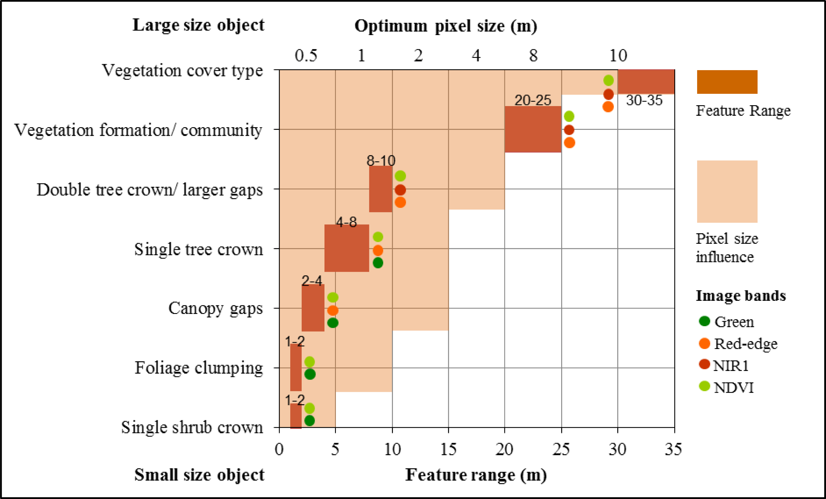
3.3. Optimum Pixel Size for Mangrove Mapping

Several transects were established along the mangrove zonation at the Moreton Bay sites to create semi-variograms to depict the variation of spatial size of the structural features of mangroves. The information on the characteristics of spatial structure of mangrove features obtained from semi-variogram interpretation and analysis provides the basis for establishing the relationship between mangrove feature sizes and optimum spatial resolution (i.e., image pixel size) to map these features. According to techniques used in the previous semi-variogram analyses, seven mangrove vegetation structures were apparent in the study area and detectable from the WorldView-2 image data. These included single shrub crown, small foliage clumping within canopy or intra-canopy, smaller canopy gaps, average single tree crown, double tree crown or larger gaps, vegetation structural formation/community, and vegetation cover type. By integrating semi-variogram interpretation results at specific pixel sizes along mangrove zonations, with field data and image interpretation, it was apparent that each of these mangrove features resided within certain range distances and can only be detected at specific image pixel sizes.
Figure 8 illustrates the relationships between the range of mangrove features, the optimum pixel size, and the most appropriate spectral bands able to identify and map these features. The mangrove structural features were plotted on the y axis from the largest scale at the bottom to the smallest scale at the top of the axis. Seven plot boxes inside the graph depict where the mangrove features on the y axis reside along the feature range distance (bottom x axis); and the downward bar charts from the x axis at the top illustrate the influence of the associated pixel size on the plot boxes of mangrove features. The most appropriate spectral bands were placed as dot point indicators beside the associated mangrove feature. For example, the average single tree crown has semi-variogram range values between 4 and 8 m. This feature can be identified using image pixel sizes of 0.5, 1, and 2 m, but is unable to be identified at a pixel size of 4 m or larger. Therefore, in this case, an image with a pixel size of 2 m is the optimum option to map the average mangrove tree crown as it is the largest pixel size able to identify individual tree crowns, and green, red-edge, and NDVI bands will be the most suitable bands for discriminating this feature. For mapping routine purposes, using an image datasets with a smaller pixel size will increase the cost, both for resources and processing, and may produce the result that is similar to a product derived from the optimum pixel size.

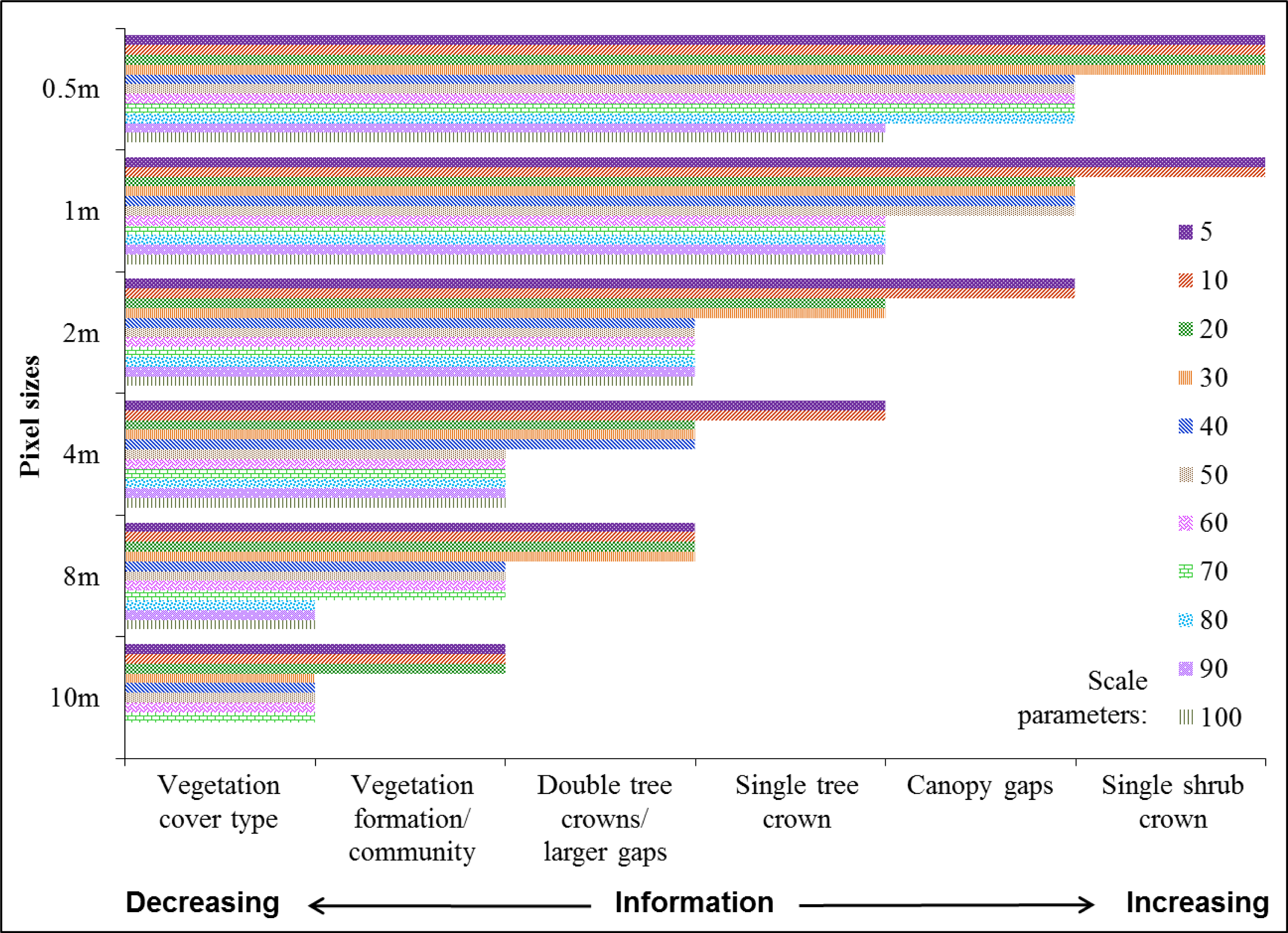
3.4. Application of the Optimum Pixel Size Scheme

The pattern of mangrove feature information obtained from different scale parameters applied to different image pixel sizes was interpreted from the image segmentation results (Figure 9). In accordance to the results of the semi-variogram analysis; the lower value of the scale parameter or the smaller pixel size, the more mangrove information could be extracted from the image. According to the interpretation results, single shrub crowns could only be recognised at a pixel size of 0.5 m with the segmentation scale parameter ≤30, and at a pixel size of 1 m with the scale parameter ≤10. At a pixel size of 2 m, the smallest obtainable mangrove objects were canopy gaps and single tree crowns with a segmentation scale parameter ≤10 and 20–30, respectively. At a scale parameter ≥40 the segment size was too large and failed to identify single tree crowns. Most of the pixel sizes ≥2 m could only differentiate objects larger than the average size of single tree crowns, including double/multiple tree crowns, larger gaps, vegetation formation and community, and vegetation cover types; with the exception of scale parameters ≤10 at a pixel size 4 m, which still allowed discrimination of single tree crowns. In general, there was an obvious relationship between mangrove information detail and the pixel and segmentation scale parameter size, where smaller pixel sizes or segmentation scale parameters will allow more detailed mapping of mangrove features.
We also identified the size of dominant objects able to be delineated in the segmentation process from six different pixel sizes and related the result with the measured feature dimension in the field. The dominant segment sizes and the corresponding pixel sizes were found to correspond well to the result of the optimum pixel sizes from the semi-variogram analysis (Columns c and f in Table 3). The result indicated that the theoretical finding of the optimum pixel sizes from the SV is empirically proven on the image dataset through image segmentation.
The classification results showed that the use of each image pixel size enabled the discrimination of the smallest mangrove object according to the previously developed optimum pixel size scheme (Figure 8). Figure 10 shows some selected examples of the classification results applied to the image at pixel sizes of 0.5, 2, and 8 m to depict information of shrub crown, single tree crown, and mangrove formation, respectively. We used a very-high-spatial resolution aerial photograph as a reference to assess and evaluate the quality of mangrove feature mapping. This was used as there was no existing map containing mangrove vegetation features for the study area, and the aerial photograph interpretation was accepted to be correct (due to the features evident at very high resolution) without any form of accuracy assessment [57].
At a pixel size of 0.5 m individual shrub crowns were discriminated from other features, but the classification was unable to identify each single shrub crown in groups of shrub (Figure 10a) due to the short distance between the crowns and the shape similarity. Single stands of tree crowns were well identified at pixel size of 2 m, although the segments were blocky due to the bigger pixel size (Figure 10b). Individual trees in the mangrove forest were difficult to distinguish because of their closed canopy and similarity to the neighbouring objects (i.e., tree crowns). Four mangrove formations found in the study area were clearly separated at a pixel size of 8 m (Figure 10c), with some isolated segments found within the formation. According to the qualitative segmentation assessment, the optimum pixel size scheme worked well when applied to the image datasets used in this study. As the segmentation and classification example was purely used as a proof of concept, further improvements to the segmentation and classification process are still possible to improve the mapping accuracy and repeatability across other areas.

4. Conclusions and Future Research

This study showed that scale-specific, ecologically relevant information on mangroves can be detected using experimental semi-variogram analysis. This approach indicated the size of dominant mangrove features able to be identified from a specific pixel size and the optimum spectral bands to use to detect and map these features. The results show that there was a gradual loss in mangrove vegetation structural information, as indicated by mangrove features measured, with increasing pixel size. When applied to the original and resampled WorldView-2 images, we found that a pixel size ≤2 m was suitable for mapping canopy and inter-canopy related features within mangrove objects (such as shrub crown, canopy gaps, single tree crown). A pixel size of ≥4 m was more appropriate for mapping mangrove vegetation formation, communities and larger mangrove features. The green and red-edge bands were optimum for discriminating smaller sized mangrove features (<8 m), such as single shrub crown or foliage clumping, canopy gaps, and single tree crown. The near infrared1 band was more suitable for identifying feature ≥8 m (e.g., double tree crown or larger gaps), and the NDVI image was suitable for mapping all targeted features.
The findings of this study provide a basis for an inversion approach to mangrove feature mapping using high-spatial resolution image datasets. The mapping application results demonstrated that the optimum pixel size scheme from the semi-variogram analysis was effectively applied through image segmentation and classification using object-based image analysis. The optimum pixel analysis result from the image segmentation interpretation was highly correlated with the semi-variogram results, and the classification result identified the smallest features that could be discriminated at the corresponding pixel size.
The results of this work were limited to the study site in Moreton Bay, Australia, with sub-tropical mangroves. For future research, the application of the experimental semi-variogram method to other mangrove environments is necessary to assess the consistency of the method. In terms of the mapping application, further development of object-based classification rule sets is essential for improving the detection of multi-scale mangrove features and determining the transferability and general applicability of the findings.

Acknowledgments

This study is a component of Kamal’s PhD project on multi-scale image-based mangrove mapping undertaken at The University of Queensland. The authors would like to thank Digital Globe for providing the WorldView-2 images; Biophysical Remote Sensing Group (BRG) at The University of Queensland (UQ) for providing research facilities and publication funding; School of Geography, Planning and Environmental Management (GPEM) UQ for research funding and fieldwork support; Ralph Dowling and Arnon Accad from Queensland Herbarium for mangrove mapping and fieldwork discussion; and Novi Adi (BRG UQ) for assistance with fieldwork. Authors would also like to thank the anonymous reviewers whose comments were detailed and constructive, improving the overall quality of the paper.

Author Contributions

Muhammad Kamal performed the image processing and analysis and prepared the manuscript, Stuart Phinn and Kasper Johansen contributed to the design of the work, discussion and edited drafts.

Conflicts of Interest

The authors declare no conflict of interest.

References

  1. Davis, B.A.; Jensen, J.R. Remote sensing of mangrove biophysical characteristics. Geocarto Int 1998, 13, 55–64. [Google Scholar]
  2. Ramsey, E.W., III; Jensen, J.R. Remote sensing of mangrove wetlands: Relating canopy spectra to site-specific data. Photogramm. Eng. Remote Sens 1996, 62, 939–948. [Google Scholar]
  3. Kuenzer, C.; Bluemel, A.; Gebhardt, S.; Quoc, T.V.; Dech, S. Remote sensing of mangrove ecosystems: A review. Remote Sens 2011, 3, 878–928. [Google Scholar]
  4. Malthus, T.J.; Mumby, P.J. Remote sensing of the coastal zone: An overview and priorities for future research. Int. J. Remote Sens 2003, 24, 2805–2815. [Google Scholar]
  5. Heumann, B.W. Satellite remote sensing of mangrove forests: Recent advances and future opportunities. Prog. Phys. Geogr 2011, 35, 87–108. [Google Scholar]
  6. Wiens, J.A. Spatial scaling in ecology. Funct. Ecol 1989, 3, 385–397. [Google Scholar]
  7. Delcourt, H.R.; Delcourt, P.A.; Webb, T., III. Dynamic plant ecology: The spectrum of vegetational change in space and time. Quat. Sci. Rev 1983, 1, 153–175. [Google Scholar]
  8. Schaeffer-Novelli, Y.; Cintrón-Molero, G.; Cunha-Lignon, M.; Coelho, C., Jr. A conceptual hierarchical framework for marine coastal management and conservation: A “Janus-like” approach. J. Coast. Res 2005, 191–197. [Google Scholar]
  9. Feller, I.C.; Lovelock, C.E.; Berger, U.; McKee, K.L.; Joye, S.B.; Ball, M.C. Biocomplexity in mangrove ecosystems. Annu. Rev. Mar. Sci 2010, 2, 395–417. [Google Scholar]
  10. Farnsworth, E.J. Issues of spatial, taxonomic and temporal scale in delineating links between mangrove diversity and ecosystem function. Glob. Ecol. Biogeogr. Lett 1998, 7, 15–25. [Google Scholar]
  11. Lee, D.; Grant, W. A hierarchical approach to fisheries planning and modeling in the Columbia River Basin. Environ. Manag 1995, 19, 17–25. [Google Scholar]
  12. Müller, F. Hierarchical approaches to ecosystem theory. Ecol. Model 1992, 63, 215–242. [Google Scholar]
  13. Woodcock, C.E.; Strahler, A.H. The factor of scale in remote sensing. Remote Sens. Environ 1987, 21, 311–332. [Google Scholar]
  14. Phinn, S.R.; Menges, C.; Hill, G.J.E.; Stanford, M. Optimizing remotely sensed solutions for monitoring, modeling, and managing coastal environments. Remote Sens. Environ 2000, 73, 117–132. [Google Scholar]
  15. Goodchild, M.F.; Quattrochi, D.A. Scale, Multiscaling, Remote Sensing, GIS. In Scale in Remote Sensing and GIS; Quattrochi, D.A., Goodchild, M.F., Eds.; CRS Press: Boca Raton, FL, USA, 1997; pp. 1–12. [Google Scholar]
  16. Marceau, D.J.; Hay, G.J. Remote sensing contributions to the scale issue. Can. J. Remote Sens 1999, 25, 357–366. [Google Scholar]
  17. Raffy, M. Change of scale theory: A capital challenge for space observation of earth. Int. J. Remote Sens 1994, 15, 2353–2357. [Google Scholar]
  18. Woodcock, C.E.; Strahler, A.H.; Jupp, D.L.B. The use of variograms in remote sensing: I. Scene models and simulated images. Remote Sens. Environ 1988, 25, 323–348. [Google Scholar]
  19. Woodcock, C.E.; Strahler, A.H.; Jupp, D.L.B. The use of variograms in remote sensing: II. Real digital images. Remote Sens. Environ 1988, 25, 349–379. [Google Scholar]
  20. Colombo, S.; Chica-Olmo, M.; Abarca, F.; Eva, H. Variographic analysis of tropical forest cover from multi-scale remotely sensed imagery. ISPRS J. Photogramm. Remote Sens 2004, 58, 330–341. [Google Scholar]
  21. Treitz, P.; Howarth, P. High spatial resolution remote sensing data for forest ecosystem classification: An examination of spatial scale. Remote Sens. Environ 2000, 72, 268–289. [Google Scholar]
  22. Hyppanen, H. Spatial autocorrelation and optimal spatial resolution of optical remote sensing data in boreal forest environment. Int. J. Remote Sens 1996, 17, 3441–3452. [Google Scholar]
  23. Wolter, P.T.; Townsend, P.A.; Sturtevant, B.R. Estimation of forest structural parameters using 5 and 10 meter SPOT-5 satellite data. Remote Sens. Environ 2009, 113, 2019–2036. [Google Scholar]
  24. Johansen, K.; Phinn, S. Linking riparian vegetation spatial structure in Australian tropical savannas to ecosystem health indicators: Semi-variogram analysis of high spatial resolution satellite imagery. Can. J. Remote Sens 2006, 32, 228–243. [Google Scholar]
  25. Menges, C.H.; Hill, G.J.E.; Ahmad, W. Use of airborne video data for the characterization of tropical savannas in northern Australia: The optimal spatial resolution for remote sensing applications. Int. J. Remote Sens 2001, 22, 727–740. [Google Scholar]
  26. He, Y.; Guo, X.; Wilmshurst, J.; Si, B.C. Studying mixed grassland ecosystems II: Optimum pixel size. Can. J. Remote Sens 2006, 32, 108–115. [Google Scholar]
  27. Phinn, S.; Franklin, J.; Hope, A.; Stow, D.; Huenneke, L. Biomass distribution mapping using airborne digital video imagery and spatial statistics in a semi-arid environment. J. Environ. Manag 1996, 47, 139–164. [Google Scholar]
  28. Wen, Z.; Zhang, C.; Zhang, S.; Ding, C.; Liu, C.; Pan, X.; Li, H.; Sun, Y. Effects of normalized difference vegetation index and related wavebands’ characteristics on detecting spatial heterogeneity using variogram-based analysis. Chin. Geogr. Sci 2012, 22, 188–195. [Google Scholar]
  29. Cohen, W.B.; Spies, T.A.; Bradshaw, G.A. Semivariograms of digital imagery for analysis of conifer canopy structure. Remote Sens. Environ 1990, 34, 167–178. [Google Scholar]
  30. Chen, D. Multi-Resolution Image Analysis and Classification for Improving Urban Land Use/Cover Mapping Using High Resolution Imagery, San Diego State University and University of California, Santa Barbara, CA, USA, 2001.
  31. Australian Bureau of Meteorology. Available online: http://www.bom.gov.au/ (accessed on 1 February 2013).
  32. Environment Australia. A Directory of Important Wetlands in Australia, 3rd ed; Environment Australia: Canberra, ACT, Australia, 2001; p. 157. [Google Scholar]
  33. Dowling, R.M.; Stephen, K. Coastal Wetlands of South-Eastern Queensland: Maroochy Shire to New South Wales Border; Queensland Herbarium, Environmental Protection Agency: Brisbane, QLD, Australia, 2001; p. 220. [Google Scholar]
  34. Duke, N.C. Australia’s Mangroves: The Authoritative Guide to Australia’s Mangrove Plants; University of Queensland: Brisbane, QLD, Australia, 2006; p. 200. [Google Scholar]
  35. Specht, R.L.; Specht, A.; Whelan, M.B.; Hegarty, E.E. Conservation Atlas of Plant Communities in Australia; Southern Cross University Press: Lismore, NSW, Australia, 1995; p. 910. [Google Scholar]
  36. Digital Globe Digital Globe Imagery Support Data (ISD) Documentation. Available online: http://www.digitalglobe.com/sites/default/files/Imagery_Support_Data_Documentation(1).pdf (accessed on 18 December 2013).
  37. Updike, T.; Comp, C. Radiometric Use of WorldView-2 Imagery; DigitalGlobe Inc: Longmont, CO, USA, 2010. [Google Scholar]
  38. LAADS Level 1 and Atmosphere Archive and Distribution System. Website of NASA-Goddard Space Flight Center. Available online: http://ladsweb.nascom.nasa.gov/data/search.html (accessed on 5 March 2012).
  39. Jayanth, J.; Kumar, T.A.; Koliwad, S. Comparative Analysis of Image Fusion Techniques in Remote Sensing. In Advanced Machine Learning Technologies and Applications; Hassanien, A.E., Salem, A.M., Ramadan, R., Kim, T., Eds.; Springer: Berlin/Heidelberg, Germany, 2012; Volume 322, pp. 111–117. [Google Scholar]
  40. Vijayaraj, V.; O’Hara, C.G.; Younan, N.H. Quality Analysis of Pansharpened Images. Proceedings of The IEEE 2004 International Geoscience and Remote Sensing Symposium, Anchorage, AK, USA, 20–24 September 2004.
  41. Bian, L.; Butler, R. Comparing effects of aggregation methods on statistical and spatial properties of simulated spatial data. Photogramm. Eng. Remote Sens 1999, 65, 73–84. [Google Scholar]
  42. Curran, P.J. The semivariogram in remote sensing: An introduction. Remote Sens. Environ 1988, 24, 493–507. [Google Scholar]
  43. Curran, P.J.; Atkinson, P.M. Geostatistics and remote sensing. Prog. Phys. Geogr 1998, 22, 61–78. [Google Scholar]
  44. Webster, R. Quantitative spatial analysis of soil in the field. Adv. Soil Sci 1985, 3, 1–70. [Google Scholar]
  45. Bailey, T.C.; Gatrell, A.C. Interactive Spatial Data Analysis; Longman Scientific & Technical: Harlow, Essex, UK, 1995; p. 413. [Google Scholar]
  46. Jupp, D.L.B.; Strahler, A.H.; Woodcock, C.E. Autocorrelation and regularization in digital images. I. Basic theory. IEEE Trans. Geosci. Remote Sens 1988, 26, 463–473. [Google Scholar]
  47. Feng, Y.; Li, Z.; Tokola, T. Estimation of stand mean crown diameter from high-spatial-resolution imagery based on a geostatistical method. Int. J. Remote Sens 2010, 31, 363–378. [Google Scholar]
  48. Kamal, M.; Phinn, S.; Johansen, K. Assessment of Mangrove Spatial Structure Using High-Spatial Resolution Image Data. Proceedings of IEEE International Geoscience and Remote Sensing Symposium (IGARSS), Melbourne, Australia, 21–26 July 2013; pp. 2609–2612.
  49. Jupp, D.L.B.; Strahler, A.H.; Woodcock, C.E. Autocorrelation and regularization in digital images. II. Simple image models. IEEE Trans. Geosci. Remote Sens 1989, 27, 247–258. [Google Scholar]
  50. Atkinson, P.M.; Curran, P.J. Choosing an appropriate spatial resolution for remote sensing investigations. Photogramm. Eng. Remote Sens 1997, 63, 1345–1351. [Google Scholar]
  51. De Jong, S.M.; van der Meer, F.D. Remote Sensing Image Analysis: Including the Spatial Domain; Kluwer Academic Publishers: Dordrecht, The Netherlands, 2005; p. 359. [Google Scholar]
  52. Hay, G.J.; Blaschke, T.; Marceau, D.J.; Bouchard, A. A comparison of three image-object methods for the multiscale analysis of landscape structure. ISPRS J. Photogramm. Remote Sens 2003, 57, 327–345. [Google Scholar]
  53. Morgan, J.L.; Gergel, S.E.; Coops, N.C. Aerial photography: A rapidly evolving tool for ecological management. BioScience 2010, 60, 47–59. [Google Scholar]
  54. Blaschke, T.; Lang, S.; Lorup, E.; Strobl, J.; Zeil, P. Object-Oriented Image Processing in an Integrated GIS/Remote Sensing Environment and Perspectives for Environmental Applications. In Environmental Information for Planning, Politics and the Public; Cremers, A., Greve, K., Eds.; Metropolis Verlag: Marburg, Germany, 2000; 2, pp. 555–570. [Google Scholar]
  55. Chen, W.; Henebry, G.M. Change of spatial information under rescaling: A case study using multi-resolution image series. ISPRS J. Photogramm. Remote Sens 2009, 64, 592–597. [Google Scholar]
  56. Garrigues, S.; Allard, D.; Baret, F.; Weiss, M. Quantifying spatial heterogeneity at the landscape scale using variogram models. Remote Sens. Environ 2006, 103, 81–96. [Google Scholar]
  57. Congalton, R.G. A review of assessing the accuracy of classifications of remotely sensed data. Remote Sens. Environ 1991, 37, 35–46. [Google Scholar]
Figure 1. (a) Study sites: Mangroves at Moreton Bay area, Brisbane, Australia; (b) An example of field survey transect, orange circles represent location of 10 m × 10 m quadrats, and (c) Transects of image pixels running parallel to the coastline used to derive the semi-variograms shown for Whyte Island.
Remotesensing 06 00984f1
Figure 2. Overview of the methods.
Remotesensing 06 00984f2
Figure 3. An example of variogram with descriptors, and the definition of terms [24,43].
Remotesensing 06 00984f3
Figure 4. Subsets of mangrove on Whyte Island at pixel sizes of 0.5, 1, 2, 4, 8, and 10 m displayed with a band combination of R:7, G:5, B:3, and their associated descriptive statistics.Note: The mean image spectral reflectance and NDVI values were represented at a scale of 0–1, %CV: coefficient of variance
Remotesensing 06 00984f4
Figure 5. Subset of NIR1 semi-variogram showing the mangrove features responsible for the semi-variogram range and form up to a 50 m lag distance.
Remotesensing 06 00984f5
Figure 6. Subset of pan-sharpened image of (a) Fisherman Island and (b) Boondall wetlands showing the transects along the mangrove zonations, and semi-variograms created from transects along the mangrove zonation at distances of 25, 75, 125, and 175 m from the coastline using the 0.5 m pan-sharpened WorldView-2 image.
Remotesensing 06 00984f6
Figure 7. Mean semi-variogram range values sampled at 0.5 m pixel size for the green, red-edge, NIR1, and NDVI bands, based on four transects located at 175 m (S3), 125 m (I4a), 75 m (I4b), and 25 m (M4) from the coastline of Moreton Bay mangroves.
Remotesensing 06 00984f7
Figure 8. Relationship between mangrove features, feature ranges, optimum pixel sizes, and the most sensitive image bands to map mangrove features.
Remotesensing 06 00984f8
Figure 9. Graph of mangrove features detectable at a number of scale parameters derived from different WorldView-2 image pixel sizes.
Remotesensing 06 00984f9
Figure 10. Example of mangrove features segmented and classified (green polygons) from images with different image pixel sizes and scale parameters (SP).
Remotesensing 06 00984f10aRemotesensing 06 00984f10b
Table 1. Characteristics of image data used in this study.
Image TypeWorldView-2Aerial Photograph
Acquisition date14 April 201114 January 2011
Acquisition time00:10:47.59 UTC (10:10:47.59 AEST)
Product type and levelOrtho, LV3XOrtho-rectified
Geometric attributesUTM 56 J in metersGCS WGS 1984
Radiometric attributes16 bits per-pixel
Coastal (400–450 nm)
Blue (450–510 nm)
Green (510–580 nm)
Yellow (585–625 nm)
Spectral attributesRed (630–690 nm)
Red edge (705–745 nm)
NIR1 (770–895 nm)
NIR2 (860–1040 nm)
PAN (450–800 nm)
True color image (red, green, blue)
Pixel sizeMultispectral 2 m, panchromatic 0.5 m7.5 cm
Note: AEST—Australian Eastern Standard Time.
Table 2. Mangrove vegetation structural characteristics of Moreton Bay mangroves, sampled at three sites, derived from field data sampled across the main vegetation zonation boundaries.
Distance from CoastlineWhyte IslandFisherman IslandBoondall Wetlands
175 m (S3)Open scrub, 1–3 m height, multi stem, gaps > canopy cover, Sarcocornia quinqueflora, water or soil understory, low density canopy cover, dominant species Avicennia marina.Open scrub, 2.5–4 m height, single or multi stem, gaps < canopy cover, Sarcocornia quinqueflora, water or soil understory, low density canopy cover, dominant species Avicennia marina.Open scrub, 1.5–5 m height, single or multi stem, gaps > canopy cover, Sarcocornia quinqueflora, water or soil understory, medium density canopy cover, dominant species Avicennia marina.
125 m (I4a)Low-closed forest1, 4–7 m height, single or multi stem, gaps < canopy cover, Avicennia marina seedling or Aegiceras corniculatum understory, medium density canopy cover, dominant species Avicennia marina.Low-closed forest1, 4–9 m height, single stem, gaps < canopy cover, Avicennia marina seedling or Aegiceras corniculatum understory, high density canopy cover, dominant species Avicennia marina.Low-closed forest1, 5–7.5 m height, single stem, gaps < canopy cover, Avicennia marina seedling or Aegiceras corniculatum understory, high density canopy cover, dominant species Avicennia marina.
75 m (I4b)Low-closed forest2, 6–8 m height, single stem, gaps < canopy cover, clear understory, very high density canopy cover, dominant species Avicennia marina with some individual Rhizophora stylosa.Low-closed forest2, 8–10 m height, single stem, gaps < canopy cover, clear understory, high density canopy cover, dominant species Avicennia marina with some individual Rhizophora stylosa and patches of Ceriop tagal.Low-closed forest2, 7–9 m height, single stem, gaps < canopy cover, clear or Avicennia marina seedling understory, high density canopy cover, dominant species Avicennia marina with some individual Rhizophora stylosa.
25 m (M4)Closed forest, 10–12 m height, single or multi stem, gaps < canopy cover, clear understory, high density canopy cover, dominant species Avicennia marina trees.Closed forest, 8–11 m height, single or multi stem, gaps < canopy cover, clear understory, high density canopy cover, dominant species Avicennia marina trees.Closed forest, 8–10.5 m height, single or multi stem, gaps < canopy cover, clear understory, high density canopy cover, dominant species Avicennia marina trees with some patches of Ceriop tagal.
Table 3. Optimum pixel sizes interpreted from semi-variogram and image segmentation results.
Mangrove FeaturesAverage Features Size (m) in the FieldOptimum Image Pixel Size (m) from SVOBIA Segmentation
Dominant Object Size (m2)Estimated Feature Dimension (m)Optimum Image Pixel Size (m) from OBIA
(a)(b)(c)(d)(e)(f)
Single shrub crown1–20.51.51.20.5
Canopy gaps21421
Single tree crown421642
Double tree crowns/larger gaps84486.94
Vegetation formation/community20–25812811.38
Vegetation cover type30–401070026.410

