Spatio-Temporal Patterns and Climate Variables Controlling of Biomass Carbon Stock of Global Grassland Ecosystems from 1982 to 2006

Abstract

Grassland ecosystems play an important role in subsistence agriculture and the global carbon cycle. However, the global spatio-temporal patterns and environmental controls of grassland biomass are not well quantified and understood. The goal of this study was to estimate the spatial and temporal patterns of the global grassland biomass and analyze their driving forces using field measurements, Normalized Difference Vegetation Index (NDVI) time series from satellite data, climate reanalysis data, and a satellite-based statistical model. Results showed that the NDVI-based biomass carbon model developed from this study explained 60% of the variance across 38 sites globally. The global carbon stock in grassland aboveground live biomass was 1.05 Pg·C, averaged from 1982 to 2006, and increased at a rate of 2.43 Tg·C·y⁻¹ during this period. Temporal change of the global biomass was significantly and positively correlated with temperature and precipitation. The distribution of biomass carbon density followed the precipitation gradient. The dynamics of regional grassland biomass showed various trends largely determined by regional climate variability, disturbances, and management practices (such as grazing for meat production). The methods and results from this study can be used to monitor the dynamics of grassland aboveground biomass and evaluate grassland susceptibility to climate variability and change, disturbances, and management.

1. Introduction

Grasslands, occupying about 20% of the world’s land surface, play an important role in the global carbon cycle [1–3]. They likely contribute an annual carbon sink of up to ∼0.5 Pg·C [2], equivalent to about 18% of the total current global terrestrial carbon sink [4]. Moreover, more than 180 million people depend on grassland-based livestock for their livelihoods in the developing world [5]. Climate change will have major impacts on those people by modifying both the quantity and temporal pattern of grassland production [6,7]. In order to predict the response of grassland ecosystems to future climate change, we need to understand the effects of environmental factors on the spatial and temporal changes of grassland biomass carbon stock. However, large uncertainties still exist on the amounts, spatial and temporal variability, and driving forces of grassland biomass, especially at the global scale [8–10].

The remotely sensed Normalized Difference Vegetation Index (NDVI) has been applied widely for the estimation of aboveground biomass of grassland at a regional scale as NDVI can reflect vegetation photosynthetic activity and does not saturate in most grasslands due to low leaf area index (LAI) [3,11–16]. Several NDVI indexes (e.g., integrated NDVI or the sum of NDVI over growing season, the maximum NDVI over a growing season, and growing season average NDVI) have been applied for such studies as a proximal surrogate for annual production and biomass. However, previous studies on aboveground biomass were mainly at regional and field scales. To our knowledge, no models have been developed specifically to estimate aboveground biomass of grassland at the global scale.

The environmental controls on the spatial and temporal variability of grassland biomass have long intrigued ecologists, and water availability is regarded as the most frequent limiting factor for the functioning of the global grassland ecosystems over space [17–20]. On the other hand, the responses of grassland biomass to the temporal fluctuation of climate factors were diverse. For example, poor relationships were found between the aboveground Net Primary Production (NPP) and annual precipitation at individual grassland sites in North America [9,21,22] and the Inner Mongolia Plateau [23]. In contrast, Herrmann et al. [24] found a strong positive correlation between monthly NDVI and three-month cumulative rainfall in the African Sahel. Ma et al. [3] found that the responses of grassland biomass to climate variability differed among various grassland types in Northern China. These results suggest that different grassland ecosystems may show diverse responses to different regional climate changes. Nevertheless, previous studies were mainly based on sites and regional observations, and the global pattern and regional differentiation of the relationship between aboveground biomass and climatological factors (e.g., precipitation and temperature) have not been comprehensively and systematically investigated.

The primary objectives of this paper are to (1) estimate the global grassland aboveground live biomass by developing an aboveground live biomass carbon model for global grassland ecosystems, (2) analyze the magnitude and spatio-temporal changes of the grassland biomass carbon stock, and (3) explore how the grassland biomass carbon stock is controlled by environmental variables.

2. Methods and Data

2.1. Biomass Data Collection

The grassland biomass datasets used in this study were obtained primarily from two online databases and 24 publications (see supplemental online material). One of the online databases was the global NPP database at the Oak Ridge National Laboratory Distributed Active Archive Center (ORNL DAAC; available at http://www.daac.ornl.gov/NPP/npp_home.html) [25]. This database consisted of 31 intensively studied grassland sites, spanning five ecoregions (cold desert steppe, temperate dry steppe, humid savanna, humid temperate, and savanna) [25]. The other database included 22 sites of temperate grasslands in Northern China (available at http://www.grassland.net.cn). The 24 publications included 27 grassland sites. Our study included 81 sites worldwide and a total of 158 site-years of field observations of aboveground live biomass (some sites had multi-year observations). We used these data for model development. The field sites used to calibrate and validate the grassland biomass model are shown in Figure 1.

As grassland biomass has obvious seasonal change, all ground biomass measurements included in this study were taken at the approximate time of peak aboveground live biomass. Grassland biomass measurements (g·m⁻²) were converted to g·C·m⁻² with a factor of 0.45 [26,27]. Except for the biomass data and geographic coordinates, supporting information like grassland type, elevation, mean annual temperature (MAT), mean annual precipitation (MAP), and time of measurement were collected if available. To facilitate further analysis, we separated the global land area into five regions: Europe and Asia (EA), Africa (AF), North America (NA), South America (SA), and Australia and New Zealand (AZ) (Figure 1).

2.2. NDVI and Climate Dataset

NDVI data were used for two purposes. First, a global biomass model was developed based on the relationship between aboveground live biomass measurements and their corresponding NDVI at the sites. Second, geospatial NDVI data layers were used to calculate the spatial patterns and temporal changes of aboveground biomass using the global biomass model developed in this study. To estimate aboveground live biomass carbon, we used the biweekly NDVI from the Global Inventory Monitoring and Modeling Studies (GIMMS) group derived from the National Oceanic and Atmospheric Administration’s Advanced Very High Resolution Radiometer (NOAA/AVHRR) Land Dataset [28] at a ∼8 km spatial resolution covering the period from 1982 to 2006. Maximum value composite (MVC) is a simple method that can decrease the noise in NDVI data [29]. We used the MVC approach to composite the two NDVI images available for each month into a monthly NDVI image.

Climate data for this study included monthly Modern Era Retrospective-Analysis for Research and Applications (MERRA) temperature data and Global Precipitation Climatology Project (GPCP) Version 2.2 precipitation data. MERRA is a National Aeronautics and Space Administration (NASA) reanalysis for the satellite era data using the Goddard Earth Observing System Data Assimilation System Version 5 (GEOS-5) and data from all available global surface weather observations at 10 m above the land surface (approximating canopy height conditions) at a resolution of 0.5° latitude by 0.67° longitude. The MERRA reanalysis dataset has been validated carefully at the global scale using surface meteorological datasets [30,31]. The GPCP Version 2.2 precipitation product combines precipitation estimates from geostationary meteorological satellite infrared data, low-orbit satellite passive microwave data, and rain gauge observations and is available at a resolution of 2.5° latitude by 2.5° longitude [32]. Although the MERRA precipitation has higher resolution than GPCP precipitation, MERRA precipitation is unsuitable to the study of trends [33]. In contrast, GPCP precipitation has been widely evaluated and used for trend analysis in hydrological and ecological research [24,34,35]. Thus, we selected the GPCP precipitation. The gridded MERRA temperature and GPCP precipitation reanalysis datasets were resampled to match the ∼8 km resolution NDVI dataset.

2.3. Biomass Carbon Density Model Development

We developed an aboveground live biomass carbon density (Agblive, g·C·m⁻²) model for global grassland ecosystems. In order to find the model with the best performance (see below for performance evaluation), we tried several kinds of regression models (e.g., linear, polynomial, and exponential regressions) between Agblive and growing season average NDVI (NDVI_g). The following procedures were used to develop a worldwide regressive relationship between Agblive and NDVI_g. First, we split the site-level dataset of Agblive and NDVI_g into a calibration set (1969–1986) and a validation set (1987–2004) according to the time of measurements. If a site had Agblive observations only for one year, the site was included in the calibration set regardless of measurement year. These procedures resulted in 52 and 38 sites, or 92 and 66 data records, in the calibration and validation sets, respectively, covering the time period from 1969 to 2004. However, AVHRR NDVI data were only available since 1982. In order to maximally use the field measurements, the multi-year (1982–2006) average NDVIg was used to link the aboveground live biomass measured before 1982. In this study, the growing season average NDVI was calculated as the average of the largest five NDVI values of each year.

We evaluated the performance of a model based on coefficient of determination (R²), root mean square error (RMSE), and relative predictive error (RPE). The coefficient of determination, representing how much variation in the observation was explained by the model. The RMSE is calculated with the following equation:

$$\mathit{RMSE}=\sqrt{\frac{\sum _{i=1}^N({\mathit{Agblive}}_p-{\mathit{Agblive}}_o)}{N}}$$

(1)

where RMSE is root mean square error for Agblive, Agblive_p and Agblive_o are the predicted and observed values, and N is the number of samples.

The RPE is calculated with the following equation:

$$\mathit{RPE}=\frac{\overline{{\mathit{Agblive}}_p}-\overline{{\mathit{Agblive}}_o}}{\overline{{\mathit{Agblive}}_o}}\times 100\%$$

(2)

where RPE is relative predictive error for Agblive, and $\overline{{\mathit{Agblive}}_p}$ and $\overline{{\mathit{Agblive}}_o}$ are the mean predicted and mean observed values, respectively.

2.4. Mapping the Spatial and Temporal Dynamics of Grassland Biomass Worldwide

In order to map the spatial pattern of grassland biomass, it is necessary to have a grassland distribution map. In this study, the grassland map was derived from the “grassland” class in the 2006 Moderate Resolution Imaging Spectroradiometer (MODIS) Land Cover product (MOD12Q1) (Figure S1), and temporal changes of grassland distribution was not considered. Semi-deserts and pastures might be included in this study but were not explicitly treated as the 2006 MODIS land cover map did not have them as separate classes from grassland. As our collected grassland biomass datasets included few sites of savannas and the biomass of savannas varies greatly with tree cover, the global distribution of grassland in this study did not include savannas. The spatial pattern and annual changes of aboveground live biomass were calculated and mapped using the Agblive model developed in this study, the MODIS grassland distribution map, and the annual maps of NDVI from 1982 to 2006.

2.5. Correlation and Trend Analysis

Linear trend analysis was used to analyze spatio-temporal trends in the aboveground live biomass carbon, annual precipitation, and annual average temperature during 1982–2006. In the linear model (y_t = bt + y₀), y_t was the biomass carbon (C), precipitation, or temperature in year t. The variables y₀ and b are fitted parameters (y₀ is the intercept and b is the trend). Significance of the trend (b) was calculated at the 95% confidence (p = 0.05) level [36]. In order to test the strength of linear association between datasets (precipitation, temperature, and aboveground live biomass carbon stock), Pearson’s correlation coefficients were computed for each pixel at the 95% confidence level (p = 0.05). In order to detect the turning point and magnitude of the potential change in biomass C time-series trend, we applied a piecewise regression model [37].

$$y=\{\begin{array}{ll}{\beta }_0+{\beta }_{1}t+\epsilon ,\hfill & t\le \alpha ,\hfill \\ {\beta }_0+{\beta }_{1}t+{\beta }_2(t-\alpha )+\epsilon ,\hfill & t>\alpha ,\hfill \end{array}$$

(3)

where y is biomass carbon stock, t is year, α is the estimated turning point of the biomass carbon stock, β₁ and β₁+β₂ defined the trends before and after the turning point, respectively, and ε is the residual error. To evaluate the necessity of introducing turning point, a t-test was applied to test the null hypothesis “β₂ is not different from zero” (P < 0.05).

3. Results

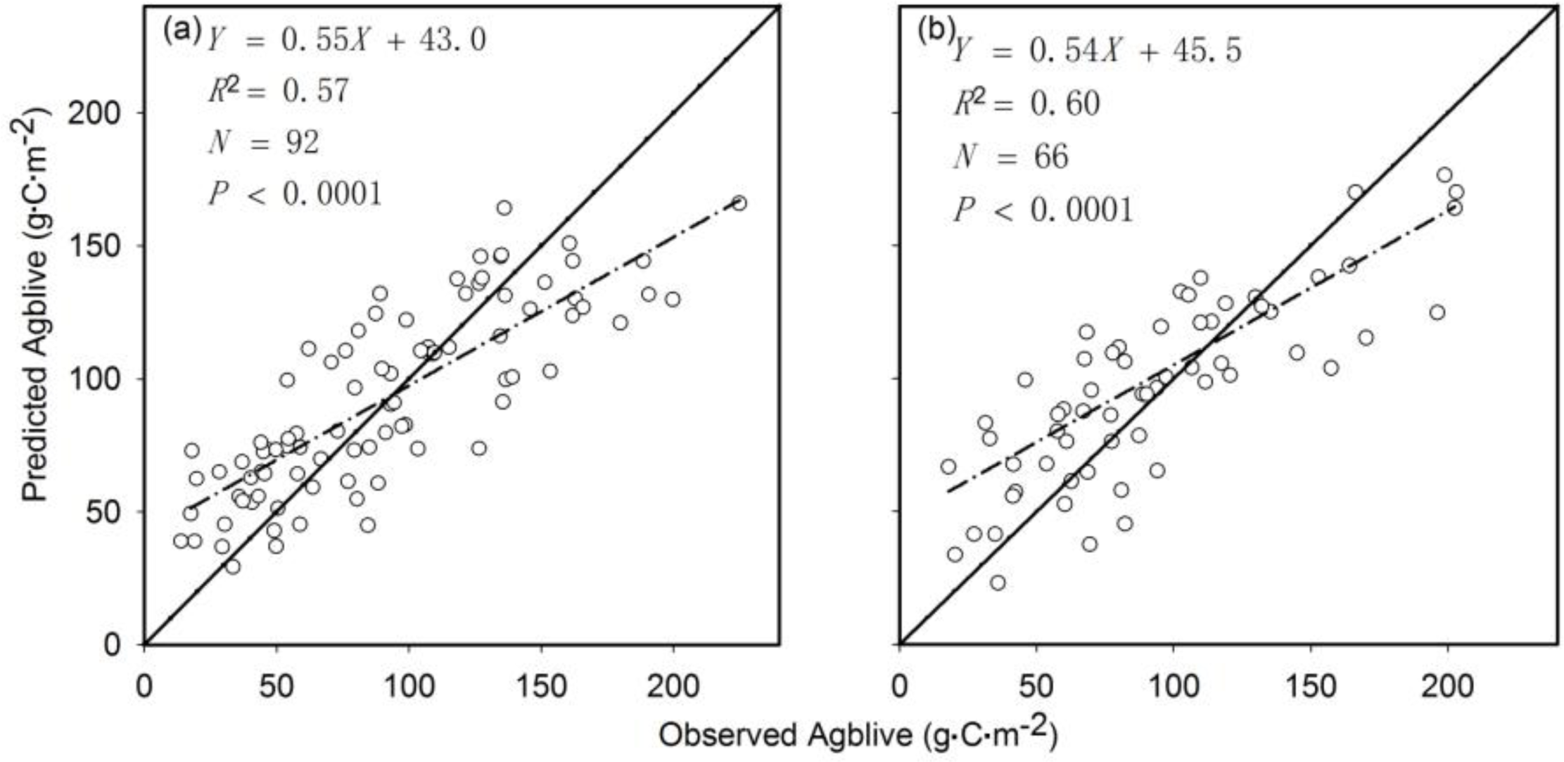
3.1. The Aboveground Live Biomass Model for Grassland Worldwide

The following grassland NDVI-biomass (GNB) model was found to be the best fit between aboveground live biomass carbon density (Agblive, g·C·m⁻²) for each pixel and its growing season average NDVI (NDVI_g) using the calibration dataset:

$$\mathit{Agblive}=52.2\times {{\mathit{NDVI}}_g}^2+173.9\times {\mathit{NDVI}}_g\hspace{0.17em}\hspace{0.17em}(R^2=0.57,P<0.0001),$$

(4)

Figure 2a shows that the GNB model explained about 57% of the observed variation of calibration data. The RMSE and RPE of the GNB model for the calibration dataset were 32.9 g·C·m⁻² and 2.2%, respectively. Figure 2b shows that the GNB model explained about 60% of the observed variation of the validation data. The RMSE and RPE of the GNB model for the validation dataset were 30.3 g·C·m⁻² and 5.5%, respectively.

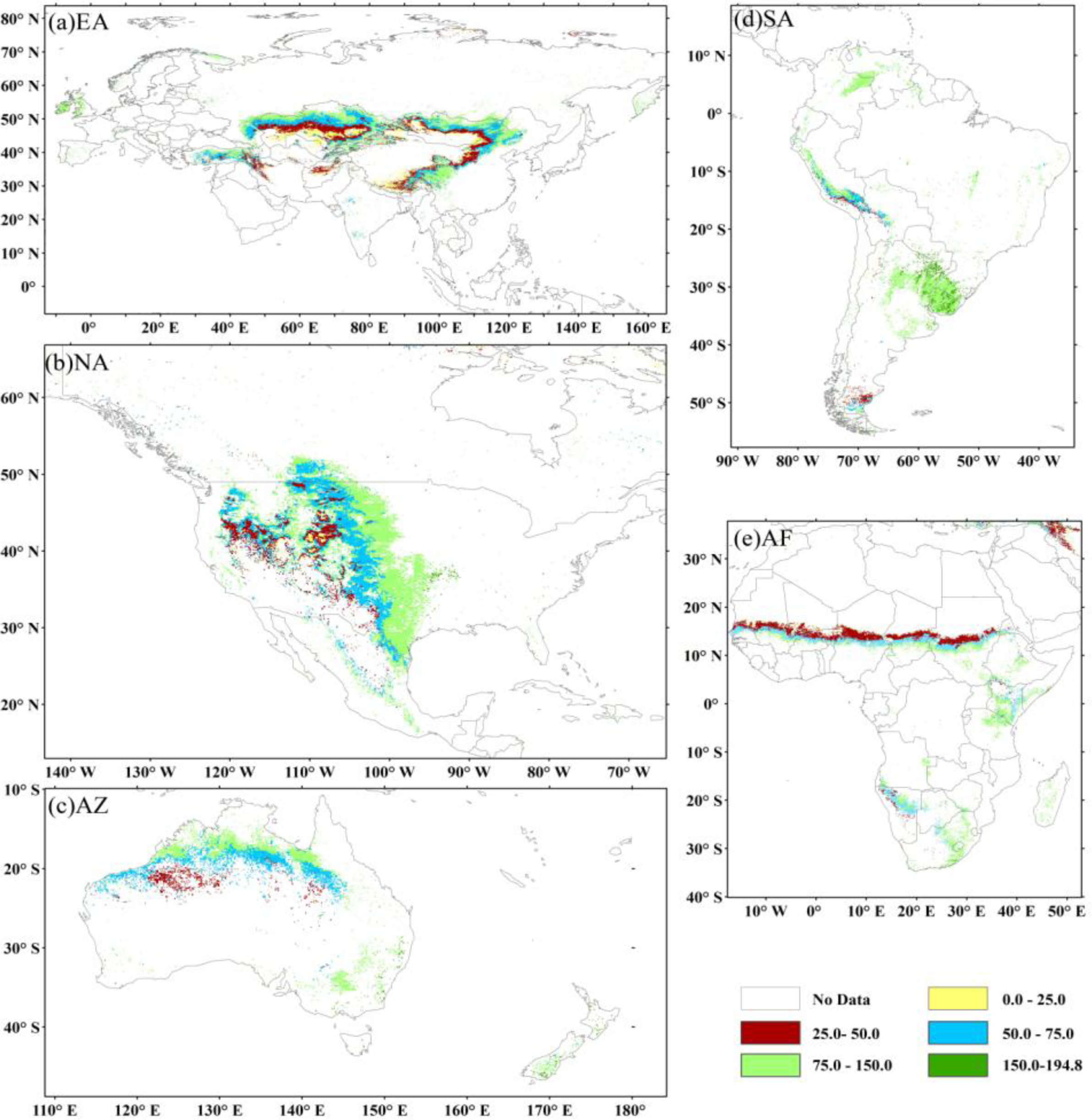
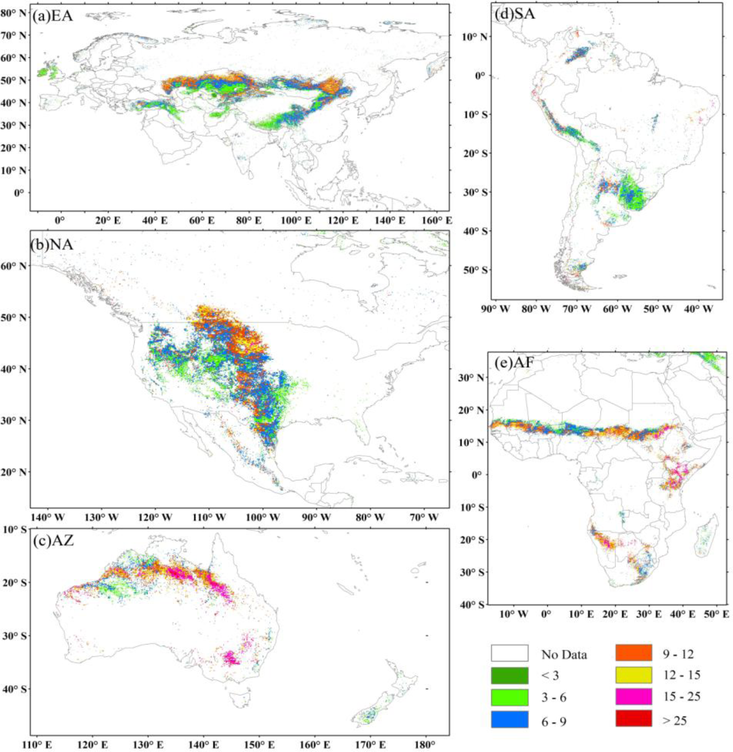
3.2. Global Biomass Carbon Stock and its Spatial Pattern

The average total annual aboveground live biomass carbon stock (Agbtc) of global grassland from 1982 to 2006 was 1051 Tg·C (i.e., 1.05 Pg·C) over a total area of 1.47 × 10⁷ km². EA, NA, AF, SA, and AZ contributed 41.7, 19.7, 17.8, 13.5, and 7.3% to the global Agbtc, respectively. Agblive increased with precipitation across the five regions (Figures 3 and S2 in the supplementary material). The lowest Agblive values (<25 g·C·m⁻², Figure 3a,b) appeared in dry regions, such as near deserts, and the highest values (>150 g·C·m⁻², Figure 3a,d) were found in humid regions such as SA and Europe.

3.3. Temporal Variability of Biomass Carbon Stock

The temporal variability of Agblive is an important indicator of the susceptibility of grassland to environmental stresses, such as drought. The higher the temporal variability, the more susceptible the grassland is to stresses. The temporal variability can be evaluated using standard deviation (STD) and coefficient of variation (CV) of the Agblive from 1982 to 2006. Results showed that the overall spatial pattern of STD resembled that of the mean Agblive (Figure 4). However, exceptions were found in eastern NA, Europe, and SA, where the STD was relatively low while mean Abglive was high. AZ had the largest STD and SA had the lowest among the regions. The spatial pattern of CV, opposite to that of STD, was signified by the coupling of high CV value with low biomass C density (Figure S3 in the supplementary material). The relatively low CV was found in eastern NA, Europe, and SA as they had low STD and high mean Agblive. The CV in AZ was found to be the highest among all regions.

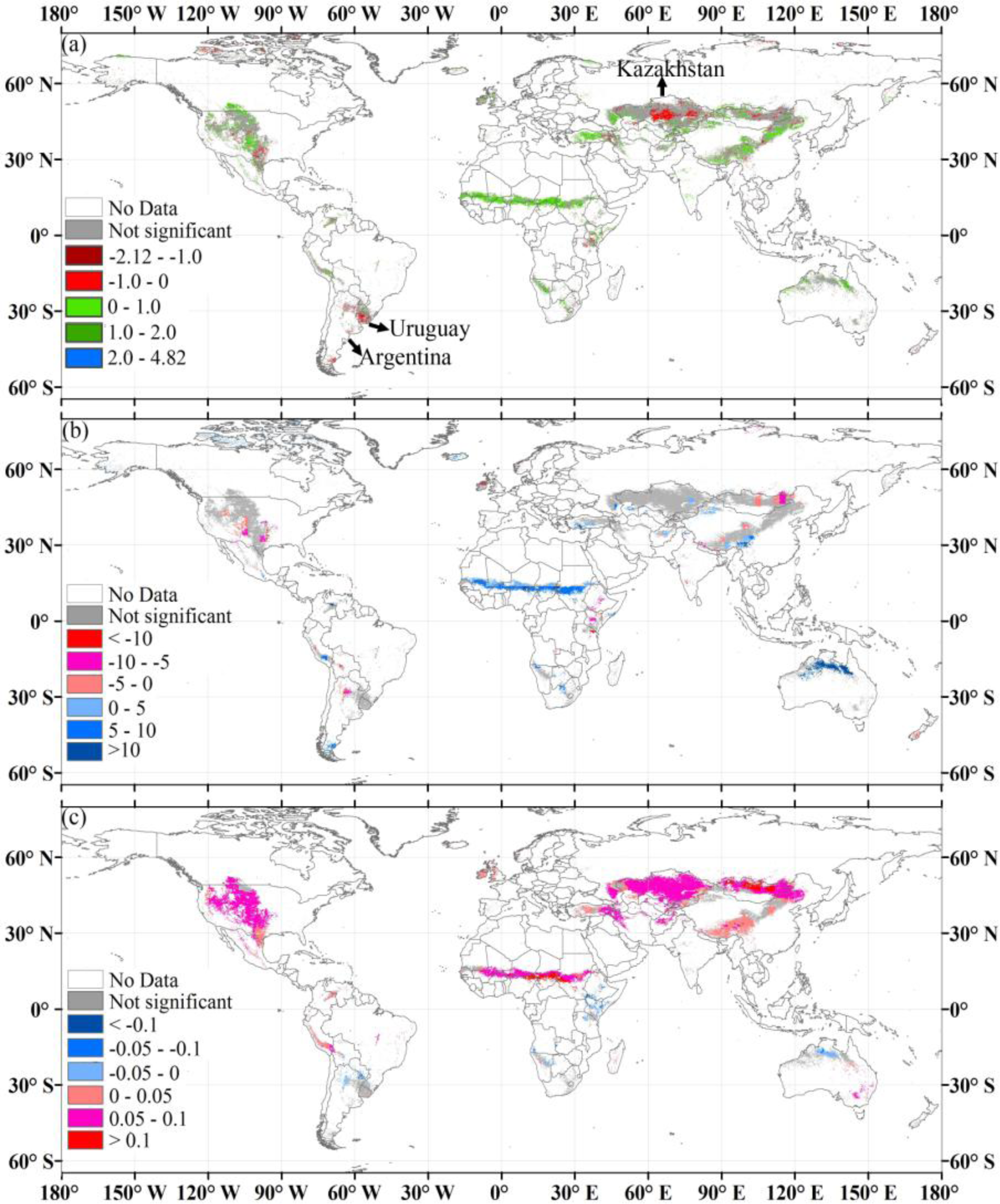
3.4. Temporal Trends of Biomass Carbon and Climate Change at Continental and Global Scales

Overall, the rate of change of global Agbtc was significant (P < 0.05), with an annual increasing rate of 2.43 Tg·C·yr⁻¹ during the study period (

Table 1. Grassland area, mean aboveground live biomass carbon density (Agblive, g·C·m⁻²), total C stock (1 Tg·C = 10¹² g·C), linear trends (Tg·C·yr⁻¹), and Pearson’s correlation coefficients of aboveground live biomass carbon from 1982 to 2006. Analysis of trends and correlations were performed for the entire period and by time segment. Turning point signifies a sudden change in trend between two time periods. R_t and R_p are the Pearson’s correlation coefficients between temperature and total C, and precipitation and total C, respectively. First and second time period refers to the time period before and after the turning point, respectively. As examples, the negative trends found in three countries (i.e., Argentina, Kazakhstan and Uruguay) are listed in the table, and their possible driving forces are described in the text.

Region	Overall Analysis (1982–2006)						Turning Point (year)	First Time Period			Second Time Period
	Area (104 km2)	Agblive (g·C·m−2)	Total C (Tg·C)	Trend (Tg·C·yr−1)	Rt	Rp		Trend (Tg·C·yr−1)	Rt	Rp	Trend (Tg·C·yr−1)	Rt	Rp
Global	1473.76	71.4	1051.71	2.43 **	0.52 **	0.54 **	1994	7.71 **	0.42	0.52	−2.17	0.13	0.39
EA	701.32	62.6	438.75	0.65	0.13	0.54 *	1994	5.03 **	0.23	0.68 *	−1.97 *	−0.33	0.42
AF	273.88	68.5	187.49	1.21 **	0.3	0.86 *	1994	2.0 *	−0.15	0.89 **	0.15	−0.27	0.72 *
NA	276.72	75.1	207.72	0.33 *	0.25	0.42 *	1993	0.87	0.03	0.61 *	−0.42	−0.29	0.51
SA	125.2	113.4	141.97	−0.04	−0.19	0.35	1997	0.2	−0.13	0.06	−0.93 **	0.003	0.6
AZ	96.64	78.4	75.79	0.29	−0.78 **	0.82 *	-	-	-	-	-	-	-
Kazakhstan	203.48	55.9	113.8	−0.13	−0.24	0.47 *	1993	2.14 **	−0.14	0.66 *	−1.57 **	−0.52	0.41
Uruguay	15	145.8	21.9	−0.03 *	−0.48 *	0.42 *	-	-	-	-	-	-	-
Argentina	40.1	120.3	48.4	−0.07	−0.24	0.38	1997	0.05	−0.42	0.16	−0.53 **	−0.08	0.66 *

Note:

^**:P < 0.01;

^*:P < 0.05.

). Meanwhile, the temporal pattern of change demonstrated obvious regional heterogeneity. Although the aboveground live biomass C in all five regions varied over time with either upward (positive) or downward trends, only the trends found in AF (1.21 Tg·C·yr⁻¹) and in NA (0.33 Tg·C·yr⁻¹) were positive and statistically significant during the study period.

Piecewise trend analysis showed two distinct periods globally in EA, AF, NA, and SA, but not in AZ (Table 1). The break or turning points of the trends appeared mostly around 1994. All significant trends before the break point were positive, and all significant trends were negative after the break point. At a global scale, the significantly positive trend of Agbtc before 1994 turned to negative afterwards (although not statistically significant). The change of trends in EA was the most obvious, from a significantly positive to a significantly negative trend before and after 1994, respectively. The significant positive trend of Agbtc in AF was stalled in 1994, and the insignificant trend of Agbtc in SA became significantly negative after 1997.

At continental and global scales, precipitation showed a significantly positive trend only in AF during the study period; however, temperature showed significantly positive trends globally in EA, AF, and NA (

Table 2. Annual precipitation (Pr, mm), mean temperature (Ta, °C), linear trends of annual precipitation, and mean temperature from 1982 to 2006. Analysis of trends was performed for the entire period and by time segment of aboveground live biomass carbon density in Table 1. T_Pr (mm·yr⁻¹) and T_Ta (°C·yr⁻¹) are the trends of annual precipitation and mean temperature, respectively. First and second time period refers to the time period before and after the turning point, respectively.

Region	Overall Analysis (1982–2006)				First Time Period		Second Time Period
	Pr (mm)	Ta (°C)	TPr (mm·yr−1)	TTa (°C·yr−1)	TPr (mm·yr−1)	TTa (°C·yr−1)	TPr (mm·yr−1)	TTa (°C·yr−1)
Global	558.8	12.4	0.81	0.04 **	1.05	0.04	0.24	0.05 **
EA	453.7	5.3	0.07	0.05 **	3.50	0.02	−0.19	0.06 *
AF	465.5	26.5	3.37 **	0.04 **	5.15	0.04	0.01	0.05 *
NA	522.7	9.3	−1.62	0.06 **	0.02	0.07	−5.59	0.09 **
SA	1294.4	18.3	−0.81	0.00	−7.48	0.02	−14.16	0.01
AZ	736.7	25.3	8.00	0.00	-	-	-	-

Note:

^**:P < 0.01;

^*:P < 0.05.

). Piecewise trends of precipitation and temperature were performed by the time segment of aboveground live biomass carbon density. Although the positive trends of precipitation became weak or turned to negative after the turning point, those trends were all insignificant. The positive trends of temperature were not significant before the turning point. After the turning point, the positive trends of temperature were significant and stronger than those for the entire study period at the global scale and for EA, AF, and NA.

3.5. Biomass, Climate, and Their Correlations at the Pixel Level

Spatial patterns of trends in Agblive, annual total precipitation, and mean temperature showed diverse patterns across the five regions (Figure 5). About 21.4, 21.8, 10.7, 50.0, and 22.4% of the grassland area experienced a significant increase in Agblive in NA, EA, SA, AF, and AZ, respectively (Figure 5a). In contrast, a smaller proportion of grassland showed significantly negative trends of Agblive with 10.1, 10.1, 18.2, 3.5, and 3.1%, respectively, for the five regions. Meanwhile, precipitation showed a significant increase over 58.7% and 50.9% of the grassland area in AF and AZ, but no obvious trends were detected for most of the grassland in NA, EA, and AZ (Figure 5b). A significant temperature increase was found over a majority (58.9%–91.9%) of the grasslands in NA, EA, and AF (Figure 5c). In contrast, only 27.6% of the grassland in SA demonstrated significantly positive trends of temperature, and 17.0% showed negative trends (about 17.0%, Figure 5c). The areas with positive and negative trends of temperature were equal in AZ (about 19%, Figure 5c).

Spatial patterns of correlation between Agblive carbon density and climate variables showed distinct regional differentiation. The area fraction with significantly positive correlation between Agblive and precipitation varied across regions with 74.9% in AF, 79.6% in AZ, 36% in NA, 35% in EA, and 19% in SA (Figure 6a). Agblive and temperature showed a significantly negative relationship over 73% of the grassland area in AZ (Figure 6b). The highest fraction of grassland with a significantly positive correlation between Agblive and temperature was found in AF with 27.1% (Figure 6b). Interestingly, a negative correlation between Agblive and temperature was found in places where the Agblive showed negative trends in NA, EA, and SA (Figures 5a and 6b).

The correlations between global Agbtc and two climate variables (i.e., precipitation and temperature) from 1982 to 2006 were similar (Table 1). The piecewise analysis showed weakened correlations compared with the results for the entire period. Significantly positive correlations between Agbtc and precipitation were found for all regions except SA, which might be explained by the abundance of precipitation in the region. The correlations between Agbtc and temperature were not significant regionally except the negative correlation found in AZ. The correlations of Agbtc and climate variables showed various changes after breaking the study period into two time segments (Table 1). Both the significant biomass-temperature and biomass-precipitation correlations at the global scale became insignificant after the break; the biomass-temperature correlations remained insignificant. The biomass-precipitation correlations for the first time segments were stronger than those for the entire study period for EA, AF, and NA and remained significant after the break point only in AF.

4. Discussion

4.1. Evaluation of the Biomass Carbon Density Model

The validation of the model showed that the performance of the GNB model is robust and stable (Figure 2). The Agblive at the validation sites in this study was comparable with the estimates of the CENTURY model by Parton et al. [38]. Our validation sites include all the validation sites used in Parton’s study. The coefficient of determination (R² = 0.57 to 0.60) in this study falls in the range of the CENTURY results (R² = 0.45 to 0.65). It should be noted that the CENTURY model is a prognostic model that extensively uses site-specific information (e.g., soil properties, land use and management practices, and climate variables) but does not use satellite-derived spatial information such as NDVI. In contrast, the GNB model only uses NDVI. The good agreement between the GNB model and the CENTURY model suggests these two models were comparable in estimating grassland biomass. The GNB model is simpler and easier to use than process-based biogeochemical models such as CENTURY because these models usually require many site-specific parameters. Invariant parameters of the GNB model developed in this study make the model ideal for mapping the spatial and temporal changes of Agblive across various grassland types and geographical regions. In addition, the model itself and/or the continuous mapped fields of Agblive can be used as independent algorithms or constraints to compare with biogeochemical models at region or global scales.

NDVI was the only predictor in the grassland biomass model developed in this study. This becomes convenient and valuable for mapping biomass dynamics at regional to global scales as NDVI can be readily calculated from satellite observations. Although NDVI synoptically integrates the impacts of a suite of environmental factors (e.g., precipitation and temperature) and management practices on grassland biomass production [39,40], the GNB model did not perform well in both sparse and dense vegetated areas (Figure 2). Adding variables such as precipitation, temperature, and grazing intensity might help reduce the biases in these under-performing regions in the future. Unfortunately, we were unable to perform this analysis because such information was not available for most of the sites in our dataset.

4.2. Comparison of Biomass Estimates

Our estimates are comparable with previous estimates of grassland biomass at global and regional scales. Previous estimates of global grassland biomass were primarily on total aboveground biomass (AGB), which includes aboveground live biomass (Agblive), standing dead (Agbstdead), and litter (Agblitter). In order to compare with these estimates, we calculated AGB as the sum of the standing dead and litter using the statistical models built from our dataset (i.e., Agbstdead = 1.0 × Agblive − 16.7, R² = 0.48, P < 0.05; Agblitter = 0.66 × Agblive + 13.7, R² = 0.46, P < 0.05). The estimated average AGB density for the grasslands was 186.9 g·C·m⁻², comparable with the density estimate of 170.3 g·C·m⁻² from Jackson et al. [41] for temperate grasslands worldwide. The average Agblive in China estimated from this study was 59.7 g·C·m⁻², higher than the estimates of 43.5 g·C·m⁻² by Piao et al. [14] and 47.2 g·C·m⁻² by Yang et al. [15]. To investigate the reasons behind the difference, we compared the GNB model with Piao’s model in northern China and found that the performance of the GNB model (R² = 0.70, P < 0.05, RMSE = 24.1 g·C·m⁻²) was very close to Piao’s model (R² = 0.70, P < 0.05, RMSE = 24.0 g·C·m⁻²). The discrepancy of Agblive estimates between these studies might be caused by the differences in underlying grassland maps. Piao’s study [14] used a different grassland map that included temperate desert, high-cold desert-steppe, tropical grassland, and lowland grassland whereas the MODIS map did not have these categories.

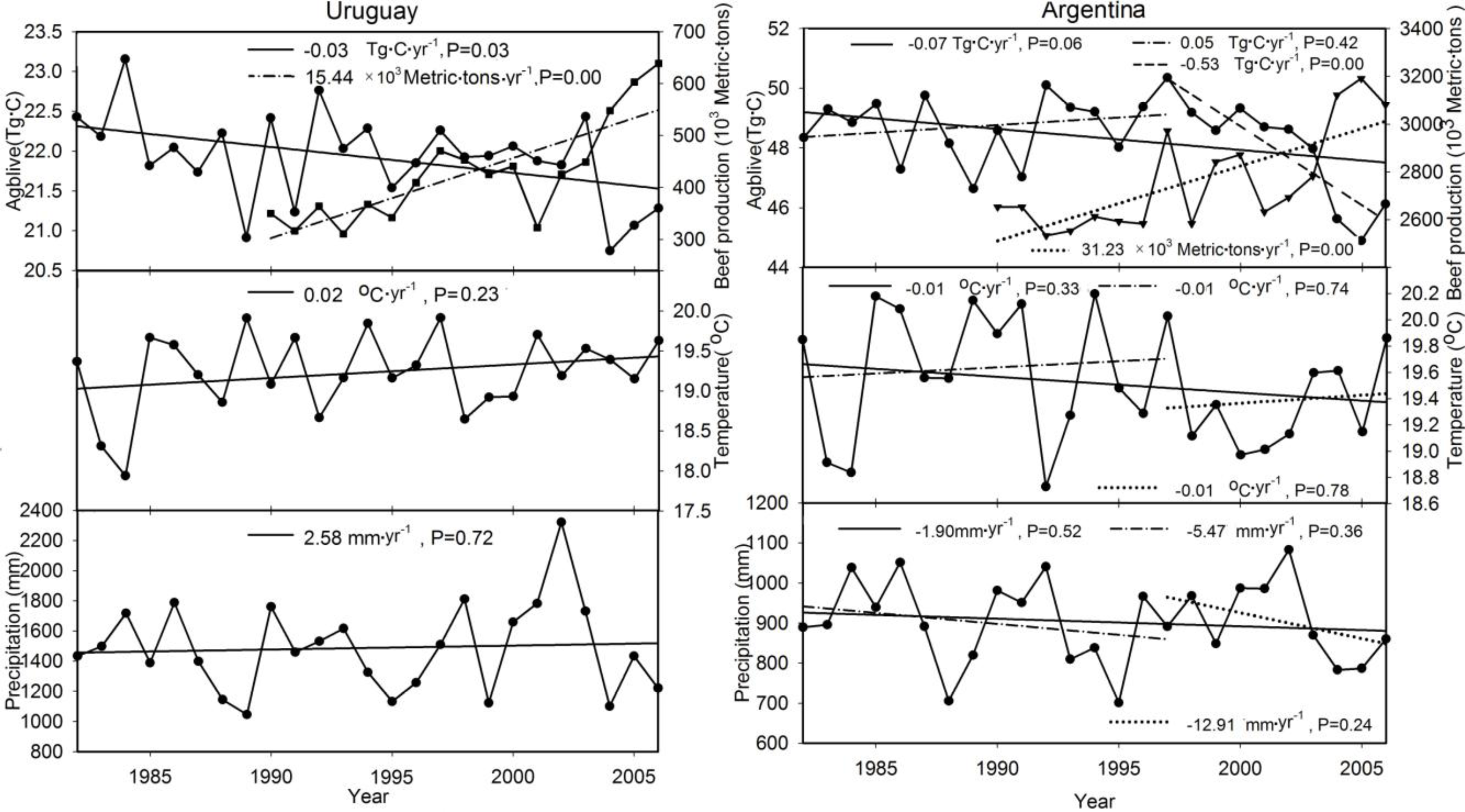
4.3. Controlling Factors of Biomass Carbon Change

Globally, we can characterize the biomass C stock in the five regions into three levels: low (EA and AF with a mean Agblive value of 64.2 g·C·m⁻²), medium (NA and AZ with a mean value of about 75.9 g·C·m⁻²), and high (SA with a mean value of 113.4 g·C·m⁻²). This gradient of biomass stock follows the mean annual precipitation gradient that ranges from low (453.7 mm for EA and 465.5 mm for AF), medium (524.6 mm for NA and 736.7 mm for AZ), to high (1,294.4 mm for SA). The Agblive across the five regions showed a strong positive correlation with annual mean precipitation (R² = 0.96, P < 0.05). The fact that grassland biomass carbon was mainly controlled by precipitation across the five regions was consistent with previous studies [17,19,20].

The interannual variability of grassland biomass was mainly controlled by precipitation during the period of 1982–2006 because precipitation explained 42–86% of the temporal variance of grassland biomass change (Table 1). However, the influence of precipitation became weaker after the turning points. The effect of temperature trend on grassland biomass change was not straightforward, depending on its interaction with precipitation [42]. Although temperature change over time was significantly and negatively correlated with precipitation at most of the grassland areas in NA, Australia, and Southern Africa (Figure S4 in the supplementary material), grassland growth trends demonstrated diverse regional patterns (

Table 3. Regional examples of association of the changes in precipitation, temperature, and aboveground biomass carbon.

Precipitation Trend	Temperature Trend	Biomass C Trend	Regions
decrease	increase	Decrease	Southern Oklahoma, Central Texas, USA
increase	decrease	None	Northern Territory of Australia
increase	none	Increase	Southern Africa and Western Australia and Queensland of Australia
none	increase	Decrease	Central and Eastern Kazakhstan
increase	increase	Increase	Sahel region of Africa

and Figure 5). The underlying mechanisms for these diverse trends varied. For example, increasing temperature might increase the consumptive use of soil moisture via enhanced evapotranspiration and thus reduce available soil moisture for plant growth. This might explain the decrease of biomass in Central and Eastern Kazakhstan where temperature increased but precipitation remained unchanged. Increasing temperature did not necessarily lead to the decrease of biomass as the negative temperature effect could be offset or overpowered by the positive effect of increased precipitation (e.g., Sahel region of Africa). Decreasing precipitation compounded by increasing temperature has led to the observed decrease of grassland biomass in the Southwestern United States, especially in Southern Oklahoma and Central Texas. Apparently, there is a need for further investigation of the diverse grassland responses to the complex interaction between precipitation and temperature.

As the Agbtc of EA and AF account for 60% of global Agbtc, the turning point (i.e., 1994) of global Agbtc is the same with EA and AF. The turning point of Agbtc in AF could be explained by precipitation as their significant positive correlation (Table 1). The change of precipitation in AF may be affected by El Niño/Southern Oscillation (ENSO) [43]. The AF showed a drop in precipitation in 1984 during ENSO cold year, and a peak in precipitation in 1988 and 1994 during ENSO cold and warm years. The Agbtc in AF showed the same change with precipitation in the ENSO years (Figure S5). The significant decrease trend of Agbtc in EA after 1994 could not be explained by precipitation as their correlations were not significant (Table 1 and Figure S6). Although the negative correlation between the Agbtc and temperature was not significant, the significant increased temperature may suppress grassland biomass through influencing water availability [42,44].

In addition to climate variables, some other factors might affect biomass change at least regionally. For example, a significant negative trend of Agblive was found in Argentina and Uruguay (Figure 5a). The decreased grassland aboveground live biomass in Argentina and Uruguay may be partly caused by increasing beef production. As of 2007, 80–90% of beef production was grass fed in these two countries. According to the data from Mathews and Vandeveer [45], beef production increased significantly from 1990 to 2006 in Uruguay (15,441 metric·tons·yr⁻¹, P < 0.05) and in Argentina (31,238 metric·tons·yr⁻¹, P < 0.05) (Figure 7). Beef production in both countries showed significantly negative correlations with aboveground live biomass carbon stock (Argentina: R = −0.68, P < 0.05; Uruguay: R = −0.50, P < 0.05) from 1990–2006. For EA, the grassland ecosystems in the Inner Mongolia of China and Mongolia have been degraded under the influence of both climate change and intensified human activities (such as overgrazing to meet the regional demand for meat and grassland conversion to croplands) [46]. Those results suggested that management practices (such as grazing for meat production) should be considered in the impact factor analysis of global grassland biomass change.

4.4. Uncertainties

In this study, we have quantified the spatial and temporal changes of aboveground biomass carbon stocks of global grasslands from 1982 to 2006. Although we did not estimate the error limits of the estimates, making some general and qualitative observations on uncertainty can be helpful for future research. First, uncertainties exist in field measurements mainly from imbalanced geographic distribution of field sites (Figure 1). Second, an NDVI time series dataset may still contain errors from incomplete corrections of satellite drift and atmospheric effects. Third, the grassland distribution map was static, which might not be able to reflect the quick response of grassland to interannual change of precipitation as some research has indicated in the transition zones between deserts and dry grassland in Sahel, Africa [47]. To overcome those uncertainties, future efforts should be tailored to increase observation sites, balance geographic distribution of field studies, and take advantage of advances in remote sensing.

5. Summary

Using a worldwide grassland biomass measurements dataset, remote sensing NDVI, and climate reanalyzed data, we quantified for the first time the spatio-temporal patterns of biomass carbon stock of global grassland ecosystems and analyzed major controlling factors at a spatial resolution of ∼8 km during the period 1982–2006. The average aboveground carbon stock in the global grassland ecosystem for 1982–2006 was 1.05 Pg·C. The carbon storage increased over the study period with a rate of 2.43 Tg·C·y⁻¹. Two distinct periods were found in the trends of the total aboveground live biomass carbon stock globally and across EA, NA, SA, and AF. Globally, the change of biomass was significantly and positively correlated with temperature and precipitation. Regionally, biomass carbon density can be divided into low (EA and AF), medium (NA and AZ), and high (SA) levels, following the precipitation gradient across these regions. In addition to climate factors, disturbances and management practices (such as grazing for meat production) should be considered in the impact factor analysis of global grassland biomass change.

remotesensing-06-01783-s001.pdf

References

1. Hall, D.O.; Scurlock, J.M.O. Climate change and productivity of natural grasslands. Ann. Bot 1991, 67, 49–55. [Google Scholar]
2. Scurlock, J.M.O; Hall, D.O. The global carbon sink: A grassland perspective. Glob. Chang. Biol 1998, 4, 229–233. [Google Scholar]
3. Ma, W.; Fang, J.; Yang, Y.; Mohammat, A. Biomass carbon stocks and their changes in northern China’s grasslands during 1982–2006. Sci. China Life Sci 2010, 53, 841–850. [Google Scholar]
4. Canadell, J.G.; Le Quéré, C.; Raupach, M.R.; Field, C.B.; Buitenhuis, E.T.; Ciais, P.; Conway, T.J.; Gillett, N.P.; Houghton, R.A.; Marland, G. Contributions to accelerating atmospheric CO2 growth from economic activity, carbon intensity, and efficiency of natural sinks. Proc. Natl. Acad. Sci. USA 2007, 104, 18866–18870. [Google Scholar]
5. Kruska, R.L.; Reid, R.S.; Thornton, P.K.; Henninger, N.; Kristjanson, P.M. Mapping livestock-oriented agricultural production systems for the developing world. Agric. Syst 2003, 77, 39–63. [Google Scholar]
6. Thornton, P.K.; van de Steeg, J.; Notenbaert, A.; Herrero, M. The impacts of climate change on livestock and livestock systems in developing countries: A review of what we know and what we need to know. Agric. Syst 2009, 101, 113–127. [Google Scholar]
7. Sautier, M.; Martin-Clouaire, R.; Faivre, R.; Duru, M. Assessing climatic exposure of grassland-based livestock systems with seasonal-scale indicators. Clim. Chang 2013, 120, 1–15. [Google Scholar]
8. Jones, M.B.; Donnelly, A. Carbon sequestration in temperate grassland ecosystems and the influence of management, climate and elevated CO2. New Phytol 2004, 164, 423–439. [Google Scholar]
9. Sala, O.E.; Gherardi, L.A.; Reichmann, L.; Jobbágy, E.; Peters, D. Legacies of precipitation fluctuations on primary production: Theory and data synthesis. Philos. Trans. R. Soc. B. Biol. Sci 2012, 367, 3135–3144. [Google Scholar]
10. Reichmann, L.G.; Sala, O.E.; Peters, D.P.C. Precipitation legacies in desert grassland primary production occur through previous-year tiller density. Ecology 2013, 94, 435–443. [Google Scholar]
11. Tucker, C.J.; Vanpraet, C.L.; Sharman, M.J.; van Ittersum, G. Satellite remote sensing of total herbaceous biomass production in the Senegalese Sahel: 1980–1984. Remote Sens. Environ 1985, 17, 233–249. [Google Scholar]
12. Wylie, B.K.; Meyer, D.J.; Tieszen, L.L.; Mannel, S. Satellite mapping of surface biophysical parameters at the biome scale over the North American grasslands: A case study. Remote Sens. Environ 2002, 79, 266–278. [Google Scholar]
13. Asner, G.P.; Nepstad, D.; Cardinot, G.; Ray, D. Drought stress and carbon uptake in an Amazon forest measured with spaceborne imaging spectroscopy. Proc. Natl. Acad. Sci. USA 2004, 101, 6039–6044. [Google Scholar]
14. Piao, S.; Fang, J.; Zhou, L.; Tan, K.; Tao, S. Changes in biomass carbon stocks in China’s grasslands between 1982 and 1999. Glob. Biogeochem. Cycles 2007. [Google Scholar] [CrossRef]
15. Yang, Y.; Fang, J.; Ma, W.; Guo, D.; Mohammat, A. Large-scale pattern of biomass partitioning across China’s grasslands. Glob. Ecol. Biogeogr 2010, 19, 268–277. [Google Scholar]
16. Ferreira, L.G.; Fernandez, L.E.; Sano, E.E.; Field, C.; Sousa, S.B.; Arantes, A.E.; Araújo, F.M. Biophysical properties of cultivated pastures in the Brazilian savanna biome: An analysis in the spatial-temporal domains based on ground and satellite data. Remote Sens 2013, 5, 307–326. [Google Scholar]
17. Sala, O.E.; Parton, W.J.; Joyce, L.A; Lauenroth, W.K. Primary production of the central grassland region of the United States. Ecology 1988, 69, 40–45. [Google Scholar]
18. McNaughton, S.J.; Sala, O.E.; Oesterheld, M. Comparative Ecology of African and South American Arid to Subhumid Ecosystems. In Biological Relationships between Africa and South America; Goldblatt, P., Ed.; Yale University Press: New Haven, CT, USA, 1993; pp. 548–567. [Google Scholar]
19. Briggs, J.M.; Knapp, A.K. Interannual variability in primary production in tallgrass prairie: Climate, soil moisture, topographic position, and fire as determinants of aboveground biomass. Am. J. Bot 1995, 1024–1030. [Google Scholar]
20. Bai, Y.; Wu, J.; Xing, Q.; Pan, Q.; Huang, J.; Yang, D.; Han, X. Primary production and rain use efficiency across a precipitation gradient on the Mongolia plateau. Ecology 2008, 89, 2140–2153. [Google Scholar]
21. Lauenroth, W.K.; Sala, O.E. Long-term forage production of North American shortgrass steppe. Ecol. Appl 1992, 2, 397–403. [Google Scholar]
22. Huxman, T.E.; Smith, M.D.; Fay, P.A.; Knapp, A.K.; Shaw, M.R.; Loik, M.E.; Smith, S.D.; Tissue, D.T.; Zak, J.C.; Weltzin, J.F.; et al. Convergence across biomes to a common rain-use efficiency. Nature 2004, 429, 651–654. [Google Scholar]
23. Hu, Z.; Fan, J.; Zhong, H.; Yu, G. Spatio-temporal dynamics of aboveground primary productivity along a precipitation gradient in Chinese temperate grassland. Sci. China Ser. D: Earth Sci 2007, 50, 754–764. [Google Scholar]
24. Herrmann, S.M.; Anyamba, A.; Tucker, C.J. Recent trends in vegetation dynamics in the African Sahel and their relationship to climate. Glob. Environ. Chang 2005, 15, 394–404. [Google Scholar]
25. Scurlock, J.M.O.; Johnson, K.R.; Olson, R.J. NPP Grassland: NPP Estimates from Biomass Dynamics for 31 Sites, 1948–1994; Oak Ridge National Laboratory Distributed Active Archive Center: Oak Ridge, TN, USA. Available online: http://www.daac.ornl.gov (accessed on 4 February 2003).
26. Olson, J.S.; Watts, J.A.; Allison, L.J. Carbon in Live Vegetation of Major World Ecosystem; Oak Ridge National Laboratory: Oak Ridge, TN, USA, 1983; p. 61. [Google Scholar]
27. Fang, J.; Guo, Z.; Piao, S.; Chen, A. Terrestrial vegetation carbon sinks in China, 1981–2000. Sci. China Ser. D: Earth Sci 2007, 50, 1341–1350. [Google Scholar]
28. Tucker, C.J.; Pinzon, J.E.; Brown, M.E.; Slayback, D.A.; Pak, E.W.; Mahoney, R.; Vermote, E.F.; El Saleous, N. An extended AVHRR 8-km NDVI dataset compatible with MODIS and SPOT vegetation NDVI data. Int. J. Remote Sens 2005, 26, 4485–4498. [Google Scholar]
29. Holben, B.N. Characteristics of maximum-value composite images from temporal AVHRR data. Int. J. Remote Sens 1986, 7, 1417–1434. [Google Scholar]
30. Global Modeling and Assimilation Office, File Specification for GEOSDAS Gridded Output Version 5.3; NASA Goddard Space Flight Cent: Greenbelt, MD, USA, 2004.
31. Yuan, W.; Liu, S.; Yu, G.; Bonnefond, J.-M.; Chen, J.; Davis, K.; Desai, A.R.; Goldstein, A.H.; Gianelle, D.; Rossi, F.; et al. Global estimates of evapotranspiration and gross primary production based on MODIS and global meteorology data. Remote Sens. Environ 2010, 114, 1416–1431. [Google Scholar]
32. Adler, R.F.; Huffman, G.J.; Chang, A.; Ferraro, R.; Xie, P.-P.; Janowiak, J.; Rudolf, B.; Schneider, U.; Curtis, S.; Bolvin, D.; et al. The version-2 global precipitation climatology project (GPCP) monthly precipitation analysis (1979–present). J. Hydrometeorol 2003, 4, 1147–1167. [Google Scholar]
33. Rienecker, M.M.; Suarez, M.J.; Gelaro, R.; Todling, R.; Bacmeister, J.; Liu, E.; Bosilovich, M.G.; Schubert, S.D.; Takacs, L.; Kim, G.-K.; et al. MERRA: NASA’s modern-era retrospective analysis for research and applications. J. Clim 2011, 24, 3624–3648. [Google Scholar]
34. Zhang, K.; Kimball, J.S.; Mu, Q.; Jones, L.A.; Goetz, S.J.; Running, S.W. Satellite based analysis of northern ET trends and associated changes in the regional water balance from 1983 to 2005. J. Hydrol 2009, 379, 92–110. [Google Scholar]
35. Fensholt, R.; Rasmussen, K. Analysis of trends in the Sahelian “rain-use efficiency” using GIMMS NDVI, RFE and GPCP rainfall data. Remote Sens. Environ 2011, 115, 438–451. [Google Scholar]
36. Chatterjee, S.; Hadi, A.S. Influential observations, high leverage points, and outliers in linear regression. Stat. Sci 1986, 1, 379–393. [Google Scholar]
37. Toms, J.D.; Lesperance, M.L. Piecewise regression: A tool for identifying ecological thresholds. Ecology 2003, 84, 2034–2041. [Google Scholar]
38. Parton, W.J.; Scurlock, J.M.O.; Ojima, D.S.; Gilmanov, T.G.; Scholes, R.J.; Schimel, D.S.; Kirchner, T.; Menaut, J.-C.; Seastedt, T.; Garcia Moya, E.; et al. Observations and modeling of biomass and soil organic matter dynamics for the grassland biome worldwide. Glob. Biogeochem. Cycle 1993, 7, 785–809. [Google Scholar]
39. Kawamura, K.; Akiyama, T.; Yokota, H.-O.; Tsutsumi, M.; Yasuda, T.; Watanabe, O.; Wang, S. Quantifying grazing intensities using geographic information systems and satellite remote sensing in the Xilingol steppe region, Inner Mongolia, China. Agric. Ecosyst. Environ. 2005, 107, 83–93. [Google Scholar]
40. Blanco, L.J.; Aguilera, M.O.; Paruelo, J.M.; Biurrun, F.N. Grazing effect on NDVI across an aridity gradient in Argentina. J. Arid Environ 2008, 72, 764–776. [Google Scholar]
41. Jackson, R.B.; Canadell, J.; Ehleringer, J.R.; Mooney, H.A.; Sala, O.E.; Schulze, E.D. A global analysis of root distributions for terrestrial biomes. Oecologia 1996, 108, 389–411. [Google Scholar]
42. Bradford, J.B.; Lauenroth, W.K.; Burke, I.C.; Paruelo, J.M. The influence of climate, soils, weather, and land use on primary production and biomass seasonality in the US Great Plains. Ecosystems 2006, 9, 934–950. [Google Scholar]
43. Anyamba, A.; Tucker, C.J. Analysis of Sahelian vegetation dynamics using NOAA-AVHRR NDVI data from 1981–2003. J. Arid Environ 2005, 63, 596–614. [Google Scholar]
44. John, R.; Chen, J.; Ou-Yang, Z.-T.; Xiao, J.; Becker, R.; Samanta, A.; Ganguly, S.; Yuan, W.; Batkhishig, O. Vegetation response to extreme climate events on the Mongolian Plateau from 2000 to 2010. Environ. Res. Lett 2013. [Google Scholar] [CrossRef]
45. Mathews, K.H., Jr.; Vandeveer, M. Beef Production, Markets, and Trade in Argentina and Uruguay: An Overview; United States Department of Agriculture: Washington, DC, USA, 2007. [Google Scholar]
46. Qi, J.; Chen, J.; Wan, S.; Ai, L. Understanding the coupled natural and human systems in dryland East Asia. Environ. Res. Lett 2012. [Google Scholar] [CrossRef]
47. Tucker, C.J.; Nicholson, S.E. Variations in the size of the Sahara Desert from 1980 to 1997. Ambio 1999, 28, 587–591. [Google Scholar]
Figure 1. Map showing locations of the 81 field plots of aboveground live biomass (Agblive) measurements used for model calibration and validation. The inset shows the frequency distribution of field sites in the five regions.
Remotesensing 06 01783f1
Figure 2. Comparison of the predicted and observed aboveground live biomass carbon density (Agblive) at calibration (a) and validation (b) sites. The solid line is the 1:1 line and the short dashed line is the linear regression line.
Remotesensing 06 01783f2
Figure 3. Spatial patterns of multiyear (1982–2006) mean aboveground live biomass carbon density (Agblive, g·C·m−2) in the five regions (i.e., (a) Europe and Asia (EA), (b) North America (NA), (c) Australia and New Zealand (AZ), (d) South America (SA), and (e) Africa (AF)).
Remotesensing 06 01783f3
Figure 4. Spatial patterns of standard deviation (STD, g·C·m−2) of the simulated aboveground live biomass carbon density in the five regions (i.e., (a) Europe and Asia (EA), (b) North America (NA), (c) Australia and New Zealand (AZ), (d) South America (SA), and (e) Africa (AF)) from 1982 to 2006.
Remotesensing 06 01783f4
Figure 5. Spatial patterns of trends of aboveground biomass carbon density ((a), gC·m−2·year−1), annual precipitation ((b), mm·year−1) and mean temperature ((c),°C·year−1) from 1982 to 2006.
Remotesensing 06 01783f5
Figure 6. Pearson’s correlation coefficients between annual precipitation and aboveground biomass carbon density (a), and between annual mean temperature and aboveground biomass carbon density (b).
Remotesensing 06 01783f6
Figure 7. Interannual variability of total aboveground live biomass carbon stock (Tg·C·yr−1), beef production (Metric·tons·yr−1), annual mean temperature (°C·yr−1), and precipitation (mm·yr−1) in Uruguay (Left) and Argentina (Right).
Remotesensing 06 01783f7