Classification of Plot-Level Fire-Caused Tree Mortality in a Redwood Forest Using Digital Orthophotography and LiDAR

Abstract

Aerial and satellite imagery are widely used to assess the severity and impact of wildfires. Light detection and ranging (LiDAR) is a newer remote sensing technology that has demonstrated utility in measuring vegetation structure. Combined use of imagery and LiDAR may improve the assessment of wildfire impacts compared to imagery alone. Estimation of tree mortality at the plot scale could serve for more rapid, broad-scale, and lower cost post-fire assessments than feasible through field assessment. We assessed the accuracy of classifying color-infrared imagery in combination with post-fire LiDAR, and with differenced (pre- and post-fire) LiDAR, in estimating plot percent mortality in a second-growth coast redwood forest near Santa Cruz, CA. Percent mortality of trees greater than 25.4 cm DBH in 47 permanent 0.08 ha plots was categorized as low (<25%), moderate (25%–50%), or high (>50%). The model using Normalized Difference Vegetation Index (NDVI) from National Agricultural Imagery Program (NAIP) was 74% accurate; the model using NDVI and post-fire LiDAR was 85% accurate, while the model using NDVI and differenced LiDAR was 83% accurate. The addition of post-fire LiDAR data provided a modest increase in accuracy compared to imagery alone, which may not justify the substantial cost of data acquisition. The method demonstrated could be applied to rapidly estimate tree mortality resulting from wildfires at fine to moderate scale.

1. Introduction

Wildland fires burn with varying intensity, which may be measured as flame height, heat, rate of spread, or total energy released. The resulting ecological effects depend on the interaction of intensity, duration and landscape characteristics, and are commonly referred to as fire severity, a broad term which encompasses mortality of vegetation as well as change in cover, effects on soil, and other factors. One field measurement of burn severity which is applicable across a wide range of vegetation types and has gained relatively widespread acceptance is composite burn index (CBI). CBI rating comprises the condition and color of soil, amount of vegetation consumed, scorch of trees, and presence of sprouting and/or new colonizing vegetation [1]. While useful, estimates of severity are not generally sufficient to make stand-level forest management decisions about post-fire response. Forest managers in particular have a need for information about fire effects and the spatial distribution of tree mortality following wildfire, but direct assessment from the field is time-consuming and costly. Remote sensing may be used to estimate varying levels of mortality and provide a more efficient, timely, scalable, and potentially more cost-effective means for post-fire assessment. The changes to the structure and color of aboveground vegetation and the color of soil following wildfire result in changes in the signal returned by both active and passive remote sensing systems. In particular, discrete-return light detection and ranging (LiDAR) and digital orthophotography (imagery) are commonly used to assess the condition of vegetation, including change detection following disturbance events such as wildland fire.

Between the two technologies, the use of imagery to detect and characterize tree mortality and severity of forest fires has a more well-developed and robust research history. CBI was developed for the purpose of relating ground-based estimates of burn severity to estimates derived from 30 m resolution Landsat TM/ETM imagery [1]. Common image processing methods used to characterize burn severity include linear transformations, univariate image differencing, and supervised, unsupervised, and hybrid classification; the most commonly used strategies are methods of univariate image differencing [2]. Commonly used indices based on band ratios are the normalized burn ratio (NBR) and the normalized difference vegetation index (NDVI), and the differenced versions, dNBR and dNDVI. Although dNBR may be more sensitive to changes caused by wildland fire, dNDVI can be calculated from more commonly available color infrared imagery, which may also be available at finer spatial and temporal scales than Landsat imagery. Comparison of NDVI, NBR, dNDVI, and dNBR from Landsat TM/ETM+ scenes across four wildfire burn sites in Alaska to CBI found that NDVI performed similarly to NBR (|r| of 0.72 vs. 0.77) and dNDVI similarly to dNBR (|r| of 0.67 vs. 0.70) [3]. Assessment of fire severity across three fires in pine, oak, and eucalyptus forests in Spain found that NDVI performed similarly to NBR, dNDVI similarly to dNBR, and that single-scene indices outperformed multi-temporal indices at describing severity within burned areas, while multi-temporal indices were more accurate at distinguishing between burned and unburned areas [4]. With any method based on imagery, accuracy can be an issue, as “countervailing post-fire factors often lead to spectral confusion” [5].

The combination of LiDAR data and imagery may offer the ability to improve on assessments based on imagery alone. The distribution of LiDAR returns reflected from vegetation offers additional structural information about the size, density, and possibly condition of that vegetation. Although this strategy has not been widely exploited as yet, Kane et al. [6] used LiDAR data to characterize vertical and horizontal canopy structure, and combined structural variables with an adjusted dNBR calculated from Landsat data to characterize the effects of fire severity on forest structure.

The use of LiDAR alone to model forest structure is widely accepted and used across a variety of forest types and operational settings. A number of strategies have been used to model stand-level vegetation metrics based on attributes of LiDAR data. In a Douglas-fir/grand fir forest in Oregon, LiDAR data with average first-return density of 10 points/m² was used to estimate Basal Area (BA), Lorey’s mean height, volume, density, quadratic mean DBH, and crown width using both area-based and single-tree approaches. Area-based models performed as well or better than single-tree models except for Lorey’s mean height. LiDAR metrics used in best models included the max, mean, percentiles, and interquartile distances of canopy heights; a variety of normalized point densities within height bins; and median, maximum, and percentiles of intensity data [7].

Thematic classification of stands has also been attempted using LiDAR data. A random forest algorithm was used with LiDAR data (density of 0.26 returns/m²) to classify a multi-species conifer forest in Idaho by forest successional stage. In one model, with 7 classes, having overall accuracy of 90.12%, canopy cover and mean height were the most important predictors, followed by the density in two height strata from 1–2.5 m to 20–30 m, median height, 25th percentile height, modal height, and density in the 10–20 m height stratum. In another model, with 6 classes, having overall accuracy of 95.54%, canopy cover and mean height were the most important predictors, followed by maximum height, median height, and density of the 20–30 m height stratum [8]. Similarly, LiDAR data has been used to detect the presence or absence of particular conditions in forested environments. The presence of understory vegetation in a diverse deciduous forest, for example, was detected by filtering leaf-on and leaf-off LiDAR data based on probable height to crown base by species of overstory tree cover, with 77% accuracy using both datasets, and 72% accuracy using only leaf-off data [9]. The distribution (presence/absence) of shrub understory was mapped with 83% accuracy in a mixed conifer forest in Idaho using percent ground returns, percent of returns between 1 and 2.5m, and plot slope multiplied by the cosine of aspect, and the distribution (presence/absence) of snags was mapped with 72%–80% accuracy using a variety of topographic and canopy height metrics derived from LiDAR [10]. In a forest with a relatively high component of standing dead trees, on the North Rim of the Grand Canyon, LiDAR percentile heights and high/low intensity peak frequency data was used to distinguish between live and standing dead biomass and estimate volume of each with R² of 0.76 for live biomass, and 0.62 for dead [11].

While LiDAR has been used more extensively to characterize forest stand conditions in general, relatively few studies have used LiDAR data to describe or quantify damage resulting from forest fires. Canopy height (first return − bare earth) changes from LiDAR data gathered before and after the Hayman Fire in Colorado revealed areas where vegetation was consumed, but errors in repeated measurement confounded quantification of vegetation lost [12]. Angelo et al. [13] explored the use of vertical vegetation profiles derived using LiDAR point cloud data to predict time since fire in an oak scrub landscape. LiDAR point data binned into 1 m slices served as input for a Support Vector Machine (SVM) classifier, which provided a reliable map of structural vegetation differences. While suitable classification accuracy could be achieved with a relatively small training dataset, mapped outputs were generated at the relatively coarse 320 m × 320 m “mesoscale”. In sagebrush vegetation, damage was estimated from change in height of first return. Accuracy of classification by this method ranged from 64% to 96%, and was superior to classification by dNBR, which ranged from 32% to 85% [14]. The combination or fusion of imagery with LiDAR techniques discussed above has been used for a similar variety of purposes. These strategies may be as simple as utilizing information from both datasets (sometimes referred to as “stacking”), but often involves linear transformations of combined data, machine-learning algorithms, supervised classification, or some hybrid combination of any of the preceding methods. A variety of fuel metrics (canopy height, basal area, canopy cover, shrub cover, shrub height) were modeled in a Sierra Nevada mixed conifer forest with R² between 0.59 and 0.87 using principal component analysis of NAIP 1 m CIR imagery and heights, percentiles, and densities from LiDAR data having average pulse density of 9 pulses/m² [15]. Surface fuels were modeled with 87.2% accuracy in pine-hardwood forestland including areas of brush and grass in east Texas using fusion of QuickBird 2.5 m CIR imagery with LiDAR-derived canopy cover, canopy height model variance, and normalized point density in four 0.5 m height bins [16].

There is a dearth of information regarding the variable mortality of trees following wildfire, and whether or not it can be modelled, using remotely sensed data, with sufficient accuracy to make management decisions, or to model the effects of fires on nutrient and carbon cycling. There are also few studies in the literature regarding the combination of imagery and LiDAR to characterize the effects of fire, whether in terms of mortality or some index of severity.

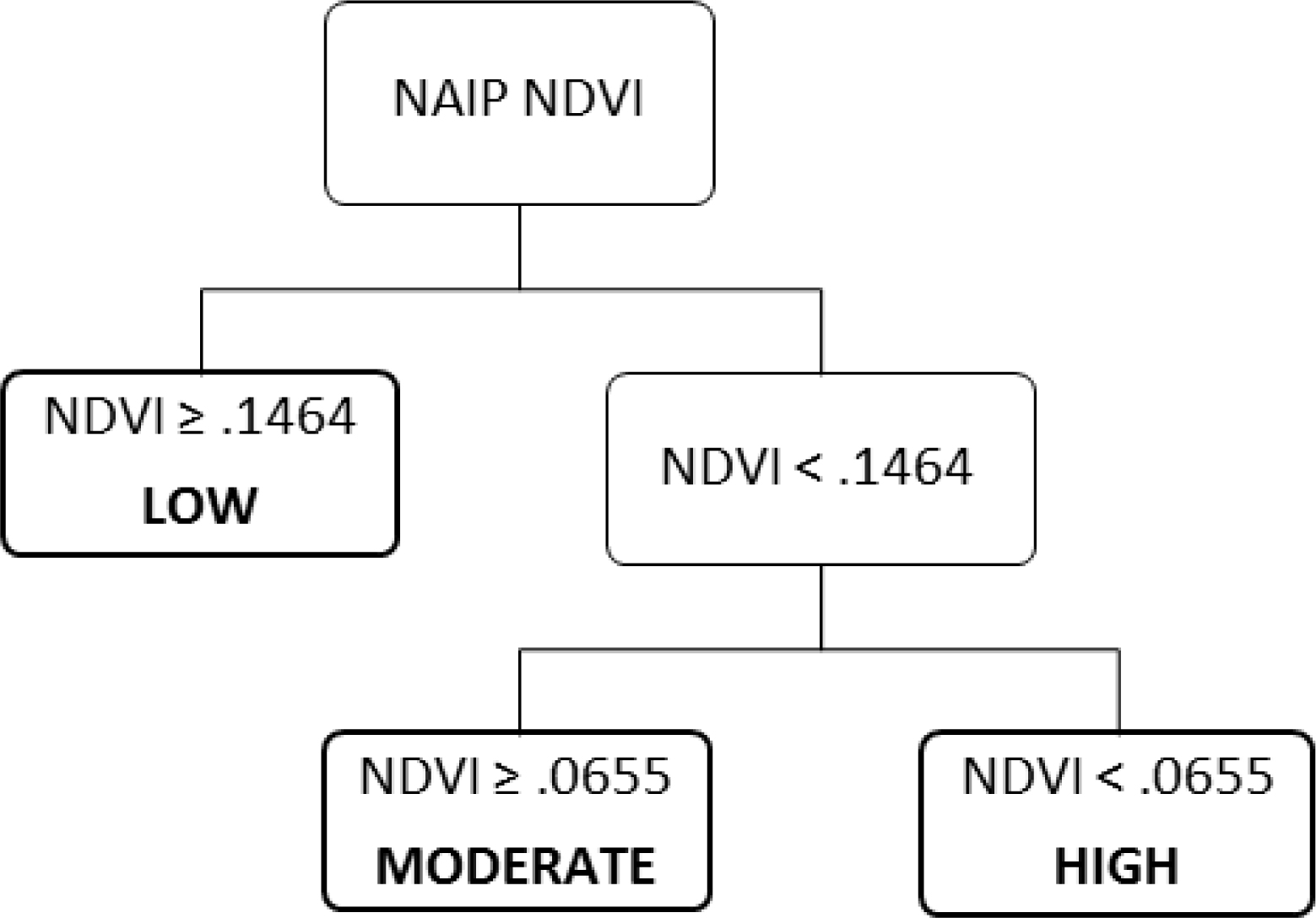
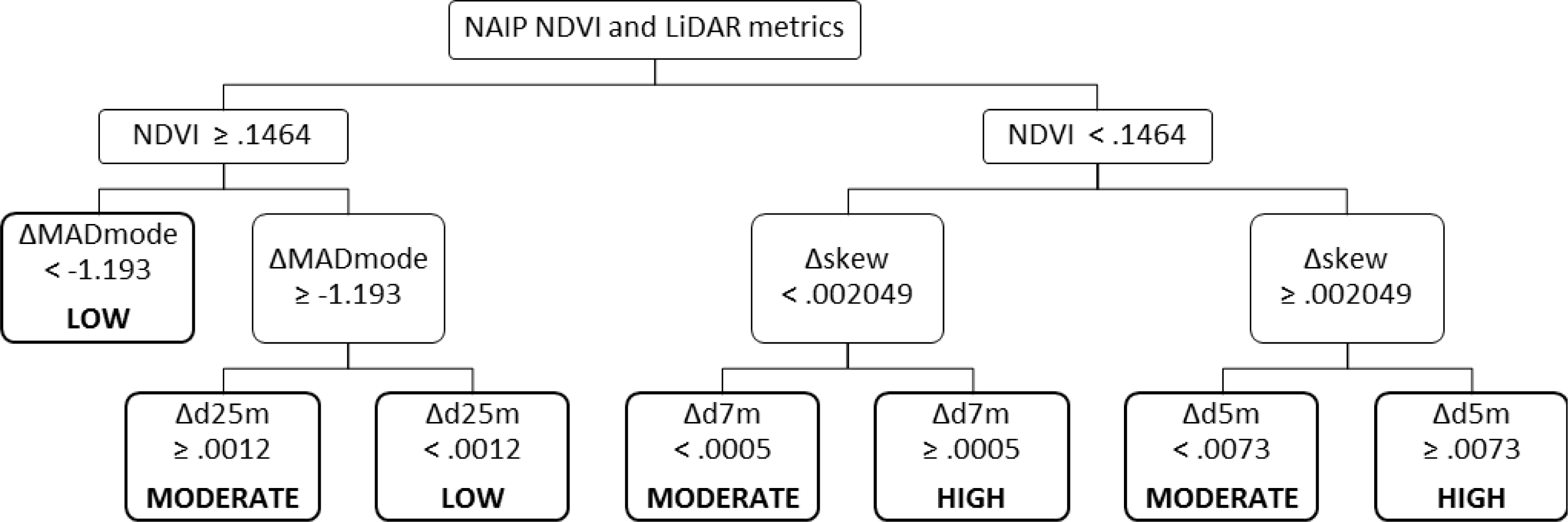
In this study, we combined NDVI from NAIP 1 m CIR imagery with a variety of metrics from pre- and post-fire LiDAR data to estimate the level of mortality of trees of all species at a plot scale, roughly equivalent to 0.08 ha (1/5 ac) plots. Three levels of mortality were defined based on plot percent mortality of trees 25.4 cm (10′′) DBH and greater. Estimates made using a Classification Analysis and Regression Tree (CART) approach with NDVI alone were compared to estimates made using NDVI in combination with post-fire only and with differenced pre- and post-fire LiDAR to assess whether gains in accuracy would result from the addition of LiDAR data. We had two objectives: first, to determine the accuracy that could be obtained using imagery alone, and compare any gains in accuracy that could be made by adding LiDAR data, and second, to demonstrate generation of wall-to-wall mortality estimates using imagery and LiDAR data.

2. Materials and Methods

2.1. Study Site

The study was conducted on a portion of Swanton Pacific Ranch, a 1,320 ha educational and research facility, dedicated to remain a working ranch and forest, owned by the Cal Poly Corporation and managed by the College of Agriculture, Food, and Environmental Sciences at Cal Poly. The ranch is located on the west slope of the Santa Cruz Mountains on the Central Coast of California, approximately 19 km north of the city of Santa Cruz. Elevations across the site range from approximately 20 to 470 m. The topography is steep and rugged with slopes ranging from 0% to 85%. The site experiences a maritime-Mediterranean climate, with cool rainy winters and dry summers, moderated by coastal fog. Overstory forest canopy in the study area is dominated by second-growth coast redwood (Sequoia sempervirens (D. Don) Endl.) with a significant component of Douglas-fir (Pseudotsuga menziesii (Mirbel) Franco var menziesii), tanoak (Lithocarpus densiflorus (Hook & Arn.) Rehder) and coast live-oak (Quercus agrifolia (Née)). Riparian corridors are dominated by red alder (Alnus rubra (Bong.)) with bigleaf maple (Acer macrophyllum (Pursh)) and California bay (Umbellularia californica (Hook. & Arn.) Nutt.). With the exception of a small stand at the northernmost extent, the entire study site was clearcut in the early 20th century. Portions of the site were salvage logged following the Pine Mountain Fire in 1948. Approximately 127 ha, 41% of the site, was selectively harvested between 1989 and 2008, with some portions harvested twice within this period. As a result, the structure of the forest is variable across the site, with 1–3 age classes present. Basal area (BA) within the plots range from 4 to 202 m²/ha; BA within plots used for this project range from 35 to 124 m²/ha. On 12 August 2009, a fire was ignited to the north of Swanton Pacific Ranch which would come to be known as the Lockheed Fire, and burn 3,163 ha over the course of 11 days. The entire site is located within the perimeter of the Lockheed fire, and experienced varying intensity and subsequent tree mortality. As a result of the fire, 37.5 hectares of the study area were salvage-logged using a helicopter in the winter of 2009 (see Figure 1b).

2.2. Tree Measurements

This study made use of 47 pre-existing 0.08 ha (1/5 acre) continuous forest inventory (CFI) plots, last inventoried either in 2003 or 2008. The plots are located on a 152.4 m (500′) systematic grid; plot locations were originally established using a staff compass and cloth tape. A variety of standard forest inventory data is collected every ten years at each CFI plot for every tree greater than 2.54 cm (1′′) DBH, however, data used in this analysis was limited to tree species, DBH, and tree status (live or dead). Tree status was assessed each year following the fire, through 2012, with the most recent status (2012) being used for this analysis. The diameters of trees in plots measured in 2003 was projected to 2008 using a growth rate of 2% [17]. The plot mortality used is the percent mortality in trees at least 25.4 cm (10′′) DBH, to avoid the confounding effect of the presence or absence, before the fire, of a large number of small trees in a plot; the 47 plots used are the subset of a total of 83 plots in the study area which have at least 15 trees which are at least 25.4 cm DBH. The diameter cutoff was chosen based on the professional experience of the authors; several cutoffs were informally tested, and the 25.4 cm value chosen as the most appropriate. Plot mortality of trees 25.4 cm (10′′) DBH and greater was coded as a categorical variable to determine the relative effectiveness of using only imagery, using imagery and post-fire LiDAR, and using imagery and pre- and post-fire LiDAR to classify mortality. The categories used and number of plots in each category are shown in

Table 1. Plot-level mortality categories.

Mortality of Trees 25.4 cm DBH and Greater (%)	Mortality Class	Number of Plots
<25	Low	20
25–50	Moderate	16
>50	High	11

.

These categories were chosen to provide enough information to land managers with as few classes as possible. In areas with less than 25% mortality of trees 25.4 cm DBH and greater, salvage harvesting is not likely to be economically viable, and the productivity of these areas is probably not significantly impacted by that level of mortality. In areas with greater than 50% mortality, harvesting is probably necessary to maintain productivity, and is very likely to be supported from an economic point of view. Areas in between will likely need further assessment based on the age, size, and density of timber, accessibility, and landowner objectives.

Plot center locations were collected during post-fire mortality assessment in 2009 using a Garmin 60csx GPS.

2.3. Imagery

National Agricultural Imagery Program (NAIP) 1 m CIR orthoimages taken in the summer of 2010 were downloaded as digital ortho-quarter-quads and stitched together in ESRI ArcMap 10.1. The spatial accuracy of the image was checked against two points which had been surveyed using conventional methods and which could be easily identified in the image; the average error was 2.54 m. The image has extensive deep shadows, which, in preliminary exploration of the data, interfered with the relationship between NDVI and mortality. The raw values of shadowed pixels were transformed using the following technique: an unsupervised classification process was used in ArcMap 10.1, with 7 classes, 2 of which corresponded with shadowed pixels. The resulting raster was reclassified to a set of binary masks representing either unshadowed or shadowed areas. These masks were used to extract samples of unshadowed and shadowed pixels from an unburned portion of the scene with similar vegetation as the fire area. Approximately 20 million unshadowed pixels and approximately 8 million shadowed pixels were compared. The distributions of pixel values from the sample are shown below in Figure 2.

The mean values of each sample of pixels were calculated. For band 1, the mean value of shadowed pixels was 73, while the mean value for unshadowed pixels was 135. For band 4, the mean value of shadowed pixels was 101, while the mean value for unshadowed pixels was 177. The values of shadowed pixels were adjusted by the difference in means (62 for band 1, and 76 for band 4). The resulting distributions, shown in Figure 3, are very similar. A similar technique was used by Sarabandi et al. [18] (2004) to correct shadowed pixels in IKONOS and QuickBird satellite imagery, although their correction also accounted for both differences in mean and standard deviation.

These adjusted bands were used to calculate NDVI. In order to isolate areas of forest cover versus grasses, shrubs and lower vegetation, the calculated NDVI raster was masked using a LiDAR-derived canopy height threshold of 2 m. The resulting NAIP adjusted NDVI for vegetation above 2 m in height is the NDVI used in all further analysis.

Initial, exploratory analysis of image NDVI and percent mortality was conducted using linear regression (not the coded mortality discussed above). The relationship between NDVI and mortality was determined to be different for shadowed versus unshadowed pixels, and the values of shadowed pixels were adjusted. As shown in Figure 4, adjustment yielded similar results as merely cropping out shadowed pixels. The benefit lies mainly in being able to use the entire scene, rather than having gaps, and in not basing some plots’ measurement on a very small number of pixels.

As mentioned in Section 2.3, the adjusted NDVI values were retained for areas where the LiDAR canopy height was greater than 2 m from the DEM. In fact, canopy-height masks at 1–5 m were tested, again using linear regression of plot percent mortality. The results, shown in

Table 2. Plot percent mortality on plot average NDVI masked from 0 to 5 m.

Average NDVI	R2
Whole plot	0.487
Above 1 m	0.513
Above 2 m	0.516
Above 3 m	0.521
Above 4 m	0.523
Above 5 m	0.524

, indicate that a higher threshold value might have yielded a better prediction; however, the number of pixels which contributed to the average values for some plots became small. The value of 2 m kept the proportion of all plots contributing above 60%, matched the threshold used for the LiDAR metrics, and still provided an improvement compared to unmasked data.

2.4. LiDAR

Two LiDAR data sets were used for this project: one collected 28–29 February 2008, and one 9–10 March 2010, both by Airborne1 corporation, El Segundo CA. The 2008 flight used an Optech ALTM 3100 sensor aboard a Cessna 210 fixed-wing aircraft, scanning at 100,000 Hz with a scan angle of 14°. The 2010 flight used an Optech ALTM Orion sensor aboard a Navajo Chieftain fixed-wing aircraft, scanning at 150,000 Hz with a scan angle of 14°. For both flights, 1-sigma horizontal accuracy was 30 cm, and vertical accuracy 18.3 cm at 95% confidence and 15.2 cm at 90% confidence, according to the vendor. Quality assurance for elevations was provided by the vendor using real-time kinematic GPS points. For the 2008 flight, 1,046 points were collected; RMSE for the LiDAR DEM was 0.03 m, with residuals ranging from −0.15 to 0.07 m. For the 2010 flight, 2,742 points were collected; RMSE for the DEM was 0.034 m, with residuals ranging from −0.052 to 0.03 m. Raw data from both flights were delivered in LAS format, filtered by the vendor to identify bare-earth ground returns, and with points classified as first, last, or intermediate returns. Average first-return density across the study area was 5.78 returns m² for the 2008 data and 8.12 returns m² for the 2010 data. The raw LiDAR data were clipped to the locations of the CFI plots and exported as comma-separated value files using FUSION LTK 3.30, developed by the US Forest Service. Height percentiles and a variety of other metrics describing the vertical distribution of LiDAR returns above 2 m, as suggested by White et al. (2013) in their best-practices guide, were calculated for each plot using the CloudMetrics tool in FUSION [19]. The number of points in 1 m height bins was calculated for each plot using the DensityMetrics tools in FUSION. Height percentiles were normalized by mean and mode, and point counts in 1 m height bins were normalized by total number of points, in Microsoft Excel. All metrics calculated were also differenced by subtracting 2008 values from 2010 values in Microsoft Excel.

3. Results

In order to provide a baseline for comparison, plot average, adjusted NDVI above 2 m was used to predict coded plot percent mortality (1–3) using a CART procedure. The confusion matrix for this prediction is shown in

Table 3. Confusion matrix, model A (NDVI).

	Classification				Omission
Reference	<25%	25%–50%	>50%	Total	error
<25%	19	1	0	20	0.05
25%–50%	6	10	1	17	0.41
>50%	0	4	6	10	0.40
Total	25	15	7	47
Commission error	0.24	0.33	0.14		0.26

; overall accuracy was 74%.

This model, shown in Figure 5, will be referred to as “model A”; a map of predicted mortality for the entire fire area based on this model can be found in Section 3.1.

Imagery and LiDAR

Plot mortality was classified using the combination of NDVI and post-fire LiDAR, and NDVI combined with pre- and post-fire LiDAR (differenced LiDAR). Again, a CART procedure was used, using leave-one-out cross-validation for variable selection. The CART procedure makes a series of splits in the data, selecting a variable to split the data into two classes at each step, such that the resulting classes are more homogenous than the parent. Using only post-fire LiDAR, the best model (model B) used:

• - NAIP 2010 adjusted NDVI above 2 m (NDVI);
• - 50th percentile/mean height of points above 2 m (p50/mean);
• - 50th percentile/mode height of points above 2 m (p50/mode);
• - Standard deviation of height of points above 2 m (St. Dev.);
• - Percent of points in the 16–17 m height bin (d17m).

The confusion matrix for model B is shown in

Table 4. Confusion matrix, model B (NDVI & post-fire LiDAR).

	Classification				Omission
Reference	<25%	25%–50%	>50%	Total	error
< 25%	17	2	1	20	0.15
25%–50%	1	15	1	17	0.12
>50%	0	2	8	10	0.20
Total	18	19	10	47
Commission error	0.06	0.21	0.20		0.15

, overall accuracy was 85%. The classification tree for the model is shown in Figure 6; a map of predicted mortality using this model can be found below.

Using differenced LiDAR, the best model (model C) included:

• - NAIP 2010 adjusted NDVI above 2 m (NDVI);
• - Change in skewness of height of points above 2 m (Δskew);
• - Change in median of absolute deviations from mode of height of points above 2 m (ΔMADmode);
• - Change in percent of points in the 4–5 m height bin (Δd5m);
• - Change in percent of points in the 6–7 m height bin (Δd7m);
• - Change in percent of points in the 24–25 m height bin (Δd25m).

The confusion matrix for model C is shown in

Table 5. Confusion matrix, model C (NDVI & differenced LiDAR).

	Classification				Omission
Reference	<25%	25%–50%	>50%	Total	error
<25%	18	2	0	20	0.10
25%–50%	1	16	0	17	0.06
>50%	0	5	5	10	0.50
Total	19	23	5	47
Commission error	0.05	0.30	0.00		0.17

; overall accuracy was 83%. The classification tree for the model is shown in Figure 7; a map of predicted mortality using this model can be found in Figure 8c.

Maps of estimated mortality were generated for the entire fire area using each of the methods above. These maps, shown in Figure 8, have a 30 m pixel size, chosen as an even number of meters that closely corresponds with the field plot size (900 compared to 809 m²). Because the pre-fire LiDAR data was collected for another project, it does not cover the entire fire area, although it covers the entire study area—thus the small area in the southeast portion of the fire area with no predicted mortality in Figure 8c. The remaining area with no predicted mortality in all three maps is the area where the LiDAR canopy height is within 2 m of the DEM.

4. Discussion

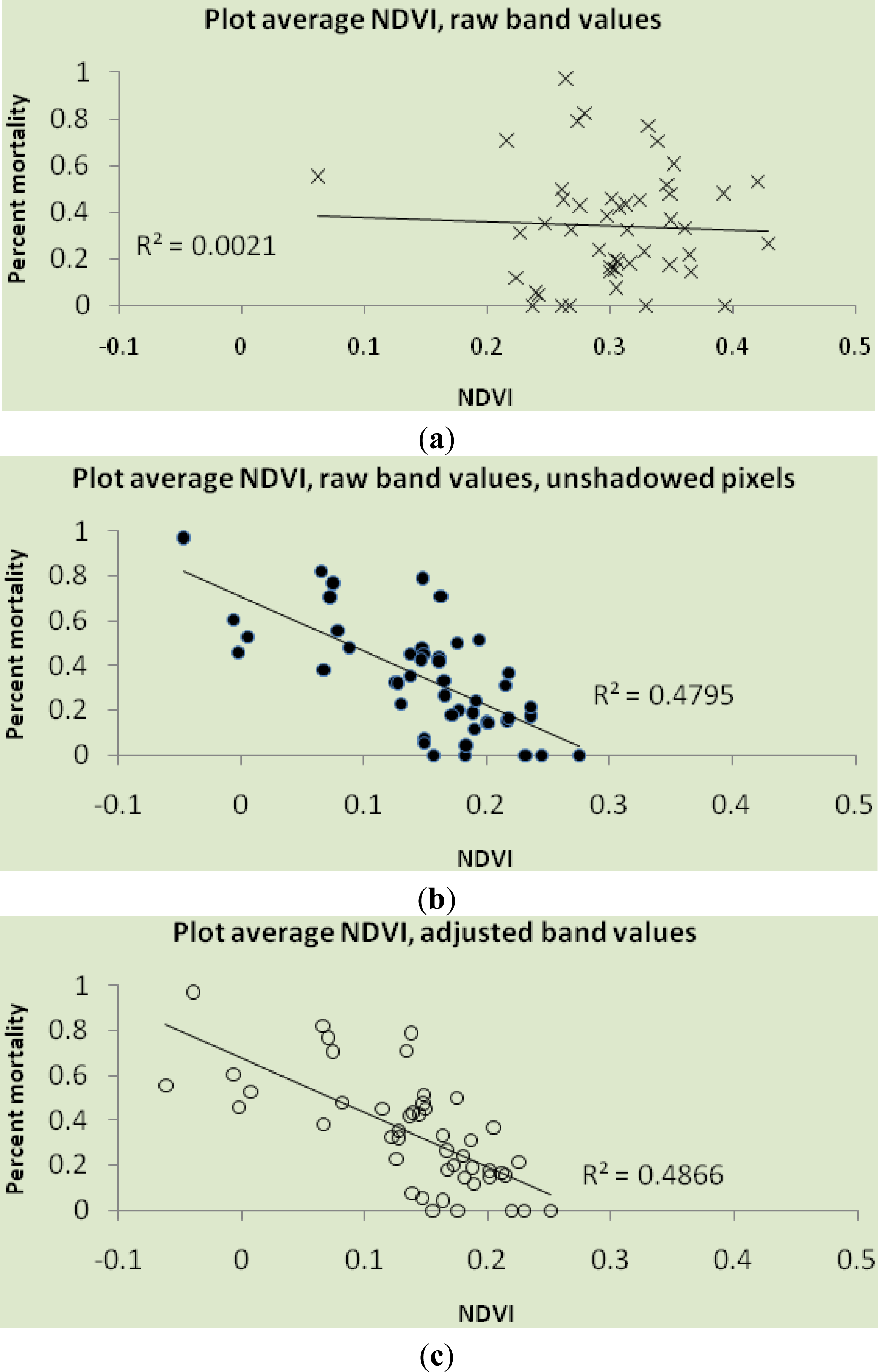
We presented a comparison of the accuracy of imagery-only, imagery fused with post-fire LiDAR, and imagery fused with differenced (pre- and post-fire) LiDAR in estimating plot-level mortality resulting from a wildfire in a typical second-growth coast redwood forest. We presented the percent accuracy of each method across 47 field plots. Using a single, freely available post-fire image (model A), mortality classes were estimated with 74% accuracy. Our results are similar to other studies which have used NDVI to estimate severity, although it is difficult to compare severity to mortality [3–5]. 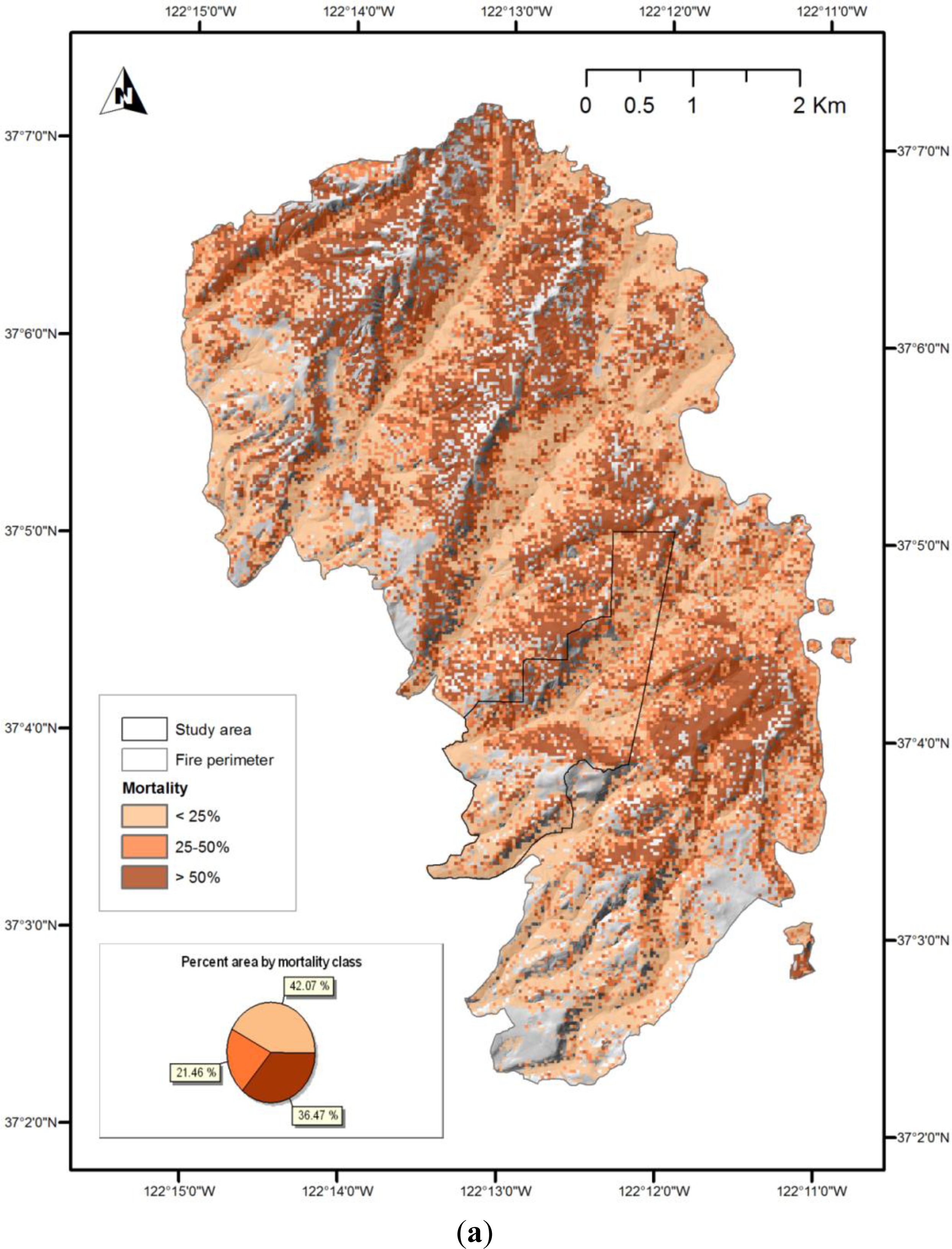Although approximately 40% of plots in the higher two mortality classes were misclassified, importantly, no plots with high mortality (>50%) were classified as low mortality (<25%), or vice-versa. In addition, we generated maps of estimated mortality across the entire fire area, for demonstration purposes. These maps should not be considered accurate, as the models they use are based on a limited sample, which does not represent all the forest types present across the fire area. However, they are likely to be as accurate in areas of similar forest type outside the study area as they are within it. Examination of the map of the model A prediction for the entire fire area, shown in Figure 8a, suggests that too much area was classified as low-mortality by this method; the confusion matrix suggests that some of this area should have been classified as moderate.

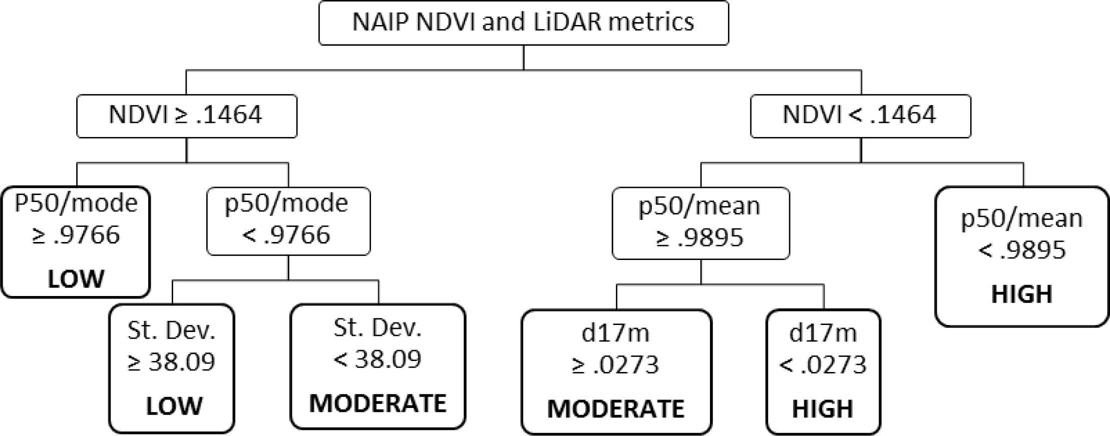
The combination of imagery with post-fire LiDAR data improved overall accuracy from 74% to 85%, compared to imagery alone. Most of the improvement can be attributed to plots which were incorrectly classified as low-mortality and which are in fact moderate-mortality. On the other hand, classification using post-fire LiDAR is less accurate when it comes to low-mortality plots, and classifies one of these plots as high-mortality, which is one of only two plots which were misclassified across two classes—the other being in the unshadowed NDVI classification.

Two of the LiDAR variables selected, the p50/mean and p50/mode, describe the skew in the data. The standard deviation is used in combination with p50/mode—where both are low, mortality is higher. Where both values are higher, there are a greater number of returns higher in the canopy, which presumably corresponds with greater vegetative structure, and lower mortality. Similarly, where the ratio of p50/mean is low, mortality is high, as it is where p50/mean is higher but the percentage of returns from 16 to 17 m is low. To state this another way, for similar values of NDVI, mortality is lower where p50/mean and d17 are high—where there are more returns higher in the canopy, by two different measures.

The addition of LiDAR data for post fire assessment is associated with substantial additional cost, though the data may be gathered for other purposes such as watershed or other risk assessments. At present, the question for land managers considering the use of LiDAR data for predicting mortality or characterizing fire severity will be whether this extra cost is justified by increased accuracy. As more uses are developed for the data, however, collection becomes more economically feasible. In addition, anecdotally, it appears that the extent of LiDAR acquisitions is increasing, and the future will likely bring more widely available, higher quality inexpensive or free LiDAR data.

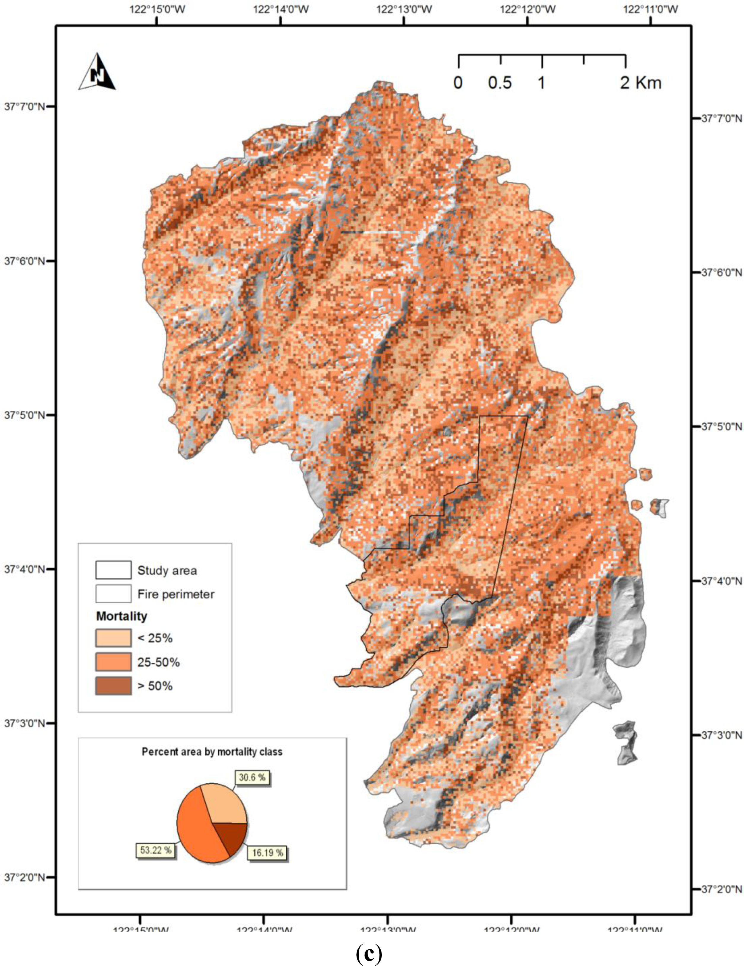
The combination of imagery with both pre- and post-fire LiDAR in a change-detection approach did not improve classification in this study. There was a slight decrease in overall accuracy compared to the post-fire LiDAR and imagery model, and this strategy yielded the lowest accuracy in the highest-mortality class of all strategies explored. Half of the plots with mortality greater than 50% were misclassified as moderate-mortality.

Similarly to model B, this model used variables describing the skew and variation in the data set—in this case, Δskew and ΔMADmode—and change in normalized densities in three height bins, from 4–5, 6–7, and 24–25 m. Where ΔMADmode was higher (positive or only slightly negative), and Δd25m was positive, mortality was higher, which seems counterintuitive—these characteristics indicate that LiDAR returns are more broadly distributed through the canopy, and that there is more structure high in the canopy. It may be, however, that this is only due to an absence of structure below 25 m. Where Δd7m and Δd5m were negative, mortality was lower, which seems reasonable if the change was due to more returns higher in the canopy, but this is not certain—it could also be due to a higher proportion of returns below those thresholds.

Unless pre- and post-fire data collections are made with differencing in mind, they will likely differ in density, which affects both DEM generation and canopy metrics in complex ways, interacting with slope and cover. These effects likely confound the relationships between metrics and actual aboveground structure, making relationships with mortality (or other attributes) difficult to detect. Similar problems were discovered by Kaufmann et al. [12]. It is possible that thinning the post-fire LiDAR point cloud to more closely match the pre-fire data would have provided better results. In addition, data sets may have been separated into files of manageable sizes using different grids, as was the case in this study. Differences in density and in gridding make calculation of differenced metrics much more complex and time-consuming than metrics from a single dataset. As a result, in most cases, differencing would have to yield a significant improvement in accuracy to justify the additional time and effort.

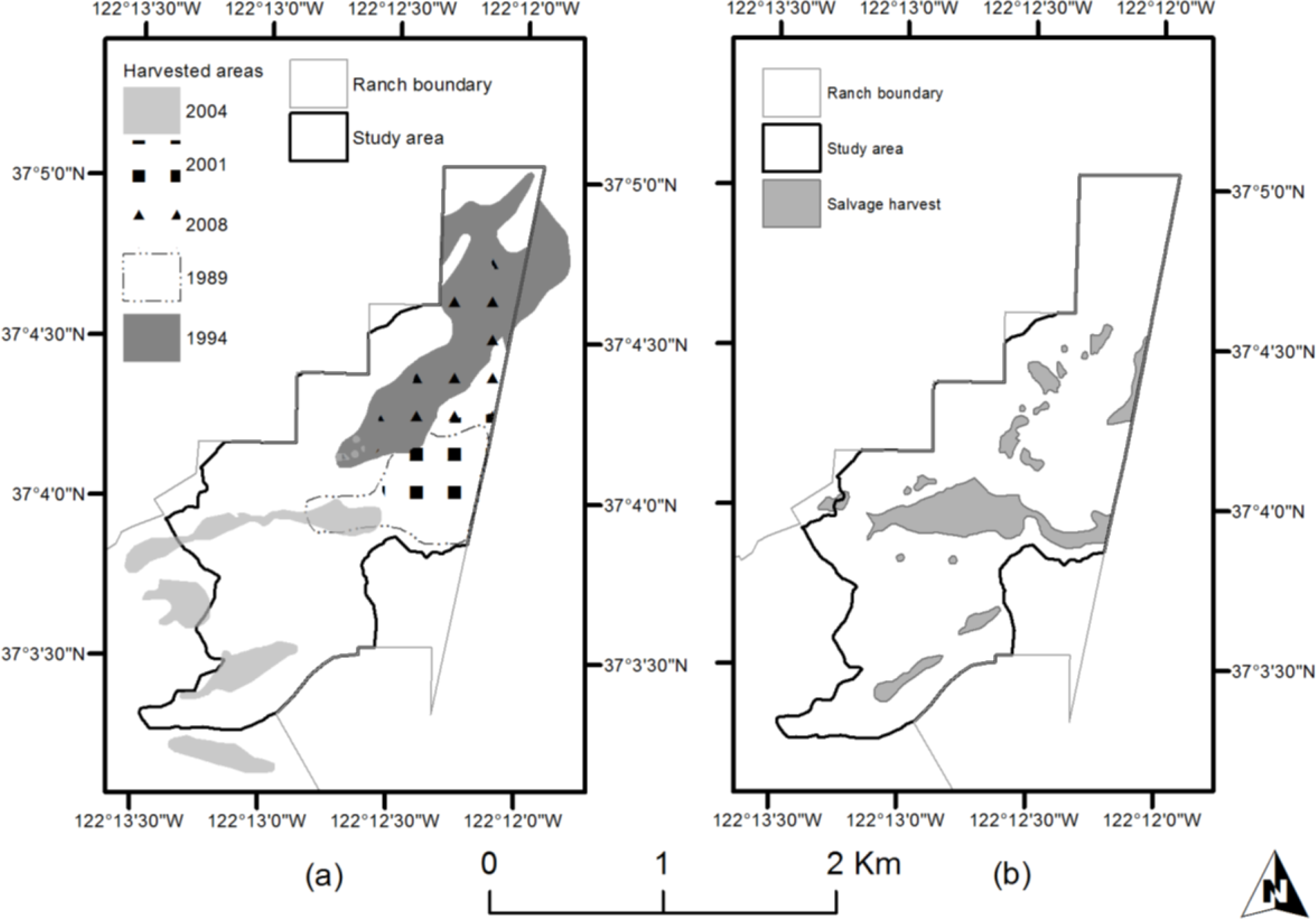
The Lockheed Fire began at the northern end of the fire area (shown in Figure 8) and was initially wind-driven, jumping from ridge to ridge in a south-east direction, and backing down to the drainages between. The fire was generally most intense on the ridge-tops, and least intense in drainages. All three methods used to map estimated mortality highlight a pattern which is generally consistent with this pattern of intensity, although model C (Figure 8c) shows only a weak pattern related to topography.

Field measurements used in this study are limited to diameter and status (live or dead). Field survey crews were trained in proper procedures, and mortality was assessed three separate times over three years [17]. However, it is possible that there are errors in the field data used.

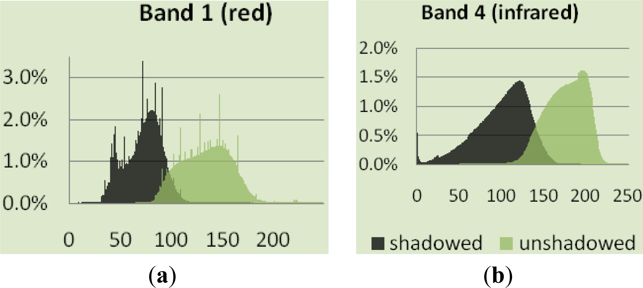
The LiDAR vendor for the data used in this study stated the vertical accuracy of the data was 18.3 cm at 95% confidence, and 15.2 cm at 90% confidence, and the 1σ horizontal accuracy as 30 cm. These accuracies are based on measurements made under better than average conditions across the study area. The accuracy is likely lower in areas with dense forest canopy, especially in the pre-fire data.

The field plots used in this study were originally established on a 152.4 m (500′) grid, based on a variety of control points, using a staff compass and cloth tape. Coordinate locations for these plots were collected with a Garmin 60 csx GPS, which is a consumer-grade unit. While their ultimate accuracy is lower than that of mapping-grade units, personal experience working in the study area has demonstrated that currently available mapping-grade units will not establish a position in many plot locations. Horizontal positional accuracy of these locations is estimated to be within 10–15 m, though an independent accuracy assessment has not been conducted. However, a similar unit, deployed in forested conditions, had average RMSE of 16.88 m, with the authors calculating 95th percentile RMSE to be 29.22 m [20]. Using these values, the average plot would have an error representing approximately 64% of the plot area—this is the proportion of the remote sensing data that is outside the field plot. The 95% error stated is nearly equal to the plot diameter—only 3% of the remote sensing data sampled would be from the actual area of the field plot. The consequences of errors in plot locations are probably less than might be suggested by the percentages stated, given that some area immediately outside plots will contain canopies of trees which are in fact located within those plots, while a similar area which is in fact part of the plot will contain canopies of trees which are outside the plot. In addition, the mortality of larger trees is not expected to be drastically different over the space of a few meters. In general, plots nearer to control points had locations closer to the original grid, while those further from control points appear to have more error, as would be expected if the actual locations of plots conform less to the grid as the distance from control increases, and the GPS points are more accurate.

5. Conclusions

This study demonstrates that remote sensing data can be used to estimate plot-level tree mortality resulting from wildfire with a modest degree of accuracy. The combination of imagery and post-fire LiDAR data yielded a moderate increase in overall accuracy compared to the use of imagery alone, while the combination of imagery and differenced LiDAR data yielded a small decrease in overall accuracy compared to the use of only post-fire LiDAR, though it still increased accuracy compared to imagery alone.

Further research is recommended to investigate the improvement in accuracy that can be made using post-fire LiDAR and imagery, and to determine whether thinning of the post-fire LiDAR point cloud to match the pre-fire density has any impact on results using differenced LiDAR.

The CART procedure used is a powerful tool for modelling a categorical response, which requires fewer assumptions than linear or logistic regression, and offers simpler interpretation of output. The approach and methods used in this study could be adapted to rapidly estimate the mortality of trees that is expected to result from wildfires, at scales that would not be practical or economical using field-based methods.

References

1. Key, C.H.; Benson, N.C. Landscape Assessment; US Forest Service: Fort Collins, CO, USA, 2006; p. 51. Available online: http://www.treesearch.fs.fed.us/pubs/24066 (accessed on 27 February 2014).
2. Coppin, P.; Jonckheere, I.; Nackaerts, K.; Muys, B.; Lambin, E. Digital change detection methods in ecosystem monitoring: A review. Int. J. Remote Sens 2004, 25, 1565–1596. [Google Scholar]
3. Epting, J.; Verbyla, D.; Sorbel, B. Evaluation of remotely sensed indices for assessing burn severity in interior Alaska using Landsat TM and ETM+. Remote Sens. Environ 2005, 96, 328–339. [Google Scholar]
4. Escuin, S.; Navarro, R.; Fernández, P. Fire severity assessment by using NBR (Normalized Burn Ratio) and NDVI (Normalized Difference Vegetation Index) derived from LANDSAT TM/ETM images. Int. J. Remote Sens 2008, 29, 1053–1073. [Google Scholar]
5. Rogan, J.; Yool, S.R. Mapping fire-induced vegetation depletion in the Peloncillo Mountains, Arizona and New Mexico. Int. J. Remote Sens 2001, 22, 3101–3121. [Google Scholar]
6. Kane, V.R.; Lutz, J.A.; Roberts, S.L.; Smith, D.F.; McGaughey, R.J.; Povak, N.A.; Brooks, M.L. Landscape-scale effects of fire severity on mixed-conifer and red fir forest structure in Yosemite National Park. For. Ecol. Manag 2013, 287, 17–31. [Google Scholar]
7. Goerndt, M.E.; Monleon, V.J.; Temesgen, H. Relating forest attributes with area- and tree-based light detection and ranging metrics for western Oregon. West. J. Appl. For 2010, 25, 105–111. [Google Scholar]
8. Falkowski, M.J.; Evans, J.S.; Martinuzzi, S.; Gessler, P.E.; Hudak, A.T. Characterizing forest succession with lidar data: An evaluation for the Inland Northwest, USA. Remote Sens. Environ 2009, 113, 946–956. [Google Scholar]
9. Hill, R.A.; Broughton, R.K. Mapping the understorey of deciduous woodland from leaf-on and leaf-off airborne LiDAR data: A case study in lowland Britain. ISPRS J. Photogramm. Remote Sens 2009, 64, 223–233. [Google Scholar]
10. Martinuzzi, S.; Vierling, L.A.; Gould, W.A.; Falkowski, M.J.; Evans, J.S.; Hudak, A.T.; Vierling, K.T. Mapping snags and understory shrubs for a LiDAR-based assessment of wildlife habitat suitability. Remote Sens. Environ 2009, 113, 2533–2546. [Google Scholar]
11. Kim, Y.; Yang, Z.Q.; Cohen, W.B.; Pflugmacher, D.; Lauver, C.L.; Vankat, J.L. Distinguishing between live and dead standing tree biomass on the North Rim of Grand Canyon National Park, USA using small-footprint lidar data. Remote Sens. Environ 2009, 113, 2499–2510. [Google Scholar]
12. Kaufmann, M.R.; Stoker, J.M.; Greenlee, S.K. Using Lidar to Identify Sediment and Forest Structure Change in the Hayman Burn, Colorado. Final Report, Joint Fire Sciences Program Project No. 03-2-3-18; Available online: http://www.firescience.gov/projects/03-2-3-18/project/03-2-3-18_final_report.pdf (accessed on 27 February 2014).
13. Angelo, J.J.; Duncan, B.W.; Weishampel, J.F. Using Lidar-derived vegetation profiles to predict time since fire in an Oak Scrub landscape in East-Central Florida. Remote Sens 2010, 2, 514–525. [Google Scholar]
14. Wang, C.; Glenn, N.F. Estimation of fire severity using pre- and post-fire LiDAR data in sagebrush steppe rangelands. Int. J. Wildland Fire 2009, 18, 848–856. [Google Scholar]
15. Jakubowksi, M.K.; Guo, Q.H.; Collins, B.; Stephens, S.; Kelly, M. Predicting surface fuel models and fuel metrics using Lidar and CIR imagery in a dense, mountainous forest. Photogramm. Eng. Remote Sens 2013, 79, 37–49. [Google Scholar]
16. Mutlu, M.; Popescu, S.C.; Stripling, C.; Spencer, T. Mapping surface fuel models using Lidar and multispectral data fusion for fire behavior. Remote Sens. Environ 2008, 112, 274–285. [Google Scholar]
17. Auten, S. Mortality Assessment of Redwood and Mixed Conifer Forest Types in Santa Cruz County Following Wildfire; California Polytechnic State University: San Luis Obispo, CA, USA, 2012. [Google Scholar]
18. Sarabandi, P.; Yamazaki, F.; Matsuoka, M. Shadow Detection and Radiometric Restoration in Satellite High Resolution Images. Proceedings of the 2004 IEEE International Geoscience and Remote Sensing Symposium, IGARSS’ 04, Anchorage, AK, USA, 20–24 September 2004; 6, pp. 3744–3747.
19. White, J.C.; Wulder, M.A.; Varhola, A.; Vastaranta, M.; Coops, N.C.; Cook, B.D.; Pitt, D.; Woods, M. A Best Practices Guide for Generating Forest Inventory Attributes from Airborne Laser Scanning Data Using an Area-Based Approach. Information Report FI-X-010;. Natural Resources Canada, Canadian Forest Service, Canadian Wood Fibre Centre: Victoria, BC, Canada, 2013. Available online: https://cfs.nrcan.gc.ca/publications?id=34887 (accessed on 27 February 2014).
20. Danskin, S.D.; Bettinger, P.; Jordan, T.R.; Cieszewski, C. A comparison of GPS performance in a southern Hardwood forest: Exploring low-cost solutions for forestry applications. South. J. Appl. For 2009, 33, 9–16. [Google Scholar]
Figure 1. Harvest history within the study area (a) regular commercial harvest; (b) salvage harvest in 2009.
Remotesensing 06 01954f1
Figure 2. Raw band values, unburned sample area, from (a) band 1 (red); (b) band 4 (infrared).
Remotesensing 06 01954f2
Figure 3. Adjusted band values, unburned sample area, from (a) band 1 (red); (b) band 4 (infrared).
Remotesensing 06 01954f3
Figure 4. Linear fit for plot percent mortality on NDVI for (a) all pixels; (b) only unshadowed pixels; (c) all pixels, shadowed pixels have been adjusted.
Remotesensing 06 01954f4
Figure 5. Classification tree for Model A, imagery only.
Remotesensing 06 01954f5
Figure 6. Classification tree for Model B, imagery and post-fire LiDAR.
Remotesensing 06 01954f6
Figure 7. Classification tree for Model C, imagery and differenced LiDAR.
Remotesensing 06 01954f7
Figure 8. Maps of estimated mortality for the entire fire area using (a) Model A—NDVI only; (b) Model B—NDVI & post-fire LiDAR; (c) Model C—NDVI & differenced LiDAR.
Remotesensing 06 01954f8aRemotesensing 06 01954f8bRemotesensing 06 01954f8c