Artificial Neural Network Modeling of High Arctic Phytomass Using Synthetic Aperture Radar and Multispectral Data

Abstract
:1. Introduction
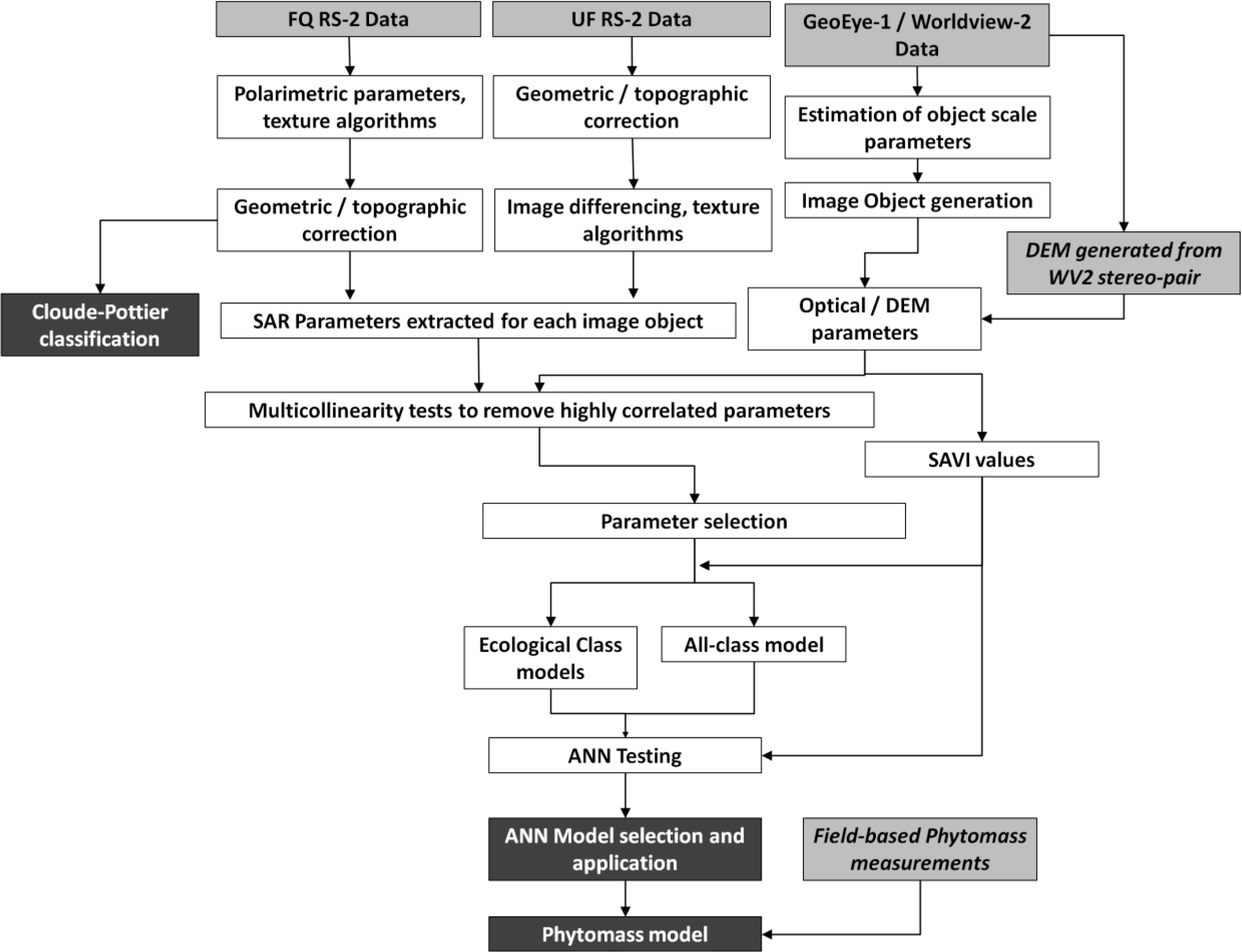
2. Methods
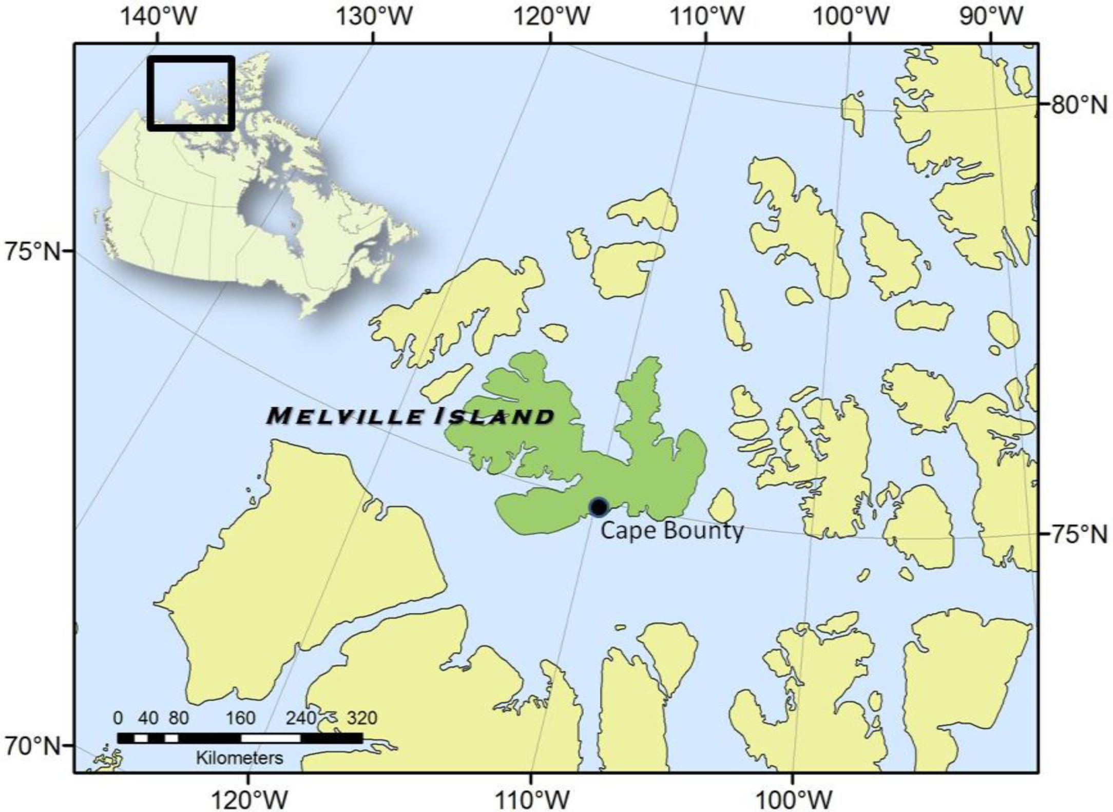
2.1. Study Location and Site Description
2.2. Optical Imagery
2.3. Object-Based Image Analysis (OBIA)
2.4. SAR Data
2.5. Vegetation Modeling
3. Results and Discussion
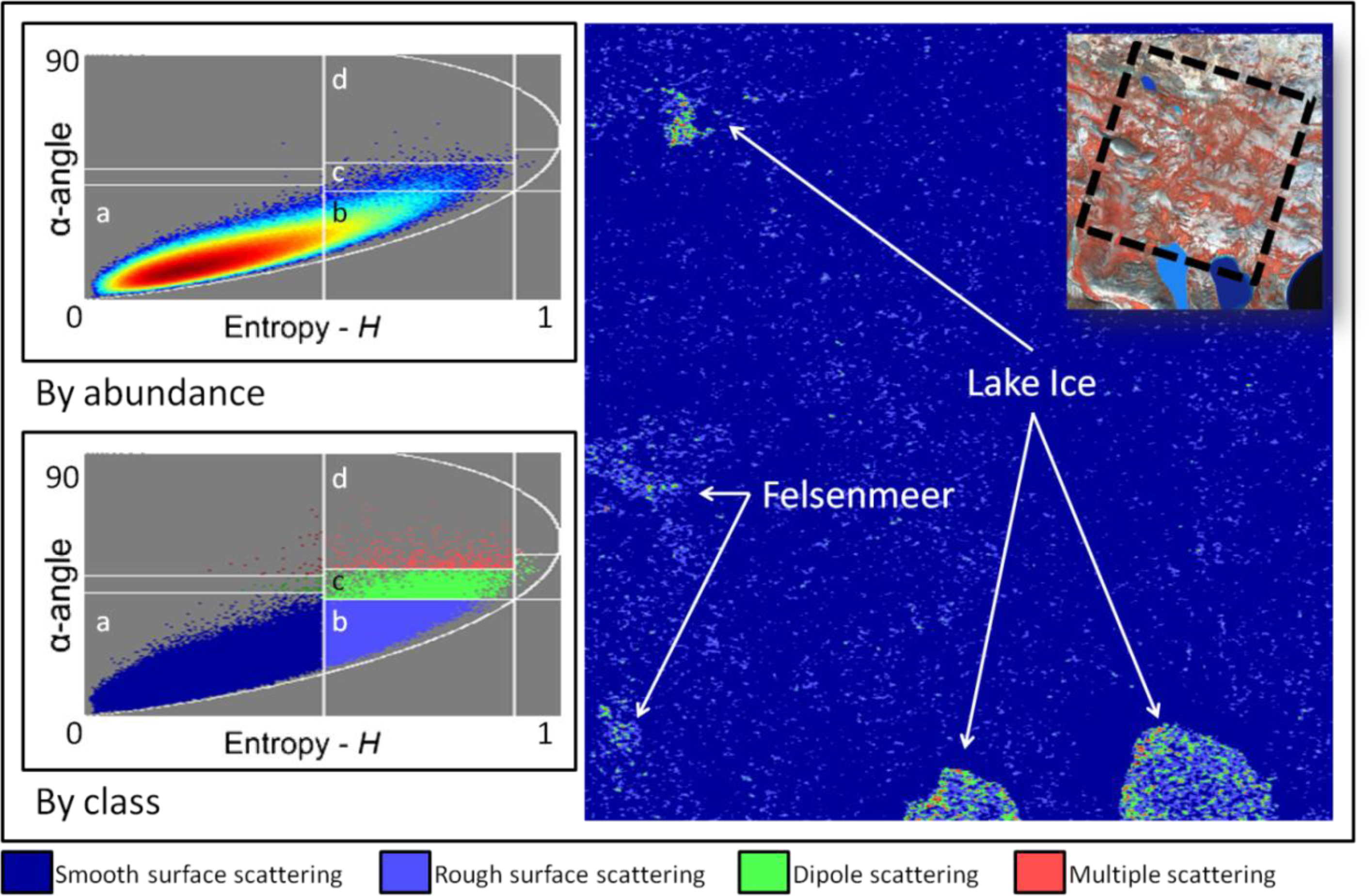
3.1. Scattering Mechanisms
3.2. ANN Models
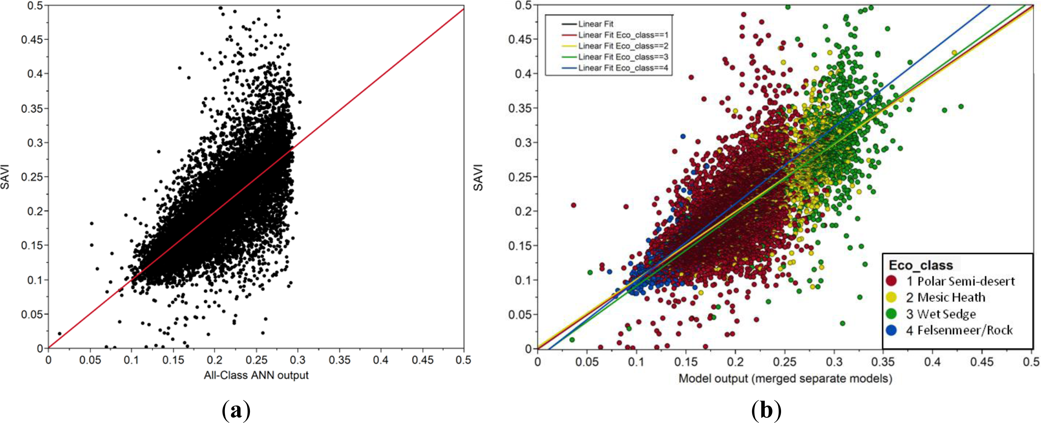
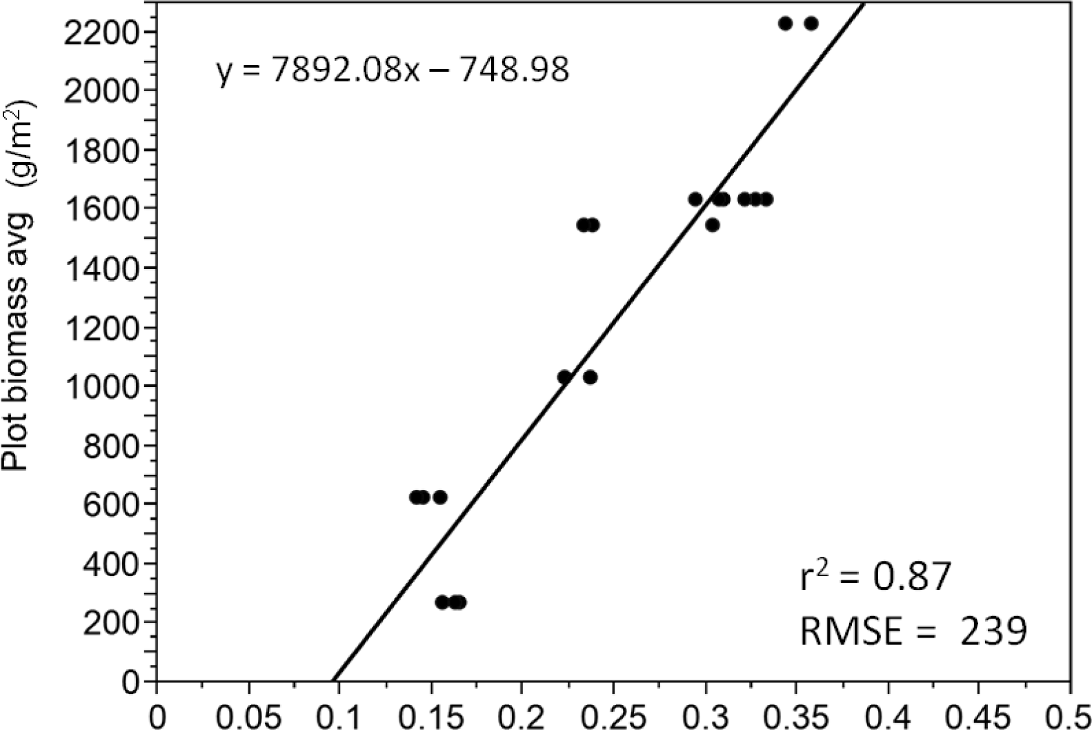
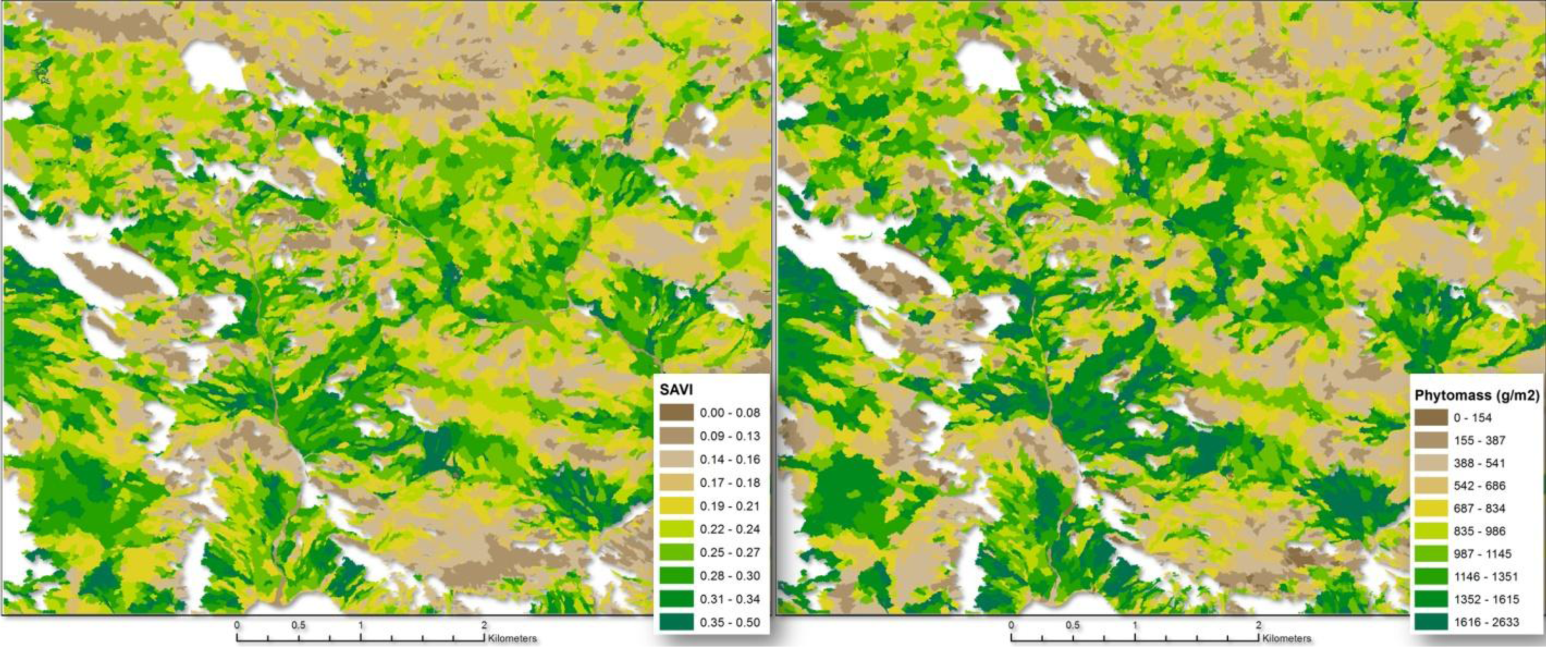
3.3. Above-Ground Phytomass Modeling
4. Conclusions
Acknowledgments
Author Contributions
Conflicts of Interest
References
- Walker, D.A.; Epstein, H.E.; Raynolds, M.K.; Kuss, P.; Kopecky, M.A.; Frost, G.V.; Daniëls, F.J.A.; Leibman, M.O.; Moskalenko, N.G.; Matyshak, G.V.; et al. Environment, vegetation and greenness (NDVI) along the North America and Eurasia Arctic transects. Environ. Res. Lett 2012, 7. [Google Scholar] [CrossRef]
- Raynolds, M.K.; Walker, D.A.; Maier, H.A. NDVI patterns and phytomass distribution in the circumpolar Arctic. Remote Sens. Environ 2006, 102, 271–281. [Google Scholar]
- Boelman, N.T.; Stieglitz, M.; Rueth, H.M.; Sommerkorn, M.; Griffin, K.L.; Shaver, G.R.; Gamon, J.A. Response of NDVI, biomass, and ecosystem gas exchange to long-term warming and fertilization in wet sedge tundra. Oecologia 2003, 135, 414–421. [Google Scholar]
- Shaver, G.R.; Street, L.E.; Rastetter, E.B.; van Wijk, M.T.; Williams, M. Functional convergence in regulation of net CO2 flux in heterogeneous tundra landscapes in Alaska and Sweden. J. Ecol 2007, 95, 802–817. [Google Scholar]
- Torn, M.S.; Chapin, F.S. Environmental and biotic controls over methane flux from arctic tundra. Chemosphere 1993, 26, 357–368. [Google Scholar]
- Parker, G.R.; Ross, R.K. Summer habitat use by muskoxen (ovibos moschatus) and peary caribou (rangifer tarandus pearyi) in the Canadian High Arctic. Polarforschung 1975, 1, 12–25. [Google Scholar]
- Abuelgasim, A.A.; Leblanc, S.G. Leaf area index mapping in northern Canada. Int. J. Remote Sens 2011, 32, 5059–5076. [Google Scholar]
- Laidler, G.J.; Treitz, P.M.; Atkinson, D.M. Remote sensing of arctic vegetation: Relations between the NDVI, spatial resolution and vegetation cover on boothia peninsula, nunavut. Arctic 2008, 61, 1–13. [Google Scholar]
- Atkinson, D.M.; Treitz, P. Modeling biophysical variables across an arctic latitudinal gradient using high spatial resolution remote sensing data. Arctic Antarct. Alp. Res 2013, 45, 161–178. [Google Scholar]
- Shaver, G.R.; Chapin, F.S.I. Response to fertilization by various plant growth forms in an alaskan tundra: nutrient accumulation and growth. Ecology 1980, 61, 662–675. [Google Scholar]
- Van Wijk, M.T.; Williams, M.; Shaver, G.R. Tight coupling between leaf area index and foliage N content in arctic plant communities. Oecologia 2005, 142, 421–427. [Google Scholar]
- Billings, W.D. Arctic and alpine vegetations: Similarities, differences, and susceptibility to disturbance. Bioscience 1973, 23, 697–704. [Google Scholar]
- Evans, B.M.; Walker, D.A.; Benson, C.S.; Nordstrand, E.A.; Petersen, G.W. Spatial interrelationships between terrain, snow distribution and vegetation patterns at an arctic foothills site in Alaska. Ecography 1989, 12, 270–278. [Google Scholar]
- Walker, D.A.; Kuss, P.; Epstein, H.E.; Kade, A.N.; Vonlanthen, C.M.; Raynolds, M.K.; Daniëls, F.J.A. Vegetation of zonal patterned-ground ecosystems along the North America Arctic bioclimate gradient. Appl. Veg. Sci 2011, 14, 440–463. [Google Scholar]
- Sitch, S.; McGuire, A.D.; Kimball, J.; Gedney, N.; Gamon, J.; Engstrom, R.; Wolf, A.; Zhuang, Q.; Clein, J.; McDonald, K.C. Assessing the carbon balance of circumpolar Arctic tundra using remote sensing and process modeling. Ecol. Appl 2007, 17, 213–234. [Google Scholar]
- Williams, M.; Bell, R.; Spadavecchia, L.; Street, L.E.; van Wijk, M.T. Upscaling leaf area index in an Arctic landscape through multiscale observations. Glob. Chang. Biol 2008, 14, 1517–1530. [Google Scholar]
- Loranty, M.M.; Goetz, S.J.; Rastetter, E.B.; Rocha, A.V; Shaver, G.R.; Humphreys, E.R.; Lafleur, P.M. Scaling an instantaneous model of tundra nee to the arctic landscape. Ecosystems 2011, 14, 76–93. [Google Scholar]
- Barrett, B.W.; Dwyer, E.; Whelan, P. Soil moisture retrieval from active spaceborne microwave observations: An evaluation of current techniques. Remote Sens 2009, 1, 210–242. [Google Scholar]
- Bindlish, R.; Barros, A.P. Parameterization of vegetation backscatter in radar-based, soil moisture estimation. Remote Sens. Environ 2001, 76, 130–137. [Google Scholar]
- Trudel, M.; Charbonneau, F.; Leconte, R. Using RADARSAT-2 polarimetric and ENVISAT-ASAR dual-polarization data for estimating soil moisture over agricultural fields. Can. J. Remote Sens 2012, 38, 1–14. [Google Scholar]
- Paloscia, S.A. Summary of experimental results to assess the contribution of SAR for mapping vegetation biomass and soil moisture. Can. J. Remote Sens 2002, 28, 246–261. [Google Scholar]
- Mattia, F.; Le Toan, T.; Picard, G.; Posa, F.I.; D’Alessio, A.; Notarnicola, C.; Gatti, A.M.; Rinaldi, M.; Satalino, G.; Pasquariello, G. Multitemporal C-band radar measurements on wheat fields. IEEE Trans. Geosci. Remote Sens 2003, 41, 1551–1560. [Google Scholar]
- Morrissey, L.A.; Livingston, G.P.; Durden, S.L. Use of SAR in regional methane exchange studies. Int. J. Remote Sens 1994, 15, 1337–1342. [Google Scholar]
- Moran, M.S.; Peters-Lidard, C.D.; Watts, J.M.; McElroy, S. Estimating soil moisture at the watershed scale with satellite-based radar and land surface models. Can. J. Remote Sens 2004, 30, 805–826. [Google Scholar]
- McNairn, H.; Hochheim, K.; Rabe, N. Applying polarimetric radar imagery for mapping the productivity of wheat crops. Can. J. Remote Sens 2004, 30, 517–524. [Google Scholar]
- Smith, A.M.; Buckley, J.R. Investigating RADARSAT-2 as a tool for monitoring grassland in western Canada. Can. J. Remote Sens 2011, 37, 93–102. [Google Scholar]
- Ulaby, F.T.; Moore, R.K.; Fung, K.A. Microwave Remote Sensing: Active and Passive. In Theory to Applications; Artech House, Inc.: Dedham, MA, USA, 1986; Volume 3. [Google Scholar]
- Kim, Y.; van Zyl, J.J.A. Time-series approach to estimate soil moisture using polarimetric radar data. IEEE Trans. Geosci. Remote Sens 2009, 47, 2519–2527. [Google Scholar]
- Moran, M.S.; Hymer, D.C.; Qi, J.; Sano, E.E. Soil moisture evaluation using multi-temporal synthetic aperture radar (SAR) in semiarid rangeland. Agric. For. Meteorol 2000, 105, 69–80. [Google Scholar]
- Sano, E.E.; Huete, A.R.; Troufleau, D.; Moran, M.S.; Vidal, A. Relation between ERS-1 synthetic aperture radar data and measurements of surface roughness and moisture content of rocky soils in a semiarid rangeland. Water Resour. Res 1998, 34, 1491–1498. [Google Scholar]
- Gross, M.F.; Hardisky, M.A.; Doolittle, J.A.; Klemas, V. Relationships among depth to frozen soil, soil wetness, and vegetation type and biomass in Tundra near Bethel, AK, USA. Arct. Alp. Res 1990, 22, 275–282. [Google Scholar]
- Meade, N.G.; Hinzman, L.D.; Kane, D.L. Spatial estimation of soil moisture using synthetic aperture radar in Alaska. Adv. Sp. Res 1999, 24, 935–940. [Google Scholar]
- Sahebi, M.R.; Bonn, F.; Bénié, G.B. Neural networks for the inversion of soil surface parameters from synthetic aperture radar satellite data. Can. J. Civ. Eng 2004, 31, 95–108. [Google Scholar]
- Said, S.; Kothyari, U.C.; Arora, M.K. ANN-Based soil moisture retrieval over bare and vegetated areas using ERS-2 SAR data. J. Hydrol. Eng 2008, 13, 461–475. [Google Scholar]
- Del Frate, F.; Wang, L. Sunflower biomass estimation using a scattering model and a neural network algorithm. Int. J. Remote Sens 2001, 22, 1235–1244. [Google Scholar]
- Mas, J.F.; Flores, J.J. The application of artificial neural networks to the analysis of remotely sensed data. Int. J. Remote Sens 2008, 29, 617–663. [Google Scholar]
- Raynolds, M.K.; Walker, D.A.; Epstein, H.E.; Pinzon, J.E.; Tucker, C.J.A. New estimate of tundra-biome phytomass from trans-Arctic field data and AVHRR NDVI. Remote Sens. Lett 2012, 3, 403–411. [Google Scholar]
- Gregory, F.M. Biophysical Remote Sensing and Terrestrial CO2 Exchange at Cape Bounty, Melville Island; Queen’s University: Kingston, ON, Canada, 2011; p. 161. [Google Scholar]
- Tenhunen, J.D.; Lange, O.L.; Hahn, S.; Siegwolf, R.; Oberbauer, S.F. The Ecosystem Role of Poikilohydric Tundra Plants. In Arctic Ecosystems in a Changing Climate; Chapin, F.S.I., Jefferies, R.L., Reynolds, J.F., Shaver, G.R., Svoboda, J., Eds.; Academic Press: San Diego, CA, USA, 1992; pp. 213–237. [Google Scholar]
- Douma, J.C.; van Wijk, M.T.; Lang, S.I.; Shaver, G.R. The contribution of mosses to the carbon and water exchange of arctic ecosystems: Quantification and relationships with system properties. Plant. Cell Environ 2007, 30, 1205–1215. [Google Scholar]
- Harris, A. Spectral reflectance and photosynthetic properties of sphagnum mosses exposed to progressive drought. Ecohydrology 2008, 1, 35–42. [Google Scholar]
- Bubier, J.L.; Rock, B.N.; Crill, P.M. Spectral reflectance measurements of boreal wetland and forest mosses. J. Geophys. Res 1997, 102, 29483–29494. [Google Scholar]
- Watanabe, M.; Kadosaki, G.; Kim, Y.; Ishikawa, M.; Kushida, K.; Sawada, Y.; Tadono, T.; Fukuda, M.; Sato, M. Analysis of the sources of variation in L-band backscatter from terrains with permafrost. IEEE Trans. Geosci. Remote Sens 2012, 50, 44–54. [Google Scholar]
- Huete, A.R. A soil-adjusted vegetation index (SAVI). Remote Sens. Environ 1988, 25, 295–309. [Google Scholar]
- Atkinson, D.M.; Treitz, P. Arctic ecological classifications derived from vegetation community and satellite spectral data. Remote Sens 2012, 4, 3948–3971. [Google Scholar]
- Hodgson, D.A.; Vincent, J.-S. A 10,000 yr B.P. extensive ice shelf over viscount melville sound, arctic Canada. Quat. Res 1984, 22, 18–30. [Google Scholar]
- Lajeunesse, P.; Hanson, M.A. Field observations of recent transgression on northern and eastern Melville Island, western Canadian Arctic Archipelago. Geomorphology 2008, 101, 618–630. [Google Scholar]
- CAVM Team. Circumpolar Arctic Vegetation Map, scale 1: 7,500,000; Conservation of Arctic Flora and Fauna (CAFF) Map No. 1; CAVM Team: Anchorage, AK, USA, 2003. [Google Scholar]
- Guisan, A.; Weiss, S.B.; Weiss, A.D. GLM versus CCA spatial modeling of plant species distribution. Plant Ecol 1999, 143, 107–122. [Google Scholar]
- Jenness, J.; Brost, B.; Beier, P. Land Facet Corridor Designer: Extension for ArcGIS. Available online: http://www.jennessent.com/arcgis/land_facets.htm (accessed on 7 March 2014).
- Blaschke, T. Object based image analysis for remote sensing. ISPRS J. Photogramm. Remote Sens 2010, 65, 2–16. [Google Scholar]
- Drăguţ, L.; Schauppenlehner, T.; Muhar, A.; Strobl, J.; Blaschke, T. Optimization of scale and parametrization for terrain segmentation: An application to soil-landscape modeling. Comput. Geosci 2009, 35, 1875–1883. [Google Scholar]
- Draˇguţ, L.; Tiede, D.; Levick, S.R. ESP: A tool to estimate scale parameter for multiresolution image segmentation of remotely sensed data. Int. J. Geogr. Inf. Sci 2010, 24, 859–871. [Google Scholar]
- Cloude, S.R.; Pottier, E. An entropy based classification scheme for land applications of polarimetric SAR. IEEE Trans. Geosci. Remote Sens 1997, 35, 68–78. [Google Scholar]
- Haralick, R.M.; Shanmugam, K.; Dinstein, I. Textural features for image classification. IEEE Trans. Syst. Man. Cybern 1973, SMC-3, 610–621. [Google Scholar]
- Oliver, C.; Quegan, S. Understanding Synthetic Aperture Radar Images; Arteck House: Boston, MA, USA, 1998; p. 479. [Google Scholar]
- Sahebi, M.R.; Angles, J.; Bonn, F.A. Comparison of multi-polarization and multi-angular approaches for estimating bare soil surface roughness from spaceborne radar data. Can. J. Remote Sens 2002, 28, 641–652. [Google Scholar]
- Hagan, M.T.; Menhaj, M.B. Training feedforward networks with the marquardt algorithm. IEEE Trans. Neural Netw 1994, 5, 989–993. [Google Scholar]
- Epstein, H.E.; Raynolds, M.K.; Walker, D.A.; Bhatt, U.S.; Tucker, C.J.; Pinzon, J.E. Dynamics of aboveground phytomass of the circumpolar Arctic tundra during the past three decades. Environ. Res. Lett 2012, 7. [Google Scholar] [CrossRef]
- Collingwood, A.; Treitz, P.; Charbonneau, F. Surface roughness estimation from RADARSAT-2 data in a High Arctic environment. Int. J. Appl. Earth Obs. Geoinf 2014, 27, 70–80. [Google Scholar]


| RADARSAT-2 Beam Mode | Avg. Incidence Angle (°) | Polarization | Spatial Resolution | Acquisition Date |
|---|---|---|---|---|
| U 2 | 31.4 | HH | 3 m | 12 August 2009 |
| FQ 5 | 24.4 | HH/VV/VH/HV | 8 m | 29 June 2009 |
| U 75 | 25.8 | HH | 3 m | 11 July 2010 |
| U 26 | 48.4 | HH | 3 m | 09 July 2010 |
| FQ 2 | 20.9 | HH/VV/VH/HV | 8 m | 08 July 2010 |
| FQ 2 a | 20.9 | HH/VV/VH/HV | 8 m | 23 July 2010 |
| Variable | Description |
|---|---|
| Homogeneity a | A measure of local homogeneity |
| Contrast a | A measure of local variation |
| Correlation a | A measure of the linear dependency of grey levels of neighboring pixels |
| Mean a | Arithmetic mean of all pixel values |
| SD a | Standard Deviation of pixel values |
| VI/VA/VL/U b | A normalized log measure of texture |
| HH | ρ0 intensity of the UF HH polarization |
| Ln(NBRI) c | Natural logarithm of the Normalized Backscatter Roughness Index |
| Entropy d | Amount of mixing between 3 scattering mechanisms |
| Anisotropy d | Amount of mixing between 2nd and 3rd scattering mechanisms |
| Alpha Angle d | Characterizes the scattering mechanism |
| Beta Angle d | Characterizes the dominant polarization |
| Intensity Ratio | Ratio of intensities between HH/VV polarizations |
| Pedestal Height | Minimum value of the co-polarization response |
| Phase Difference | Phase angle difference between HH/VV polarizations |
| HH/VV/HV/VH | ρ0 intensity of the various available polarizations |
| RVI e | Radar Vegetation Index—Divides cross-pol by total scattering |
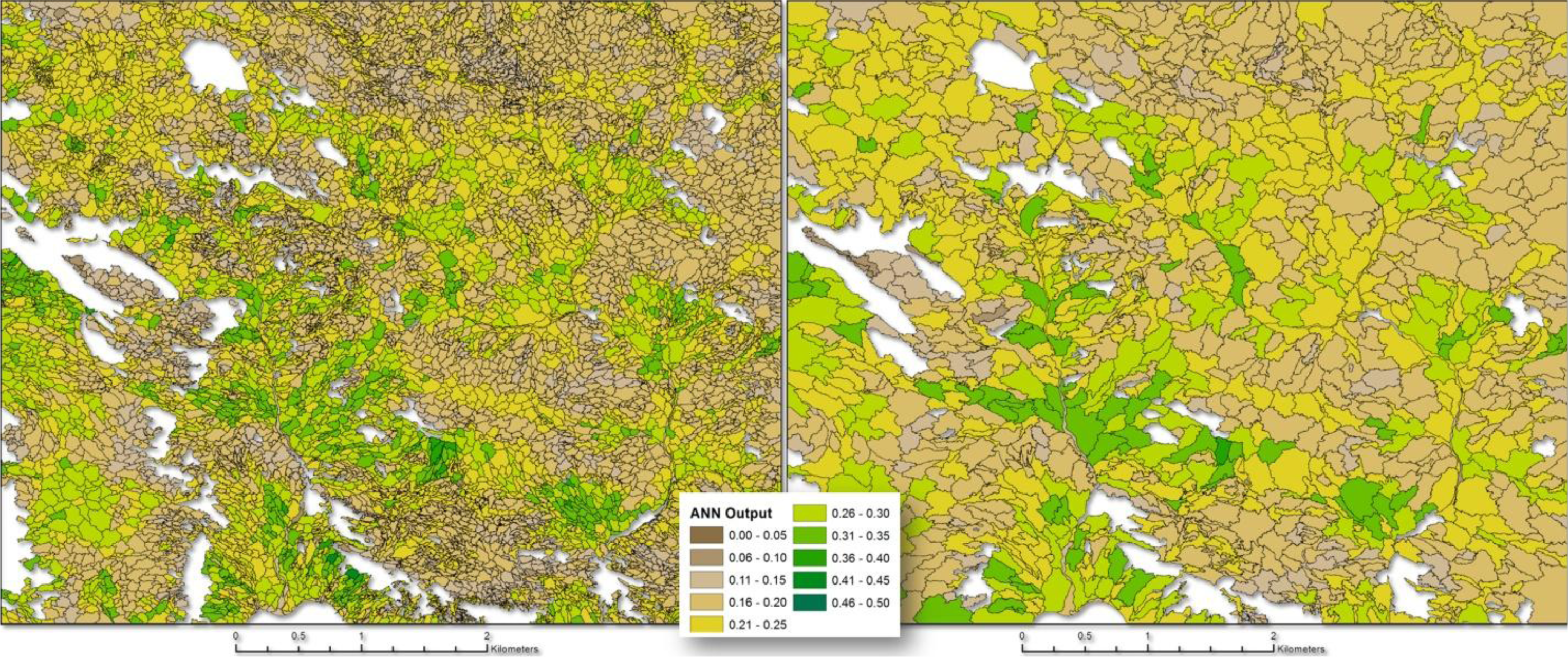
| SAR-Derived | DEM-Derived |
|---|---|
| Mean: U2 (13 August 2009) | TPI (150 m radius) |
| Mean: FQ5 (29 June 2009) | |
| Ln(NBRI): U75 (11 July 2010) U26 (9 July 2010) |
| Training | Validation | Testing | Final Output | |||||||
|---|---|---|---|---|---|---|---|---|---|---|
| Eco-Class | r2 | RMSE | r2 | RMSE | r2 | RMSE | r2 | N_RMSE | Mean SAVI | Mean ANN |
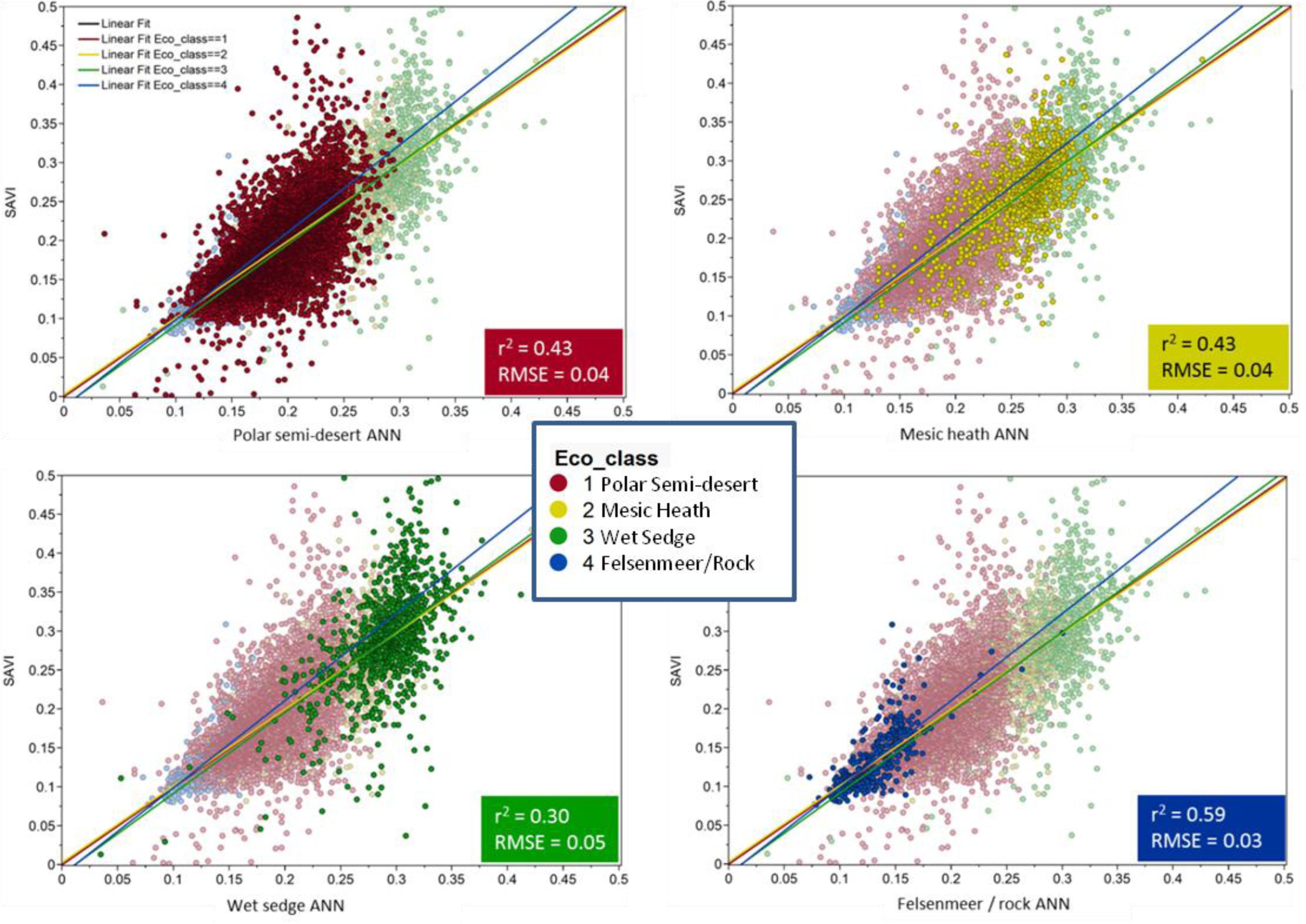
| Polar semi-desert | 0.43 | 0.039 | 0.44 | 0.038 | 0.44 | 0.038 | 0.43 | 8% | 0.189 | 0.190 |
| Mesic heath | 0.42 | 0.042 | 0.47 | 0.036 | 0.42 | 0.039 | 0.43 | 12% | 0.255 | 0.256 |
| Wet sedge | 0.28 | 0.053 | 0.30 | 0.048 | 0.37 | 0.058 | 0.30 | 11% | 0.291 | 0.292 |
| Felsenmeer/Rock | 0.61 | 0.025 | 0.50 | 0.030 | 0.57 | 0.021 | 0.59 | 11% | 0.137 | 0.133 |
| Combined Output | --- | --- | --- | --- | --- | --- | 0.60 | 8% | 0.204 | 0.205 |
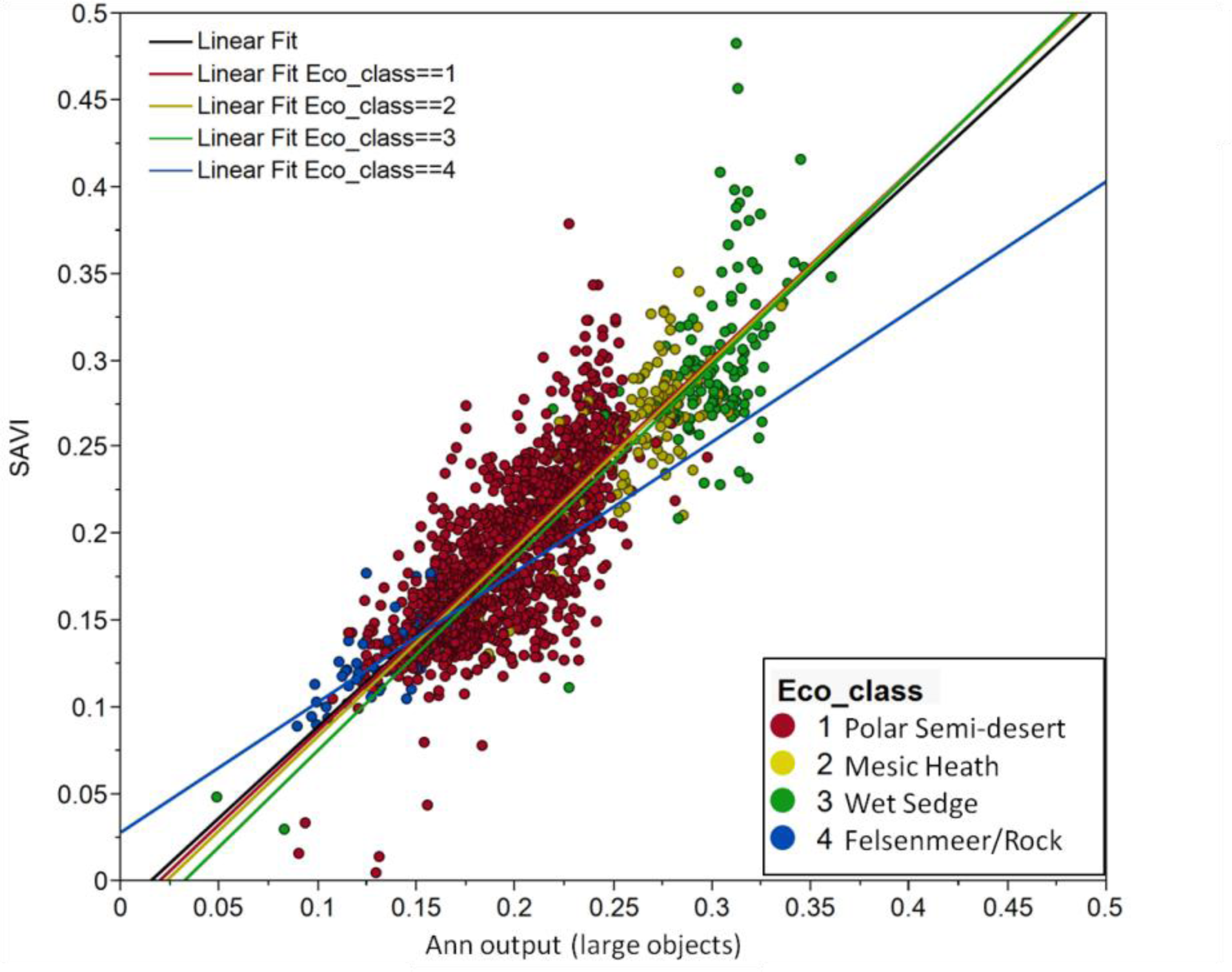
| All-class ANN | 0.49 | 0.046 | 0.48 | 0.046 | 0.49 | 0.046 | 0.49 | 9% | 0.204 | 0.205 |
| Eco-Class | r2 | N_RMSE | Mean SAVI | Mean ANN |
|---|---|---|---|---|
| Polar semi-desert | 0.56 | 8% | 0.190 | 0.196 |
| Mesic heath | 0.48 | 12% | 0.264 | 0.267 |
| Wet sedge | 0.52 | 9% | 0.294 | 0.297 |
| Felsenmeer/Rock | 0.47 | 19% | 0.128 | 0.133 |
| Combined | 0.72 | 6% | 0.203 | 0.208 |
© 2014 by the authors; licensee MDPI, Basel, Switzerland This article is an open access article distributed under the terms and conditions of the Creative Commons Attribution license (http://creativecommons.org/licenses/by/3.0/).
Share and Cite
Collingwood, A.; Treitz, P.; Charbonneau, F.; Atkinson, D.M. Artificial Neural Network Modeling of High Arctic Phytomass Using Synthetic Aperture Radar and Multispectral Data. Remote Sens. 2014, 6, 2134-2153. https://doi.org/10.3390/rs6032134
Collingwood A, Treitz P, Charbonneau F, Atkinson DM. Artificial Neural Network Modeling of High Arctic Phytomass Using Synthetic Aperture Radar and Multispectral Data. Remote Sensing. 2014; 6(3):2134-2153. https://doi.org/10.3390/rs6032134
Chicago/Turabian StyleCollingwood, Adam, Paul Treitz, Francois Charbonneau, and David M. Atkinson. 2014. "Artificial Neural Network Modeling of High Arctic Phytomass Using Synthetic Aperture Radar and Multispectral Data" Remote Sensing 6, no. 3: 2134-2153. https://doi.org/10.3390/rs6032134