Mapping Crop Cycles in China Using MODIS-EVI Time Series

 , and
, and
Abstract
:1. Introduction
2. Study Area and Materials
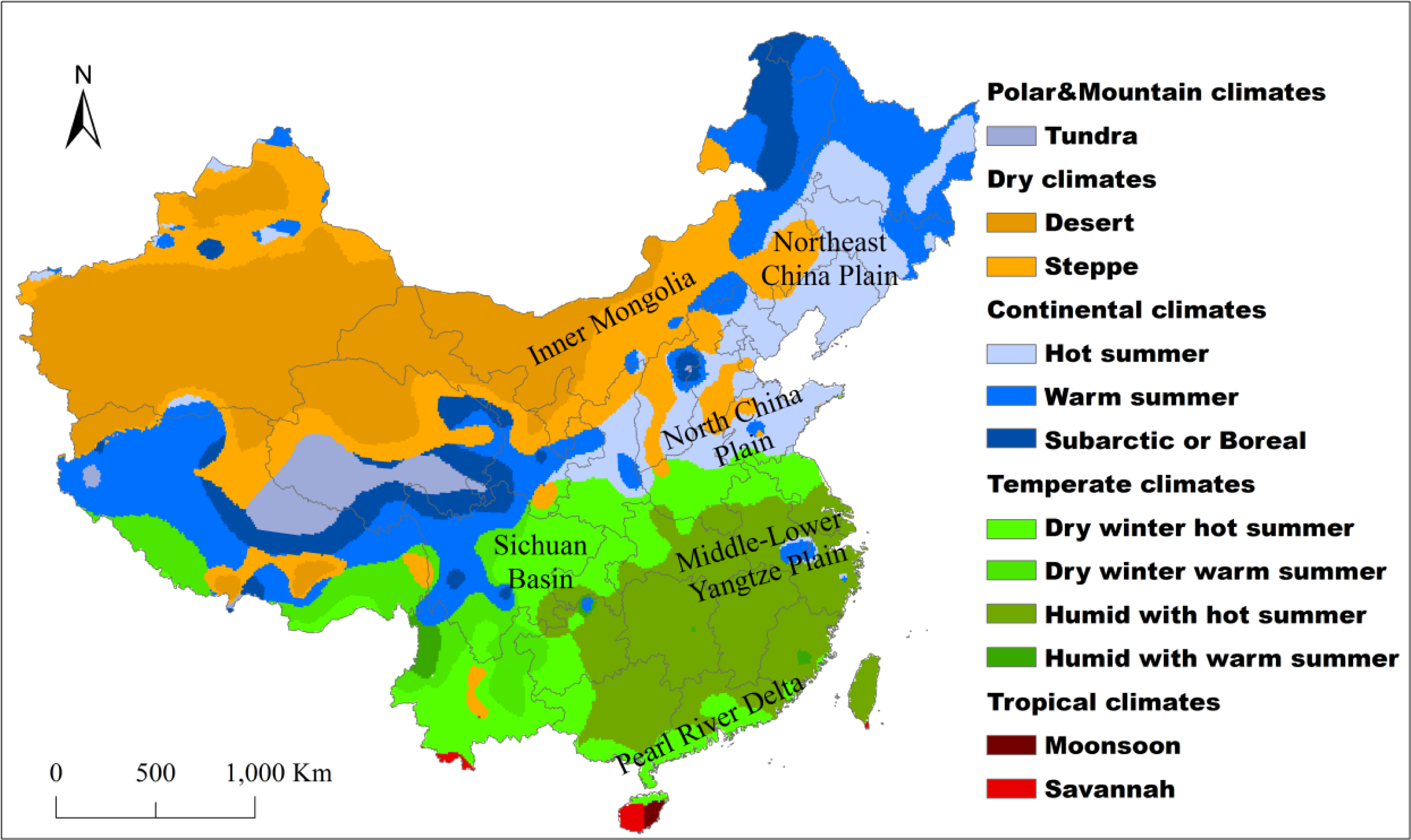
2.1. Description of the Study Area
2.2. MODIS Data
3. Methods
3.1. Preprocessing of MODIS Surface Reflectance Data
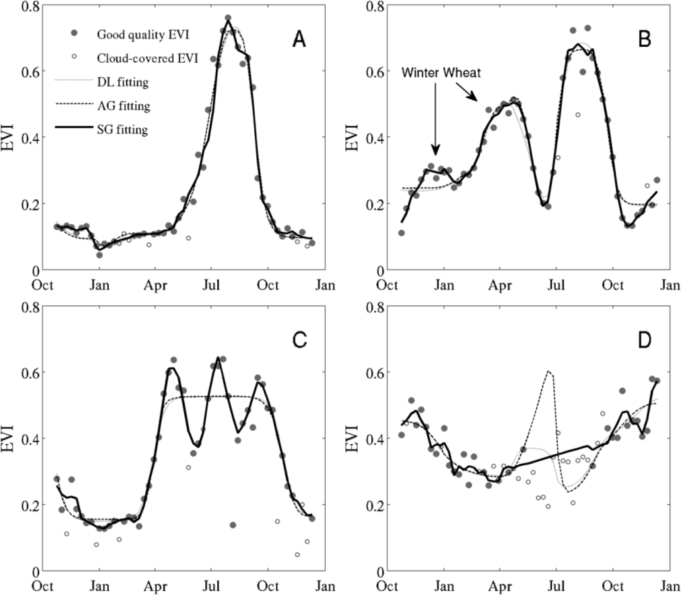
3.2. Time-Series Smoothing of MODIS EVI Data
3.3. Identifying Phenological Cycles Based on Smoothed MODIS EVI Time Series
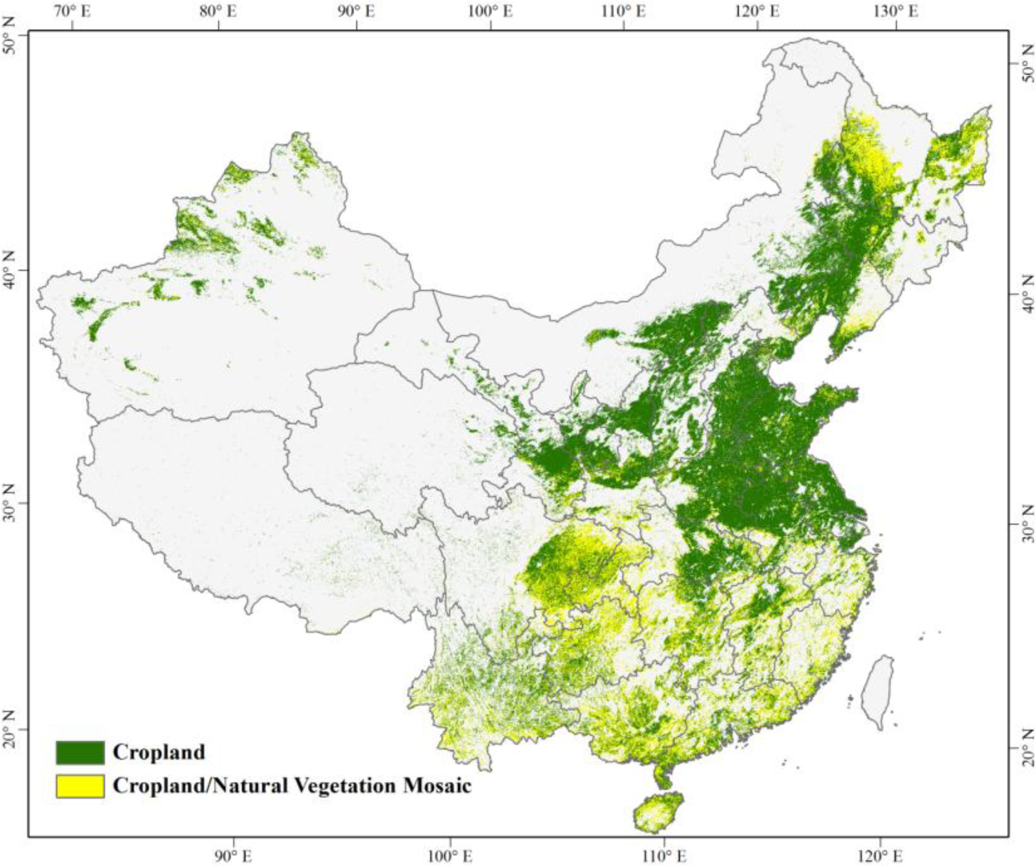
3.4. Mapping Agricultural Intensity by Incorporating Ancillary MODIS Data
3.5. Accuracy Assessment
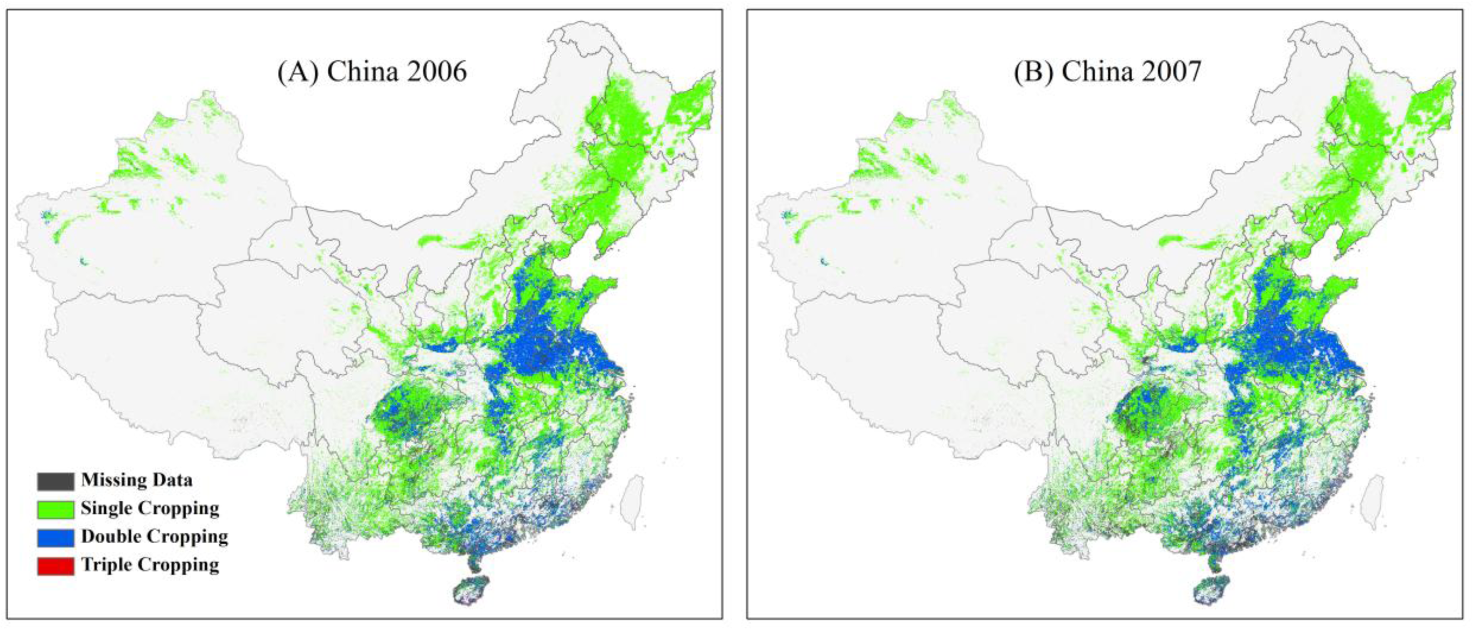
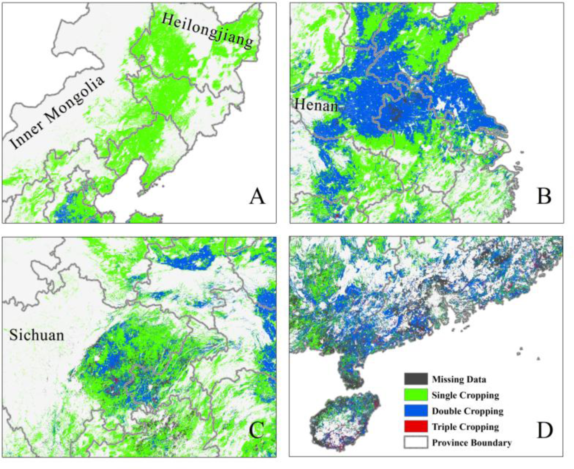
4. Results
5. Discussion
5.1. Factors That Influence the Mapping Accuracy
5.2. Potential Refinements
6. Conclusions
Acknowledgments
Author Contributions
Conflicts of Interest
References
- Pan, Y.; Li, L.; Zhang, J.; Liang, S.; Zhu, X.; Sulla-Menashe, D. Winter wheat area estimation from MODIS-EVI time series data using the Crop Proportion Phenology Index. Remote Sens. Environ 2012, 119, 232–242. [Google Scholar]
- Piao, S.; Ciais, P.; Huang, Y.; Shen, Z.; Peng, S.; Li, J.; Zhou, L.; Liu, H.; Ma, Y.; Ding, Y. The impacts of climate change on water resources and agriculture in China. Nature 2010, 467, 43–51. [Google Scholar]
- Zhang, X.; Friedl, M.A.; Schaaf, C.B.; Strahler, A.H.; Hodges, J.C.; Gao, F.; Reed, B.C.; Huete, A. Monitoring vegetation phenology using MODIS. Remote Sens. Environ 2003, 84, 471–475. [Google Scholar]
- Atzberger, C. Advances in remote sensing of agriculture: Context description, existing operational monitoring systems and major information needs. Remote Sens 2013, 5, 949–981. [Google Scholar]
- Justice, C.; Townshend, J.; Vermote, E.; Masuoka, E.; Wolfe, R.; Saleous, N.; Roy, D.; Morisette, J. An overview of MODIS land data processing and product status. Remote Sens. Environ 2002, 83, 3–15. [Google Scholar]
- Muchoney, D.; Borak, J.; Chi, H.; Friedl, M.; Gopal, S.; Hodges, J.; Morrow, N.; Strahler, A. Application of the MODIS global supervised classification model to vegetation and land cover mapping of central America. Int. J. Remote Sens 2000, 21, 1115–1138. [Google Scholar]
- Myneni, R.; Hoffman, S.; Knyazikhin, Y.; Privette, J.; Glassy, J.; Tian, Y.; Wang, Y.; Song, X.; Zhang, Y.; Smith, G. Global products of vegetation leaf area and fraction absorbed par from year one of MODIS data. Remote Sens. Environ 2002, 83, 214–231. [Google Scholar]
- Pittman, K.; Hansen, M.C.; Becker-Reshef, I.; Potapov, P.V.; Justice, C.O. Estimating global cropland extent with multi-year MODIS data. Remote Sens 2010, 2, 1844–1863. [Google Scholar]
- Friedl, M.A.; McIver, D.K.; Hodges, J.C.; Zhang, X.; Muchoney, D.; Strahler, A.H.; Woodcock, C.E.; Gopal, S.; Schneider, A.; Cooper, A. Global land cover mapping from MODIS: Algorithms and early results. Remote Sens. Environ 2002, 83, 287–302. [Google Scholar]
- Friedl, M.A.; Sulla-Menashe, D.; Tan, B.; Schneider, A.; Ramankutty, N.; Sibley, A.; Huang, X. MODIS collection 5 global land cover: Algorithm refinements and characterization of new datasets. Remote Sens. Environ 2010, 114, 168–182. [Google Scholar]
- Lim, Y.K.; Cai, M.; Kalnay, E.; Zhou, L. Observational evidence of sensitivity of surface climate changes to land types and urbanization. Geophys. Res. Lett 2005, 32. [Google Scholar] [CrossRef]
- Running, S.W.; Nemani, R.R.; Heinsch, F.A.; Zhao, M.; Reeves, M.; Hashimoto, H. A continuous satellite-derived measure of global terrestrial primary production. Bioscience 2004, 54, 547–560. [Google Scholar]
- Turner, D.P.; Ritts, W.D.; Cohen, W.B.; Gower, S.T.; Zhao, M.; Running, S.W.; Wofsy, S.C.; Urbanski, S.; Dunn, A.L.; Munger, J. Scaling gross primary production (GPP) over boreal and deciduous forest landscapes in support of MODIS GPP product validation. Remote Sens. Environ 2003, 88, 256–270. [Google Scholar]
- Monfreda, C.; Ramankutty, N.; Foley, J.A. Farming the planet: 2. Geographic distribution of crop areas, yields, physiological types, and net primary production in the year 2000. Global Biogeochem. Cycle 2008, 22. [Google Scholar] [CrossRef]
- Ramankutty, N.; Evan, A.T.; Monfreda, C.; Foley, J.A. Farming the planet: 1. Geographic distribution of global agricultural lands in the year 2000. Global Biogeochem. Cycles 2008, 22. [Google Scholar] [CrossRef]
- Pervez, M.S.; Brown, J.F. Mapping irrigated lands at 250-m scale by merging MODIS data and national agricultural statistics. Remote Sens 2010, 2, 2388–2412. [Google Scholar]
- You, X.; Meng, J.; Zhang, M.; Dong, T. Remote sensing based detection of crop phenology for agricultural zones in China using a new threshold method. Remote Sens 2013, 5, 3190–3211. [Google Scholar]
- Doll, P.; Siebert, S. Global modeling of irrigation water requirements. Water Resour. Res 2002, 38. [Google Scholar] [CrossRef]
- Foley, J.A.; DeFries, R.; Asner, G.P.; Barford, C.; Bonan, G.; Carpenter, S.R.; Chapin, F.S.; Coe, M.T.; Daily, G.C.; Gibbs, H.K. Global consequences of land use. Science 2005, 309, 570–574. [Google Scholar]
- Tilman, D.; Fargione, J.; Wolff, B.; D’Antonio, C.; Dobson, A.; Howarth, R.; Schindler, D.; Schlesinger, W.H.; Simberloff, D.; Swackhamer, D. Forecasting agriculturally driven global environmental change. Science 2001, 292, 281–284. [Google Scholar]
- Xin, Q.; Gong, P.; Yu, C.; Yu, L.; Broich, M.; Suyker, A.E.; Myneni, R.B. A production efficiency model-based method for satellite estimates of corn and soybean yields in the midwestern US. Remote Sens 2013, 5, 5926–5943. [Google Scholar]
- Frolking, S.; Qiu, J.; Boles, S.; Xiao, X.; Liu, J.; Zhuang, Y.; Li, C.; Qin, X. Combining remote sensing and ground census data to develop new maps of the distribution of rice agriculture in China. Global Biogeochem. Cycle 2002, 16. [Google Scholar] [CrossRef]
- Siebert, S.; Portmann, F.T.; Doll, P. Global patterns of cropland use intensity. Remote Sens 2010, 2, 1625–1643. [Google Scholar]
- Xiao, X.; Boles, S.; Frolking, S.; Li, C.; Babu, J.Y.; Salas, W.; Moore, B., III. Mapping paddy rice agriculture in south and southeast Asia using multi-temporal MODIS images. Remote Sens. Environ 2006, 100, 95–113. [Google Scholar]
- Yu, L.; Wang, J.; Clinton, N.; Xin, Q.; Zhong, L.; Chen, Y.; Gong, P. FROM-GC: 30 m global cropland extent derived through multi-source data integration. Int. J. Digit. Earth 2013, 6. doi: 0.1080/17538947.2013.822574. [Google Scholar]
- Hertel, T.W.; Burke, M.B.; Lobell, D.B. The poverty implications of climate-induced crop yield changes by 2030. Global Environ. Change 2010, 20, 577–585. [Google Scholar]
- Ganguly, S.; Friedl, M.A.; Tan, B.; Zhang, X.; Verma, M. Land surface phenology from MODIS: Characterization of the collection 5 global land cover dynamics product. Remote Sens. Environ 2010, 114, 1805–1816. [Google Scholar]
- Liu, J.; Zhu, W.; Cui, X. A shape-matching cropping index (CI) mapping method to determine agricultural cropland intensities in China using MODIS time-series data. Photogramm. Eng. Remote Sens 2012, 78, 829–837. [Google Scholar]
- Tan, B.; Morisette, J.T.; Wolfe, R.E.; Gao, F.; Ederer, G.A.; Nightingale, J.; Pedelty, J.A. An enhanced timesat algorithm for estimating vegetation phenology metrics from MODIS data. IEEE J. STARS 2011, 4, 361–371. [Google Scholar]
- Galford, G.L.; Mustard, J.F.; Melillo, J.; Gendrin, A.; Cerri, C.C.; Cerri, C.E. Wavelet analysis of MODIS time series to detect expansion and intensification of row-crop agriculture in Brazil. Remote Sens. Environ 2008, 112, 576–587. [Google Scholar]
- Potgieter, A.; Apan, A.; Hammer, G.; Dunn, P. Early-season crop area estimates for winter crops in NE Australia using MODIS satellite imagery. ISPRS J. Photogramm. Remote Sens 2010, 65, 380–387. [Google Scholar]
- Wardlow, B.D.; Egbert, S.L. Large-area crop mapping using time-series MODIS 250 m NDVI data: An assessment for the US central great plains. Remote Sens. Environ 2008, 112, 1096–1116. [Google Scholar]
- Huete, A.; Didan, K.; Miura, T.; Rodriguez, E.P.; Gao, X.; Ferreira, L.G. Overview of the radiometric and biophysical performance of the MODIS vegetation indices. Remote Sens. Environ 2002, 83, 195–213. [Google Scholar]
- Sakamoto, T.; van Phung, C.; Kotera, A.; Nguyen, K.D.; Yokozawa, M. Analysis of rapid expansion of inland aquaculture and triple rice-cropping areas in a coastal area of the Vietnamese Mekong Delta using MODIS time-series imagery. Landscape Urban Plan 2009, 92, 34–46. [Google Scholar]
- Li, X.; Wang, X. Changes in agricultural land use in China: 1981–2000. Asian Geogr 2003, 22, 27–42. [Google Scholar]
- Lobell, D.B.; Asner, G.P. Cropland distributions from temporal unmixing of MODIS data. Remote Sens. Environ 2004, 93, 412–422. [Google Scholar]
- Ozdogan, M. The spatial distribution of crop types from MODIS data: Temporal unmixing using independent component analysis. Remote Sens. Environ 2010, 114, 1190–1204. [Google Scholar]
- Ozdogan, M.; Woodcock, C.E. Resolution dependent errors in remote sensing of cultivated areas. Remote Sens. Environ 2006, 103, 203–217. [Google Scholar]
- Roy, D.; Lewis, P.; Schaaf, C.; Devadiga, S.; Boschetti, L. The global impact of clouds on the production of MODIS bidirectional reflectance model-based composites for terrestrial monitoring. IEEE Geosci. Remote Sens. Lett 2006, 3, 452–456. [Google Scholar]
- Tan, B.; Woodcock, C.; Hu, J.; Zhang, P.; Ozdogan, M.; Huang, D.; Yang, W.; Knyazikhin, Y.; Myneni, R. The impact of gridding artifacts on the local spatial properties of MODIS data: Implications for validation, compositing, and band-to-band registration across resolutions. Remote Sens. Environ 2006, 105, 98–114. [Google Scholar]
- Ren, J.; Chen, Z.; Zhou, Q.; Tang, H. Regional yield estimation for winter wheat with MODIS-NDVI data in Shandong, China. Int. J. Appl. Earth Obs. Geoinf 2008, 10, 403–413. [Google Scholar]
- Peel, M.C.; Finlayson, B.L.; McMahon, T.A. Updated world map of the Koppen-Geiger climate classification. Hydrol. Earth Syst. Sci. Discuss 2007, 4, 439–473. [Google Scholar]
- The USGS EROS Data Center. Available online: http://eros.usgs.gov/ (accessed on 30 December 2013).
- Vermote, E.F.; El Saleous, N.Z.; Justice, C.O. Atmospheric correction of MODIS data in the visible to middle infrared: First results. Remote Sens. Environ 2002, 83, 97–111. [Google Scholar]
- Wan, Z.; Zhang, Y.; Zhang, Q.; Li, Z.L. Validation of the land-surface temperature products retrieved from Terra Moderate Resolution Imaging Spectroradiometer data. Remote Sens. Environ 2002, 83, 163–180. [Google Scholar]
- Loveland, T.; Belward, A. The IGBP-DIS global 1km land cover data set, DISCover: First results. Int. J. Remote Sens 1997, 18, 3289–3295. [Google Scholar]
- The USGS Website. Available online: https://lpdaac.usgs.gov/ (accessed on 30 December 2013).
- Roy, D.P.; Borak, J.S.; Devadiga, S.; Wolfe, R.E.; Zheng, M.; Descloitres, J. The MODIS land product quality assessment approach. Remote Sens. Environ 2002, 83, 62–76. [Google Scholar]
- Grogan, K.; Fensholt, R. Exploring patterns and effects of aerosol quantity flag anomalies in MODIS surface reflectance products in the tropics. Remote Sens 2013, 5, 3495–3515. [Google Scholar]
- Chen, J.; Jonsson, P.; Tamura, M.; Gu, Z.; Matsushita, B.; Eklundh, L. A simple method for reconstructing a high-quality NDVI time-series data set based on the Savitzky-Golay filter. Remote Sens. Environ 2004, 91, 332–344. [Google Scholar]
- Sakamoto, T.; Yokozawa, M.; Toritani, H.; Shibayama, M.; Ishitsuka, N.; Ohno, H. A crop phenology detection method using time-series MODIS data. Remote Sens. Environ 2005, 96, 366–374. [Google Scholar]
- Jonsson, P.; Eklundh, L. Timesat—A program for analyzing time-series of satellite sensor data. Comput. Geosci 2004, 30, 833–845. [Google Scholar]
- Jonsson, P.; Eklundh, L. Seasonality extraction by function fitting to time-series of satellite sensor data. IEEE Trans. Geosci. Remote Sens 2002, 40, 1824–1832. [Google Scholar]
- Becker-Reshef, I.; Vermote, E.; Lindeman, M.; Justice, C. A generalized regression-based model for forecasting winter wheat yields in Kansas and Ukraine using MODIS data. Remote Sens. Environ 2010, 114, 1312–1323. [Google Scholar]
- Jolly, W.M.; Nemani, R.; Running, S.W. A generalized, bioclimatic index to predict foliar phenology in response to climate. Glob. Chang. Biol 2005, 11, 619–632. [Google Scholar]
- Larcher, W.; Bauer, H. Ecological Significance of Resistance to Low Temperature. In Physiological Plant Ecology I; Lange, O.L., Nobel, P.S., Osmond, C.B., Ziegler, H., Eds.; Springer: Heidelberg, Germany, 1981; pp. 403–437. [Google Scholar]
- Li, A.; Liang, S.; Wang, A.; Qin, J. Estimating crop yield from multi-temporal satellite data using multivariate regression and neural network techniques. Photogramm. Eng. Remote Sens 2007, 73, 1149–1157. [Google Scholar]
- Sari, D.K.; Ismullah, I.H.; Sulasdi, W.N.; Harto, A.B. Detecting rice phenology in paddy fields with complex cropping pattern using time series MODIS data. ITB J. Sci 2010, 42, 91–106. [Google Scholar]
- Lobell, D.B.; Schlenker, W.; Costa-Roberts, J. Climate trends and global crop production since 1980. Science 2011, 333, 616–620. [Google Scholar]
- National Bureau of Statistics of China. Available online: http://www.stats.gov.cn/tjsj/ndsj/ (accessed on 30 December 2013).
- Seto, K.C.; Kaufmann, R.K.; Woodcock, C.E. Landsat reveals China’s farmland reserves, but they’re vanishing fast. Nature 2000, 406. [Google Scholar] [CrossRef]
- Smil, V. China’s agricultural land. China Q 1999, 158, 414–429. [Google Scholar]
- Congalton, R.G.; Green, K. A practical look at the sources of confusion in error matrix generation. Photogramm. Eng. Remote Sens 1993, 59, 641–644. [Google Scholar]
- Gong, P.; Wang, J.; Yu, L.; Zhao, Y.; Zhao, Y.; Liang, L.; Niu, Z.; Huang, X.; Fu, H.; Liu, S. Finer resolution observation and monitoring of global land cover: First mapping results with Landsat TM and ETM+ data. Int. J. Remote Sens 2013, 34, 2607–2654. [Google Scholar]
- World Agriculture: Towards 2010. Available online: https://www.mpl.ird.fr/crea/taller-colombia/FAO/AGLL/pdfdocs/wat2010.pdf (accessed on 30 December 2013).
- Ellis, E.C. Long-Term Ecological Changes in the Densely Populated Rural Landscapes of China. In Ecosystems and Land Use Change; Defries, S.R., Asner, G.P., Houghton, R.A., Eds.; American Geophysical Union: Washington, DC, USA, 2013. [Google Scholar]
- Podwysocki, M.H. Analysis of Field Size Distributions, Lacie Test Sites 5029, 5033, and 5039, Anhwei Province, People’s Republic of China; Report No. N76-27652/6; U.S. Department of Commerce: Virgunua, VI, USA, 1976. [Google Scholar]
- Hilker, T.; Wulder, M.A.; Coops, N.C.; Linke, J.; McDermid, G.; Masek, J.G.; Gao, F.; White, J.C. A new data fusion model for high spatial-and temporal-resolution mapping of forest disturbance based on Landsat and MODIS. Remote Sens. Environ 2009, 113, 1613–1627. [Google Scholar]
- Xin, Q.; Olofsson, P.; Zhu, Z.; Tan, B.; Woodcock, C.E. Toward near real-time monitoring of forest disturbance by fusion of MODIS and Landsat data. Remote Sens. Environ. 2013, 135, 234–247. [Google Scholar]
- Ozdogan, M.; Yang, Y.; Allez, G.; Cervantes, C. Remote sensing of irrigated agriculture: Opportunities and challenges. Remote Sens 2010, 2, 2274–2304. [Google Scholar]
- Turner, D.P.; Gower, S.T.; Cohen, W.B.; Gregory, M.; Maiersperger, T.K. Effects of spatial variability in light use efficiency on satellite-based NPP monitoring. Remote Sens. Environ 2002, 80, 397–405. [Google Scholar]
- Woodcock, C.E.; Strahler, A.H. The factor of scale in remote sensing. Remote Sens. Environ 1987, 21, 311–332. [Google Scholar]
- Gislason, P.O.; Benediktsson, J.A.; Sveinsson, J.R. Random forests for land cover classification. Pattern Recognit. Lett 2006, 27, 294–300. [Google Scholar]
- Gopal, S.; Woodcock, C.E.; Strahler, A.H. Fuzzy neural network classification of global land cover from a 1 AVHRR data set. Remote Sens. Environ 1999, 67, 230–243. [Google Scholar]
Appendix Sample Points for Accuracy Assessment


| Province | Arable Land (kha) | Gross Sown Area (kha) | Cropping Indexb (100%) |
|---|---|---|---|
| Beijing | 343.9 | 318.0 | 92.5% |
| Tianjin | 485.6 | 499.4 | 102.8% |
| Hebei | 6883.3 | 8785.5 | 127.6% |
| Shanxi | 4588.6 | 3795.4 | 82.7% |
| Inner Mongolia | 8201.0 | 6215.7 | 75.8% |
| Liaoning | 4174.8 | 3796.7 | 90.9% |
| Jilin | 5578.4 | 4954.1 | 88.8% |
| Heilongjiang | 11,773.0 | 10,083.7 | 85.7% |
| Shanghai | 315.1 | 403.6 | 128.1% |
| Jiangsu | 5061.7 | 7641.2 | 151.0% |
| Zhejiang | 2125.3 | 2837.9 | 133.5% |
| Anhui | 5971.7 | 9172.5 | 153.6% |
| Fujian | 1434.7 | 2481.3 | 172.9% |
| Jiangxi | 2993.4 | 5251.4 | 175.4% |
| Shandong | 7689.3 | 10,736.1 | 139.6% |
| Henan | 8110.3 | 13,922.7 | 171.7% |
| Hubei | 4949.5 | 7279.4 | 147.1% |
| Hunan | 3953.0 | 7977.6 | 201.8% |
| Guangdong | 3272.2 | 4815.4 | 147.2% |
| Guangxi | 4407.9 | 6489.2 | 147.2% |
| Hainan | 762.1 | 778.1 | 102.1% |
| Chongqing | 2067.6 | 3487.7 | 168.7% |
| Sichuan | 9169.1 | 9480.2 | 103.4% |
| Guizhou | 4903.5 | 4804.1 | 98.0% |
| Yunnan | 6421.6 | 6053.8 | 94.3% |
| Tibet | 362.6 | 235.0 | 64.8% |
| Shaanxi | 5140.5 | 4201.8 | 81.7% |
| Gansu | 5024.7 | 3726.0 | 74.2% |
| Qinghai | 688.0 | 476.7 | 69.3% |
| Ningxia | 1268.8 | 1099.3 | 86.6% |
| Xinjiang | 3985.7 | 3731.2 | 93.6% |
| Year | R2 | RMSE (1000 kha) | ME (1000 kha) |
|---|---|---|---|
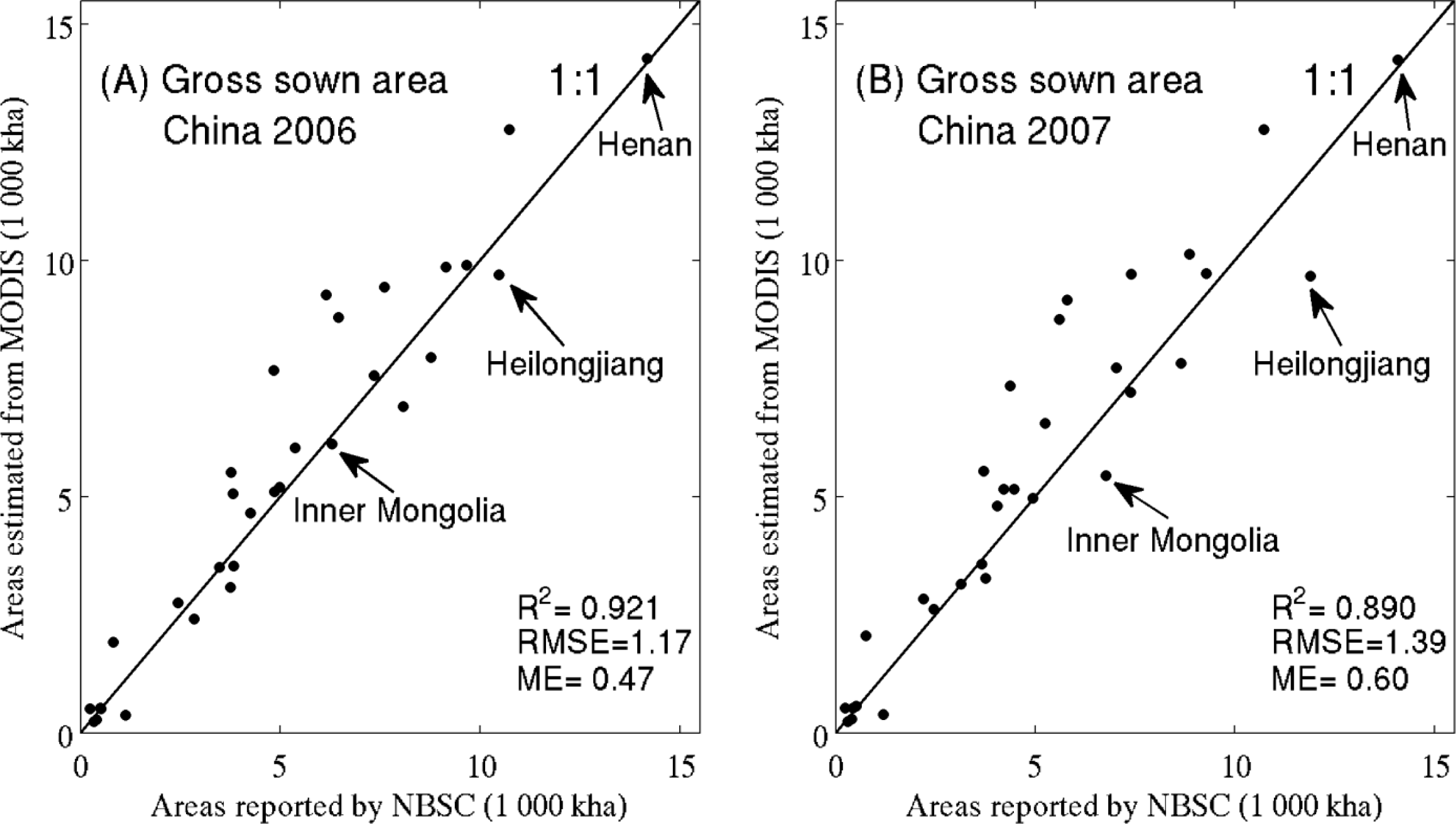
| 2006 | 0.921 | 1.17 | 0.47 |
| 2007 | 0.890 | 1.39 | 0.60 |
| 2008 | 0.899 | 1.38 | 0.59 |
| 2009 | 0.859 | 1.48 | 0.38 |
| 2010 | 0.897 | 1.24 | 0.29 |
| 2011 | 0.886 | 1.31 | 0.31 |
| Land Use Classes | Visual Interpretation of MODIS EVI Time Series | User’s Accuracy | |||
|---|---|---|---|---|---|
| Non-Cropping | Single-Cropping | Double-Cropping | Triple-Cropping | ||
| non-cropping | 0 | 0 | 0 | 0 | |
| single-cropping | 1 | 1392 | 100 | 7 | 92.8% |
| double-cropping | 0 | 101 | 1359 | 40 | 90.6% |
| triple-cropping | 0 | 35 | 120 | 1345 | 89.7% |
| Producer’s accuracy | 91.1% | 86.1% | 96.6% | ||
| overall accuracy = 91.0% | |||||
© 2014 by the authors; licensee MDPI, Basel, Switzerland This article is an open access article distributed under the terms and conditions of the Creative Commons Attribution license (http://creativecommons.org/licenses/by/3.0/).
Share and Cite
Li, L.; Friedl, M.A.; Xin, Q.; Gray, J.; Pan, Y.; Frolking, S. Mapping Crop Cycles in China Using MODIS-EVI Time Series. Remote Sens. 2014, 6, 2473-2493. https://doi.org/10.3390/rs6032473
Li L, Friedl MA, Xin Q, Gray J, Pan Y, Frolking S. Mapping Crop Cycles in China Using MODIS-EVI Time Series. Remote Sensing. 2014; 6(3):2473-2493. https://doi.org/10.3390/rs6032473
Chicago/Turabian StyleLi, Le, Mark A. Friedl, Qinchuan Xin, Josh Gray, Yaozhong Pan, and Steve Frolking. 2014. "Mapping Crop Cycles in China Using MODIS-EVI Time Series" Remote Sensing 6, no. 3: 2473-2493. https://doi.org/10.3390/rs6032473