Regional Water Balance Based on Remotely Sensed Evapotranspiration and Irrigation: An Assessment of the Haihe Plain, China


Abstract
:1. Introduction
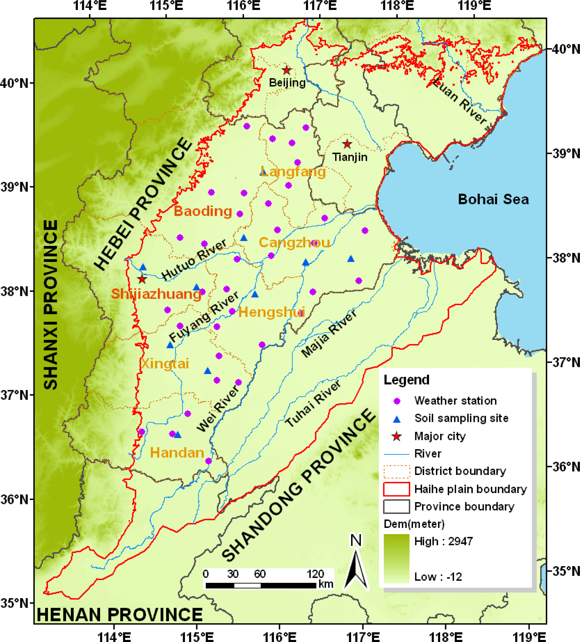
2. Study Area
3. Model Description
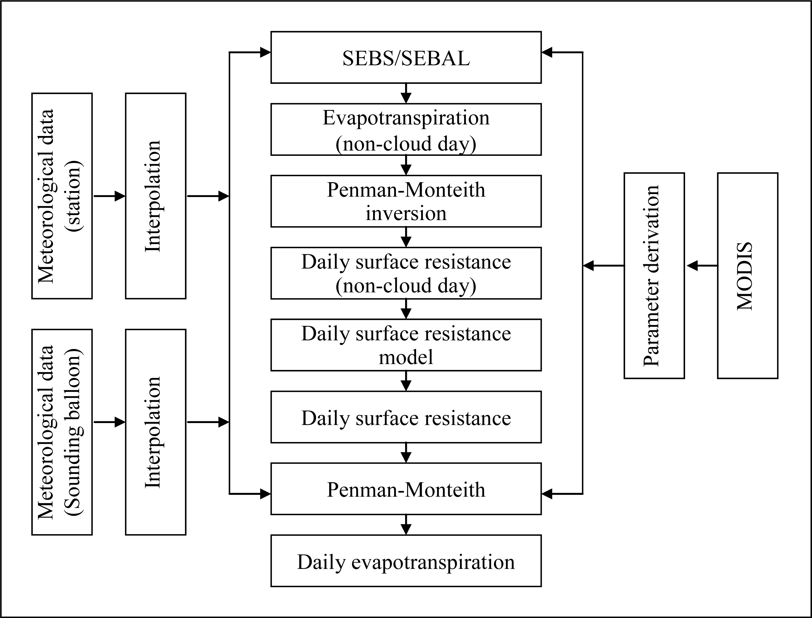
3.1. ETWatch
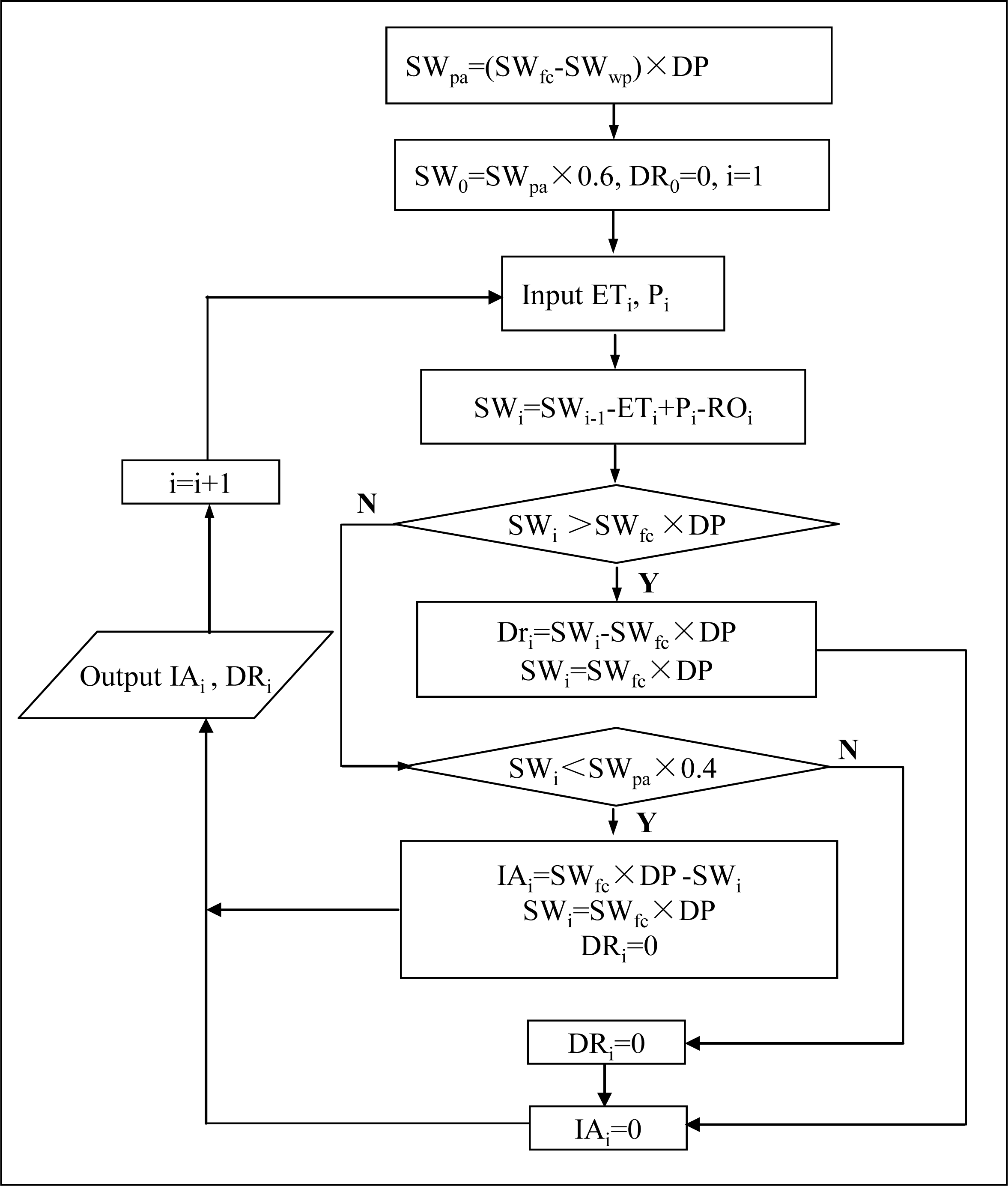
3.2. Irrigation Applied (IA) Estimation Model
4. Data Collection
4.1. Remote Sensing Data
4.2. Meteorological Data
4.3. Lysimeter Data
5. Results
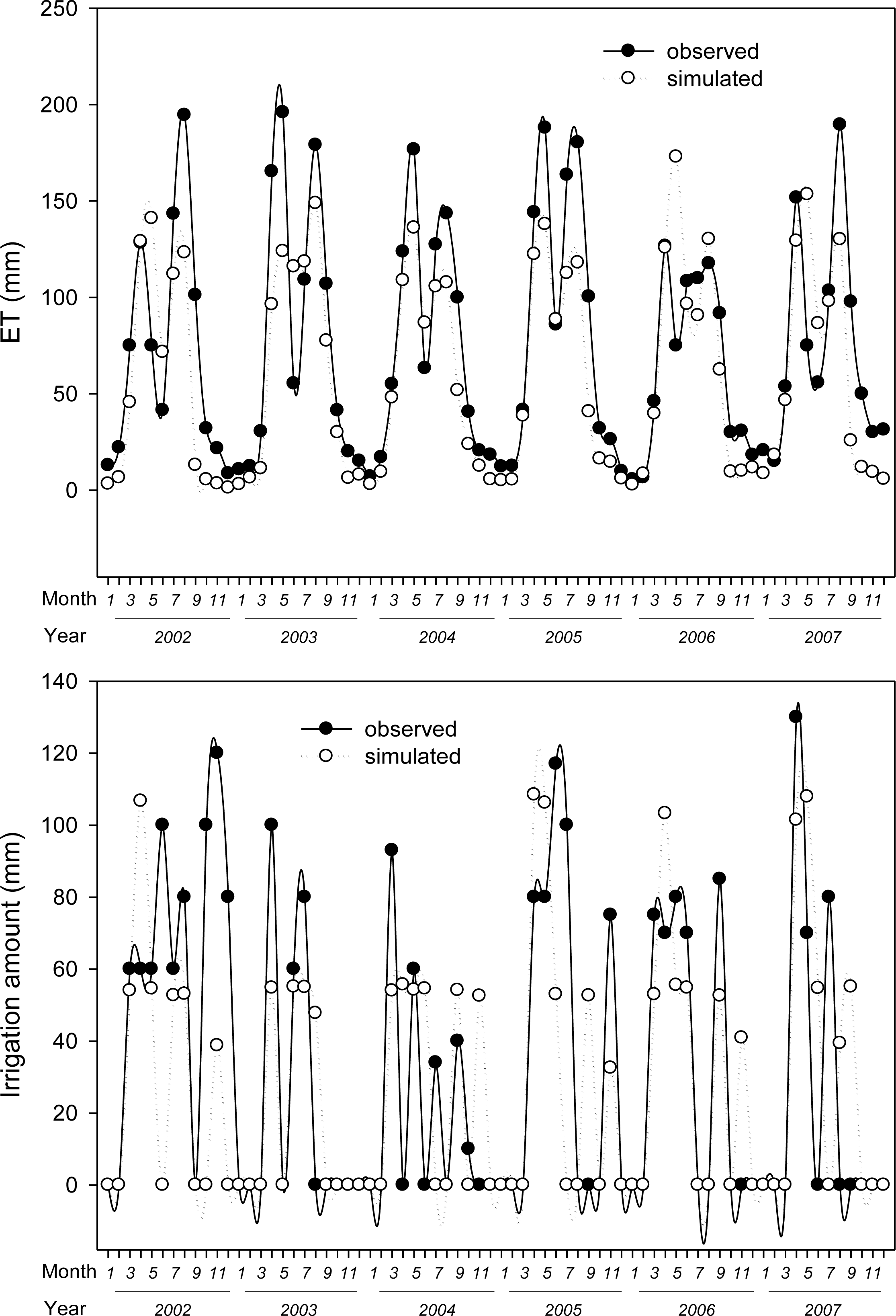
5.1. Verification
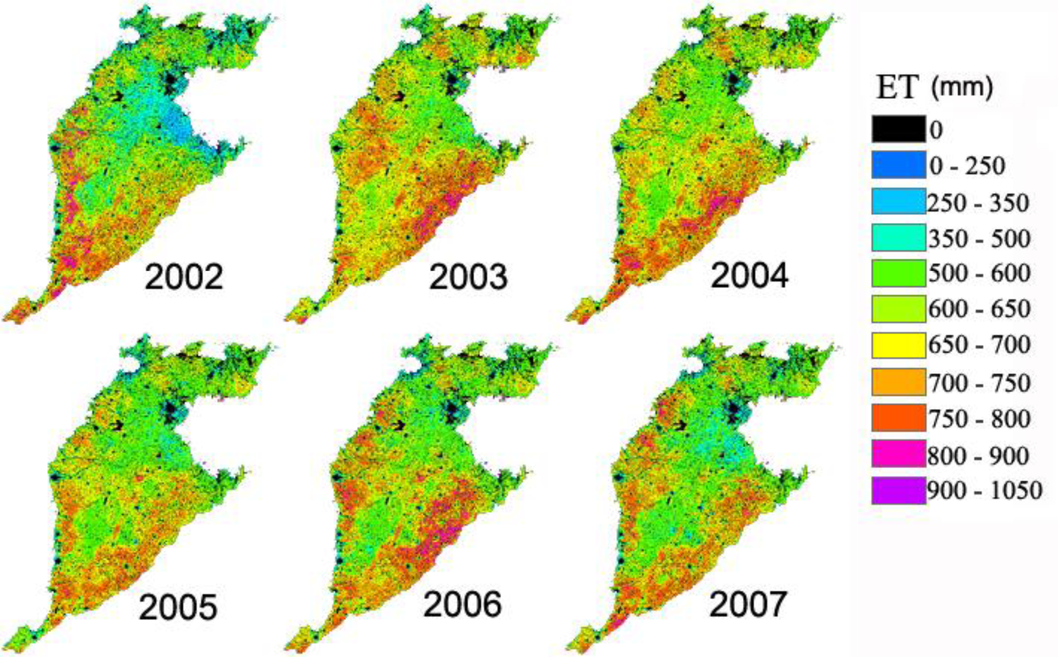
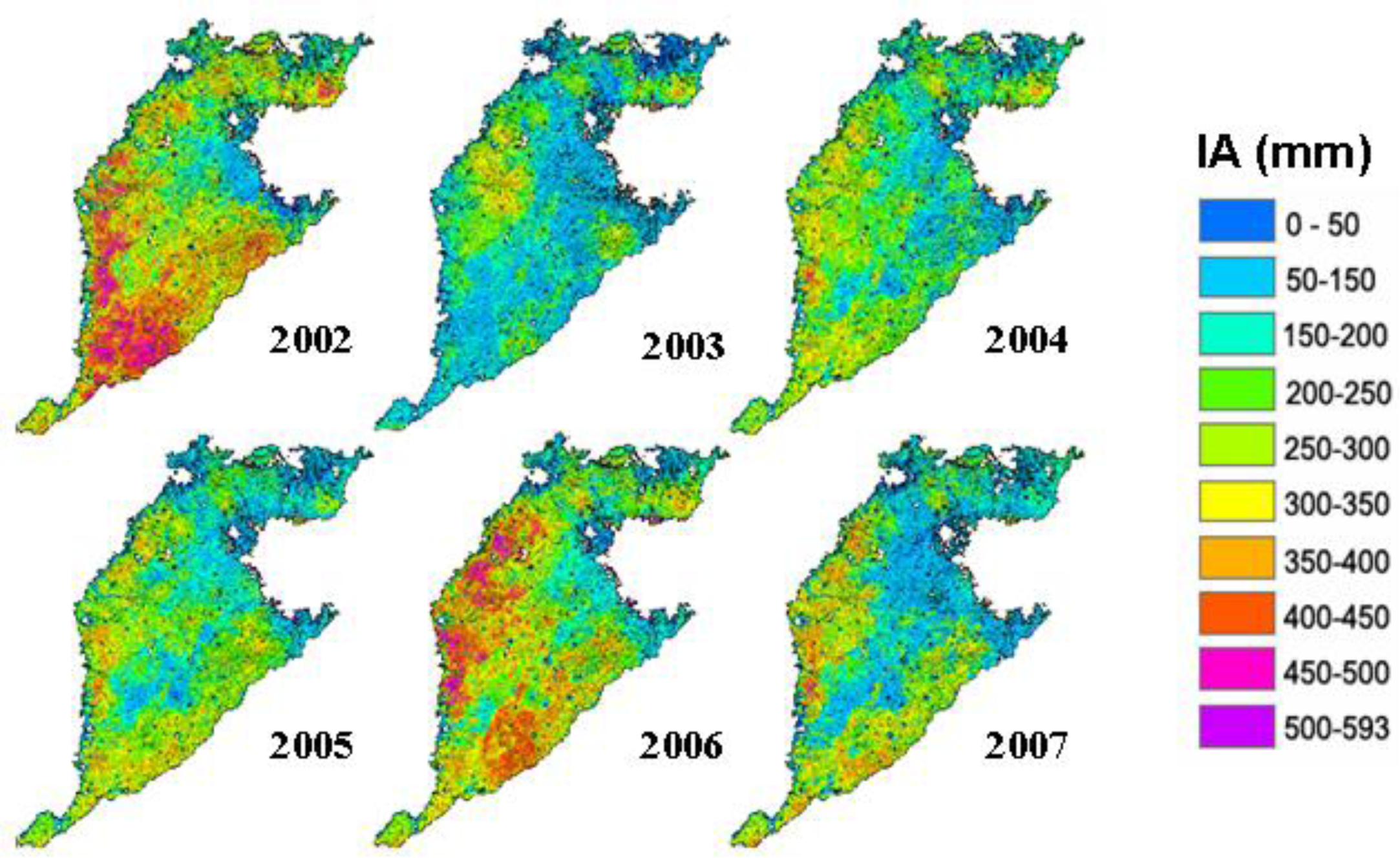
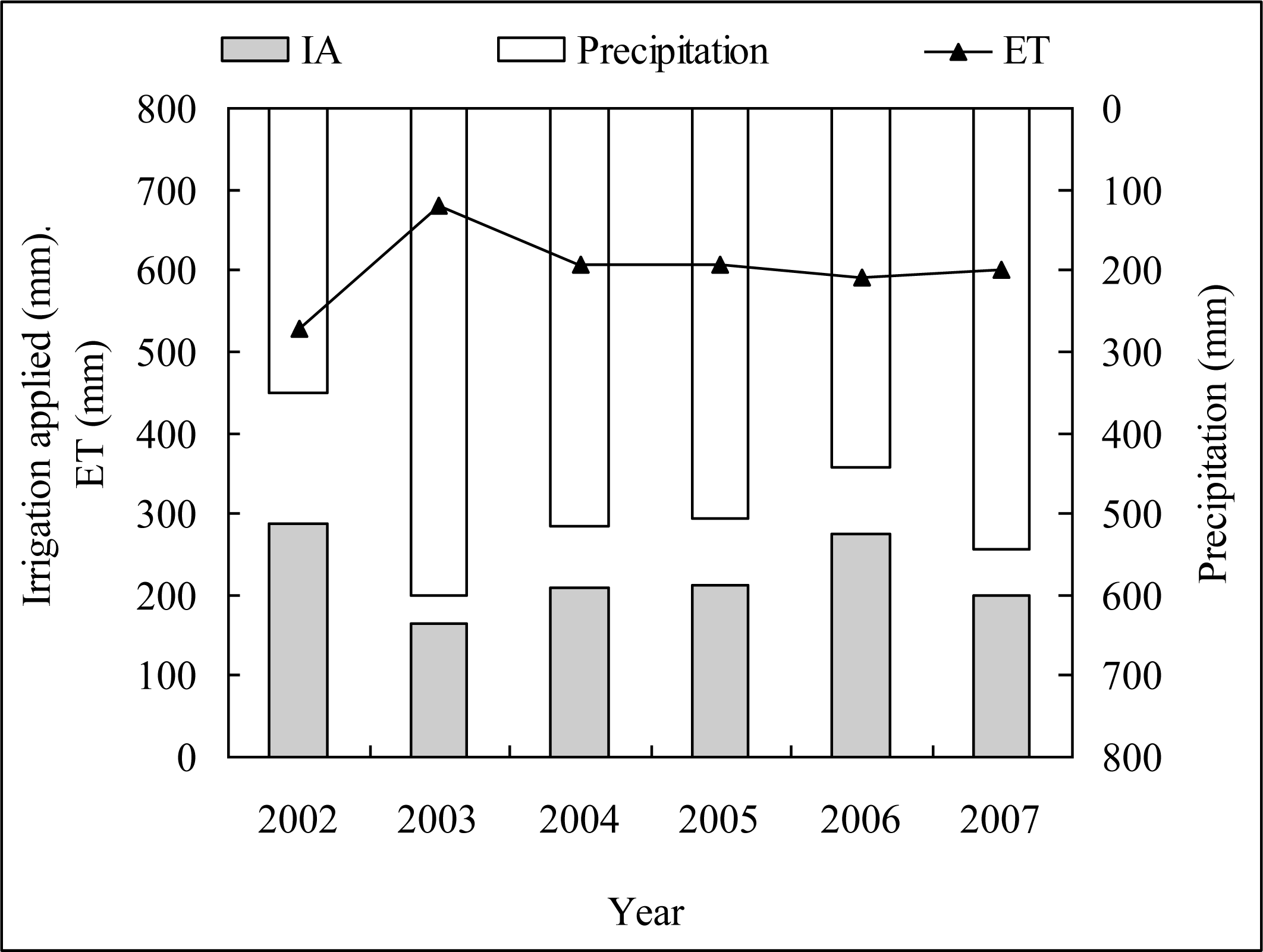
5.2. Yearly Spatial Distribution of ET and IA
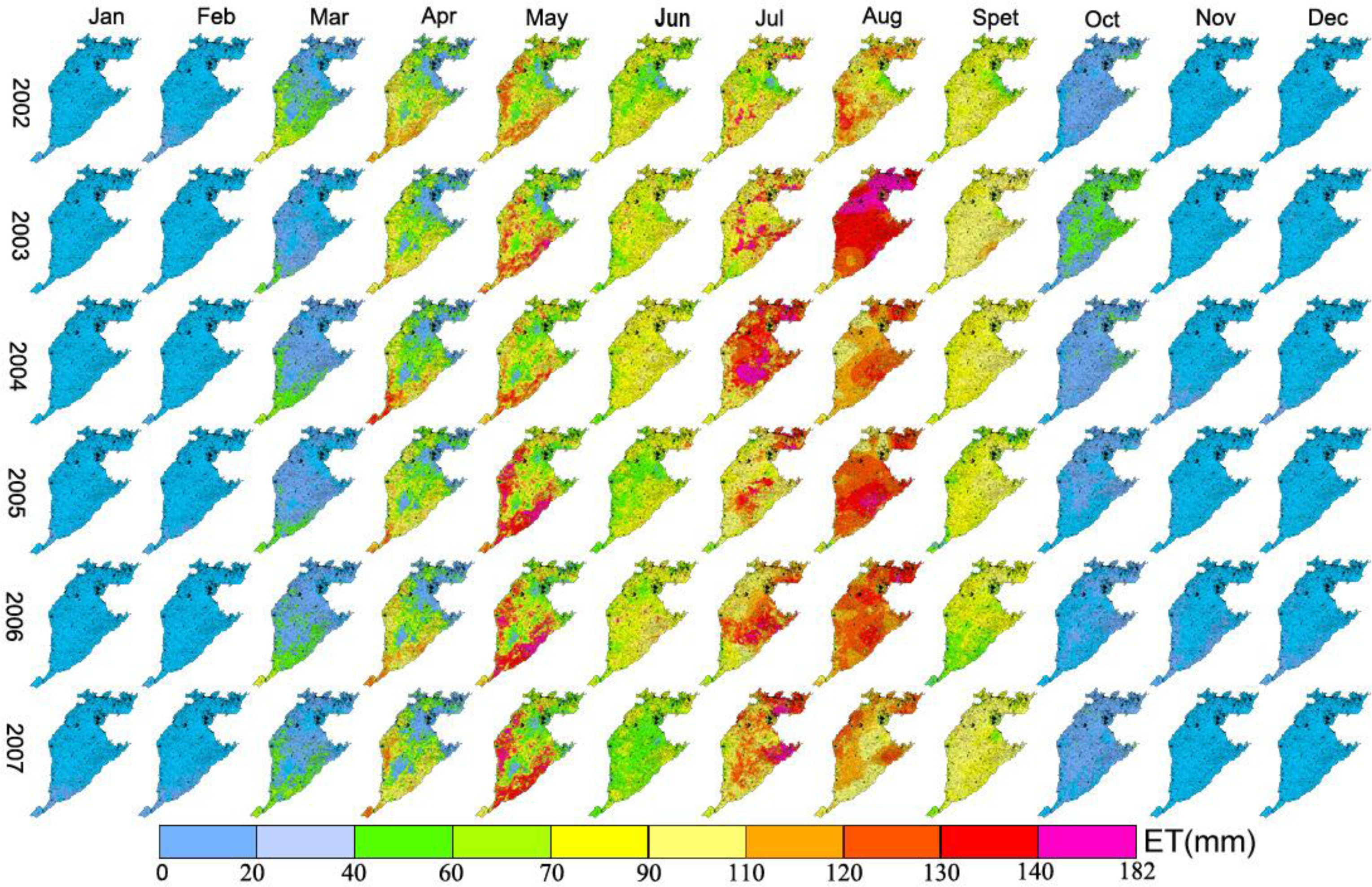
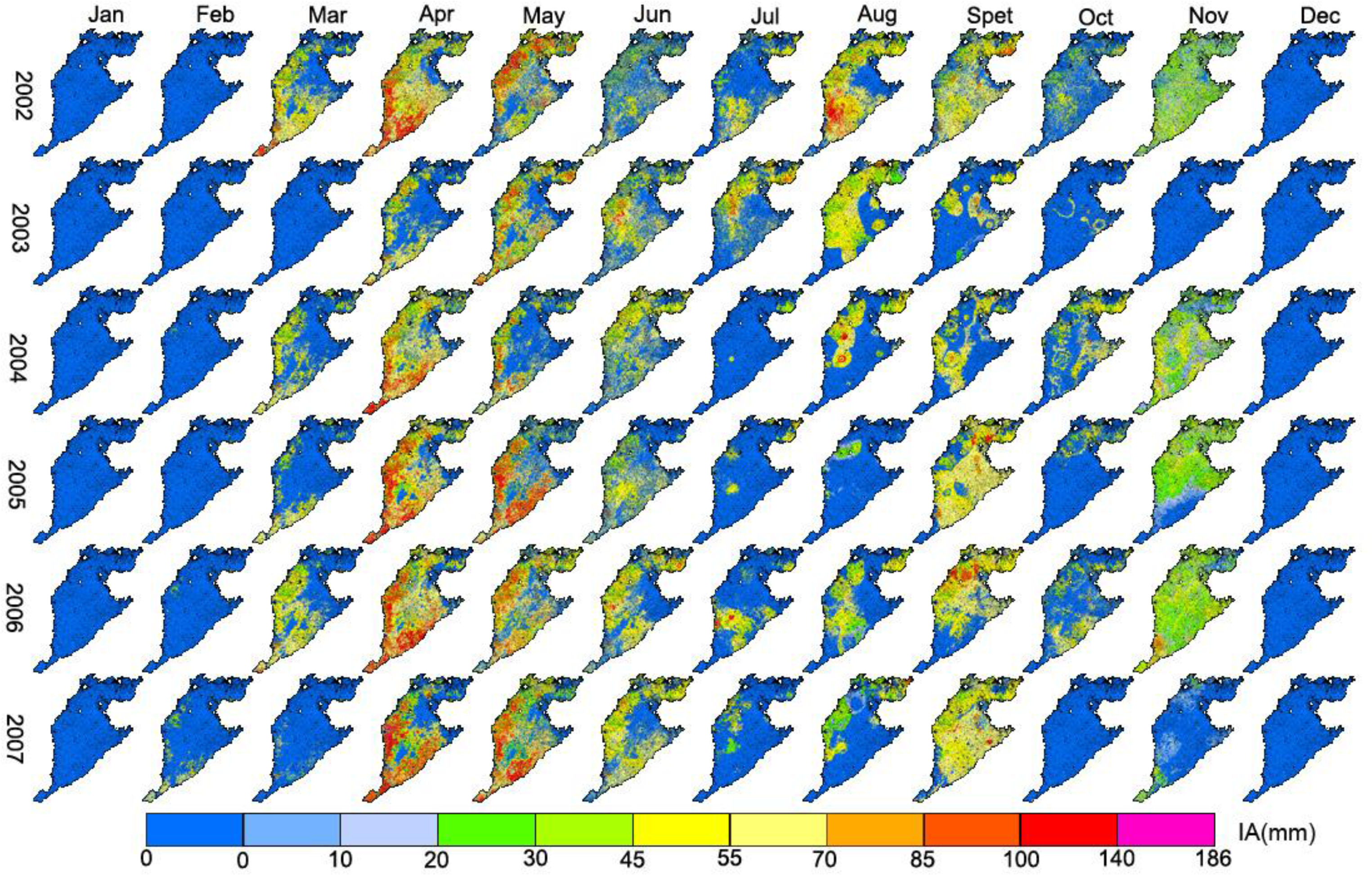
5.3. Monthly Spatial Distribution of ET and IA
5.4. Reallocation of Water Resources after SNWT Project in Hebei Plain
6. Discussion
6.1. Comparison with Contemporary Studies
6.2. Bias Analysis
6.3. Suggestion for the Sustainability of Water Resources
7. Conclusions
Acknowledgments
Author Contributions
Conflicts of Interest
Reference
- Ahmad, M.D.; Turral, H.; Nazeer, A. Diagnosing irrigation performance and water productivity through satellite remote sensing and secondary data in a large irrigation system of Pakistan. Agric. Water Manag 2009, 96, 551–564. [Google Scholar]
- Wriedt, G.; van der Velde, M.; Aloe, A.; Bouraoui, F. Estimating irrigation water requirements in Europe. J. Hydrol 2009, 373, 527–544. [Google Scholar]
- Boken, V.K.; Hoogenboom, G.; Hook, J.E.; Thomas, D.L.; Guerra, L.C.; Harrison, K.A. Agricultural water use estimation using geospatial modeling and a geographic information system. Agric. Water Manag 2004, 67, 185–199. [Google Scholar]
- Allen, R.G. Using the FAO-56 dual crop coefficient method over an irrigated region as part of an evapotranspiration intercomparison study. J. Hydrol 2000, 229, 27–41. [Google Scholar]
- Knox, J.W.; Weatherhead, K.; Loris, A.A.R. Assessing water requirements for irrigated agriculture in Scotland. Water Int 2007, 32, 133–144. [Google Scholar]
- Ozdogan, M.; Woodcock, C.E.; Salvucci, G.D.; Demir, H. Changes in summer irrigated crop area and water use in Southeastern Turkey from 1993 to 2002: Implications for current and future water resources. Water Resour. Manag 2006, 20, 467–488. [Google Scholar]
- Leenhardt, D.; Trouvat, J.L.; Gonzales, G.; Perarnaud, V.; Prats, S.; Bergez, J.E. Estimating irrigation demand for water management on a regional scale II. Validation of ADEAUMIS. Agric. Water Manag 2004, 68, 233–250. [Google Scholar]
- Ines, A.V.M.; Das Gupta, A.; Loof, R. Application of GIS and crop growth models in estimating water productivity. Agric. Water Manag 2002, 54, 205–225. [Google Scholar]
- Guerra, L.C.; Garcia y Garcia, A.; Hook, J.E.; Harrison, K.A.; Thomas, D.L.; Stooksbury, D.E.; Hoogenboom, G. Irrigation water use estimates based on crop simulation models and kriging. Agric. Water Manag 2007, 89, 199–207. [Google Scholar]
- Liu, J.G.; Williams, J.R.; Zehnder, A.J.B.; Yang, H. GEPIC—Modelling wheat yield and crop water productivity with high resolution on a global scale. Agric. Syst 2007, 94, 478–493. [Google Scholar]
- Hadria, R.; Duchemin, B.; Baup, F.; Le Toan, T.; Bouvet, A.; Dedieu, G.; Le Page, M. Combined use of optical and radar satellite data for the detection of tillage and irrigation operations: Case study in Central Morocco. Agric. Water Manag 2009, 96, 1120–1127. [Google Scholar] [Green Version]
- Ines, A.V.M.; Honda, K.; Das Gupta, A.; Droogers, P.; Clemente, R.S. Combining remote sensing-simulation modeling and genetic algorithm optimization to explore water management options in irrigated agriculture. Agric. Water Manag 2006, 83, 221–232. [Google Scholar]
- Bastiaanssen, W.G.M.; Noordman, E.J.M.; Pelgrum, H.; Davids, G.; Thoreson, B.P.; Allen, R.G. SEBAL model with remotely sensed data to improve water-resources management under actual field conditions. J. Irrig. Drain. Eng. Asce 2005, 131, 85–93. [Google Scholar]
- Wu, B.; Xiong, J.; Yan, N.; Yang, L.; Du, X. ETWatch for monitoring regional evapotranspiration with remote sensing. Adv. Water Sci 2008, 19, 671–678. [Google Scholar]
- Yang, G.Y.; Wang, Z.S.; Wagn, H.; Jia, Y.W. Potential evapotranspiration evolution rule and its sensitivity analysis in Haihe River Basin. Adv. Water Sci 2009, 20, 409–415. [Google Scholar]
- Zheng, S.; Li, X. Study on water resources and its sustainable use in the Haihe River Basin. South North Water Trans. Water Sci. Tech 2009, 7, 45–77. [Google Scholar]
- Liu, C.M. Environmental issues and the south-north water transfer scheme. China Q 1998, 899–910. [Google Scholar]
- Wu, B.; Yan, N.; Xiong, J.; Bastiaanssen, W.G.M.; Zhu, W.; Stein, A. Validation of ETWatch using field measurements at diverse landscapes: A case study in Hai Basin of China. J. Hydrol 2012, 436, 67–80. [Google Scholar]
- Wu, B.X.; Xiong, J.; Yan, N.; Yang, L. ETWatch: An Operational ET Monitoring System with Remote Sensing. Proceedings of the 2008 ISPRS Workshop on Geo-information and Decision Support Systems, Tehran, Iran, 6–7 January 2008.
- Sun, H.; Shen, Y.; Yu, Q.; Flerchinger, G.N.; Zhang, Y.; Liu, C.; Zhang, X. Effect of precipitation change on water balance and WUE of the winter wheat-summer maize rotation in the North China Plain. Agric. Water Manag 2010, 97, 1139–1145. [Google Scholar]
- Saxton, K.; Rawls, W. Soil water characteristic estimates by texture and organic matter for hydrologic solutions. Soil Sci. Soc. Am. J 2006, 70, 1569–1578. [Google Scholar]
- LAADS Web: Level 1 and Atmosphere Archive and Distribution System. Available online: http://ladsweb.nascom.nasa.gov/data/search.html (accessed 3 March 2013).
- Kaufman, Y.J.W.; Remer, L.A.; Gao, B.; Li, R.; Flynn, L. The MODIS 21 μm channel—Correlation with visible reflectance for use in remote sensing of aerosol. IEEE Trans. Geosci. Remote Sens 1997, 35, 1–13. [Google Scholar]
- Vermote, E.F.; Tanre, D.; Deuze, J.L.; Herman, M.; Morcrette, J.J. Second simulation of the satellite signal in the solar spectrum, 6S: An overview. IEEE Trans. Geosci. Remote Sens 1997, 35, 675–686. [Google Scholar]
- Mao, K.; Qin, Z.; Shi, J.; Gong, P. A practical split-window algorithm for retrieving land-surface temperature from MODIS data. Int. J. Remote Sens 2005, 26, 3181–3204. [Google Scholar]
- Xiong, J.; Wu, B.; Yan, N.; Zeng, Y.; Liu, S. Estimation and validation of land surface evaporation using remote sensing and meteorological data in North China. IEEE J. Sel. Top. Appl. Earth Obs. Remote Sens 2010, 3, 337–344. [Google Scholar]
- Legates, D.R.; McCabe, G.J. Evaluating the use of “goodness-of-fit” measures in hydrologic and hydroclimatic model validation. Water Resour. Res 1999, 35, 233–241. [Google Scholar]
- Han, S.; Yang, Y.; Lei, Y.; Tang, C.; Moiwo, J.P. Seasonal groundwater storage anomaly and vadose zone soil moisture as indicators of precipitation recharge in the piedmont region of Taihang Mountain, North China Plain. Hydrol. Res 2008, 39, 479–495. [Google Scholar]
- Water Resources Department of Hebei Province. Yearbook of Hebei Province Water Resources Statistic 1986–2006; Hebei Province Statistical Publishing House: Shijiazhuang, China, 2007; In Chinese. [Google Scholar]
- Li, Y.D. Controlling ET to ensure the sustainable exploitation of water resources in Haihe Catchment. Hydrol. Haihe Catch 2007, 1, 4–8. [Google Scholar]
- Yu, W.D. Water balance and water resources sustainable development in Haihe River Basin. J. China Hydrol 2008, 28, 79–82. [Google Scholar]
- Yang, Y.; Yang, Y.; Moiwo, J.P.; Hu, Y. Estimation of irrigation requirement for sustainable water resources reallocation in North China. Agric. Water Manag 2010, 97, 1711–1721. [Google Scholar]
- Yang, Y.; Watanabe, M.; Zhang, X.; Hao, X.; Zhang, J. Estimation of groundwater use by crop production simulated by DSSAT-wheat and DSSAT-maize models in the piedmont region of the North China Plain. Hydrol. Process 2006, 20, 2787–2802. [Google Scholar]
- Water Resources Department of Hebei Province. Report on Exploitation Planning for Hebei Provincial Groundwater Resources; Hebei Province Statistical Publishing House: Shijiazhuang, China, 1998; In Chinese. [Google Scholar]
- Hu, Y.; Moiwo, J.P.; Yang, Y.; Han, S.; Yang, Y. Agricultural water-saving and sustainable groundwater management in Shijiazhuang Irrigation District, North China Plain. J. Hydrol 2010, 393, 219–232. [Google Scholar]


| 2005 | 2006 | 2007 | ||||
|---|---|---|---|---|---|---|
| Observed | Modelled | Observed | Modelled | Observed | Modelled | |
| Mean, mm | 240 | 224 | 295 | 299 | 246 | 202 |
| Standard deviation, mm | 74 | 50 | 91 | 72 | 95 | 80 |
| Mean absolute error, mm | 38.88 | 39.75 | 52.05 | |||
| Root mean square error, mm | 53 | 55 | 71 | |||
| Pearson’s correlation | 0.73 | 0.80 | 0.81 | |||
| Coefficient of determination | 0.53 | 0.64 | 0.65 | |||
| Modified index of agreement | 0.61 | 0.68 | 0.68 | |||
© 2014 by the authors; licensee MDPI, Basel, Switzerland This article is an open access article distributed under the terms and conditions of the Creative Commons Attribution license (http://creativecommons.org/licenses/by/3.0/).
Share and Cite
Yang, Y.; Yang, Y.; Liu, D.; Nordblom, T.; Wu, B.; Yan, N. Regional Water Balance Based on Remotely Sensed Evapotranspiration and Irrigation: An Assessment of the Haihe Plain, China. Remote Sens. 2014, 6, 2514-2533. https://doi.org/10.3390/rs6032514
Yang Y, Yang Y, Liu D, Nordblom T, Wu B, Yan N. Regional Water Balance Based on Remotely Sensed Evapotranspiration and Irrigation: An Assessment of the Haihe Plain, China. Remote Sensing. 2014; 6(3):2514-2533. https://doi.org/10.3390/rs6032514
Chicago/Turabian StyleYang, Yanmin, Yonghui Yang, Deli Liu, Tom Nordblom, Bingfang Wu, and Nana Yan. 2014. "Regional Water Balance Based on Remotely Sensed Evapotranspiration and Irrigation: An Assessment of the Haihe Plain, China" Remote Sensing 6, no. 3: 2514-2533. https://doi.org/10.3390/rs6032514